The influence of gait speed on local dynamic stability of walking

Abstract

The focus of this study was to examine the role of walking velocity in stability during normal gait. Local dynamic stability was quantified through the use of maximum finite-time Lyapunov exponents, λ_Max. These quantify the rate of attenuation of kinematic variability of joint angle data recorded as subjects walked on a motorized treadmill at 20%, 40%, 60%, and 80% of the Froude velocity. A monotonic trend between λ_Max and walking velocity was observed with smaller λ_Max at slower walking velocities. Smaller λ_Max indicates more stable walking dynamics. This trend was evident whether stride duration variability remained or was removed by time normalizing the data. This suggests that slower walking velocities lead to increases in stability. These results may reveal more detailed information on the behavior of the neuro-controller than variability-based analyses alone.

1. Introduction

Stability is a critical component of walking [10,14]. It can be defined as the ability to maintain functional locomotion despite the presence of small kinematic disturbances or control errors. Stability of standing static postures is often recorded from kinematic variability associated with the center-of-pressure under the equilibrium base of support. However, walking is a dynamic condition wherein the joint control torques change with time and posture. Therefore, stability of walking requires analyses that account for both time and movement [16]. Kinematics of walking and associated variability are influenced by walking velocity thereby indicating potential velocity effects on stability [17,19]. Some studies suggest that one possible motivation for slower walking speed in the elderly and in individuals with joint disease and neuropathology is to improve stability [6]. This assumes that stability of walking is improved at slower velocities. The purpose of this study was to test this assumption.

There is a difference between kinematic variability and stability. Studies have measured the magnitude of kinematic variability as an estimate of stability [11,25]. It is often assumed that increased variability corresponds to decreased stability. However, measurements of kinematic variability are subtly different than stability. It is reasonable to assume that every walking stride could be similar to every other stride. Natural kinematic variance observed in empirical data is therefore attributed to mechanical disturbances or control errors. These disturbances are attenuated in time by the neuro-controller and musculoskeletal system in order to maintain a stable walking pattern. Thus, stability must be estimated from the time-dependent expansion or attenuation of kinematic variability [10,14].

Stability of human walking can be estimated from temporal analyses of multi-dimensional variability [4]. Disturbance to the walking trajectory is an ongoing process so the attenuation of kinematic variability is continually manifest. Poincare maps quantify the attenuation of kinematic variability between consecutive strides [14]. This method has the advantage of measuring stability in a multi-degree-of-freedom system. However, it provides limited insight regarding intra-stride effects and often ignores expansion in temporal variability, e.g. stride-duration variance. Effects from a kinematic disturbance can be observed over a time scale that influences both intra-stride and inter-stride movement [11]. Dynamic analyses can be used to track the time-history of individual disturbances recorded from the time-dependent kinematics [16]. The time-dependent rate of kinematic expansion is measured by the Lyapunov exponent, λ. One Lyapunov exponent exists for every movement dimension of the analyzed kinematic trajectory. These can be arranged, in order of most rapidly diverging to most rapidly converging, as λ₁ > λ₂ > > λ_n. To avoid confusion, λ₁ may be referred to as λ_Max to represent the largest Lyapunov exponent. Rosenstein et al. concluded that when using the full Lyapunov spectrum, a system is stable when the sum of these Lyapunov exponents is negative, i.e. the rate of convergence is greater than the rate of divergence [22]. Calculation of the full Lyapunov spectrum from experimental data, however, is exceedingly difficult. These calculations may be simplified greatly by realizing that two randomly selected initial trajectories should diverge, on average, at a rate determined by the largest Lyapunov exponent, λ_Max. Calculation of λ_Max is relatively easy and can be used to evaluate the influence of walking velocity on dynamic stability of walking.

The goal of this study was to (1) implement Lyapunov analyses to characterize stability of dynamic steady-state walking, and (2) test whether walking velocity influences stability of walking. This is the first in a series of studies planned to quantify the stability of gait in normal-developing subjects and patients with developmental neuro-impairment.

2. Methods

2.1. Experimental procedures

Kinematic data were recorded from 19 healthy adult subjects including 6 males and 13 females; mean age (±S.D.) 22.5 ± 2.8 years; mean height 1.7 ± 0.1 m and mean weight 65.7 ± 12.7 kg. Lower-body kinematic data were recorded from 21 reflective markers using a 6-camera, 3D, video motion analysis system at a data sampling rate of 240 Hz (Vicon, Oxford Metrics). Markers were placed on the sacrum, anterior superior iliac spine, posterior superior iliac spine, anterior thigh, lateral epicondyle of the femur, anterior shin, lateral malleolus of the fibula, dorsum of the foot, 5th metatarsal, calcaneous and hallux. Subjects walked barefoot on a treadmill at 20%, 40%, 60% and 80% of their Froude velocity, V_F. Walking velocity was expressed in terms of Froude velocity to appropriately scale the walking speed to leg length and pendulum dynamics [24]. Each subject's Froude velocity (square root of Froude number) was calculated based on the equation:

$$V_{\mathrm{F}}=\sqrt[]{\mathit{Rg}}$$ (1)

where R is the distance between the greater trochanter and lateral malleolus of the fibula and g is the acceleration due to gravity. Comfortable walking speed is typically 0.42 V_F and running is initiated at 0.70 V_F [2,15]. Therefore, stability was recorded at walking velocities near the comfortable walking speed, slow walking, fast walking, and at speeds in excess of the natural walk-run transition.

Four repeated collections of 30 walking strides per velocity condition were recorded for each subject. Ankle, knee and hip angles were calculated from the 3D locations of the marker set using standard techniques (MATLAB, Mathworks, Inc., Natick, MA). Analyses were limited to the plantarflexion/dorsiflexion dimension of the ankle, knee flexion angle and hip flexion angle. Previous studies recommend against filtering the data before Lyapunov analyses so as to retain spatio-temporal fluctuations and nonlinearities [8]. However, we believe that kinematic signals at frequencies greater than 10 Hz are unlikely related to the musculoskeletal motion and therefore filtered the data with a 10 Hz, low-pass second-order Butterworth filter. Regardless of this difference in opinion regarding filtering the results were similar between these studies.

Since cadence changes with walking velocity but data sampling frequency remained fixed, a dilemma arises with respect to the proper way to compare data collected at different walking velocities. Specifically, since stride-duration decreases with walking velocity, data collected at 80% V_F would likely have less than half as many data points per stride, on average, as data collected at 20% V_F. Data were time-normalized in two separate manners and results compared. First, every stride was time-normalized to 100 data points per stride. This provides an equal number of data points per stride regardless of velocity but it removes stride-to-stride temporal variations that are an important component of Lyapunov stability analyses. Second, data sets of 30 contiguous strides were re-sampled to be 3000 data points long, i.e. approximately 100 data points per stride on average but any individual stride could be greater than or less than 100 data points. This permits stride-to-stride temporal variation while normalizing the data such that the average number of data points per stride were similar for each velocity condition. In an attempt to understand the influence of re-sampling frequency on the Lyapunov analysis, the same data were also analyzed with data re-sampled to 1500 data points. Independent stability analyses were performed on each time-dependent joint angle, x_j(t), where j = 1:6 was the joint number and t was the re-sampled time interval.

2.2. Calculating dynamic stability

Local dynamic stability was determined based on the maximum finite-time Lyapunov exponent, λ_Max. These were used to quantify the exponential attenuation of variability between neighboring kinematic trajectories. The approach assumes that every stride could be identical to every other stride. Stride-to-stride differences in kinematic measurements are attributed to small perturbations. Therefore, kinematic variability can be used to evaluate the stability of the system by tracking the progression of a perturbed gait cycle back to the mean. Since the recorded time-series data, x_j(t), are one dimensional column vectors of joint angles it was necessary to reconstruct an n-dimensional state-space out of the kinematic data in order to accurately determine dynamic perturbations to the ideal gait cycle. One typical method of creating an n-dimensional state-space from scalar data is by method of delays. Using this method a joint angle in n-dimensional space would appear as

$$Y_j\left(t\right)=[x_j\left(t\right),x_j(t+T_{\mathrm{d}}),x_j(t+2T_{\mathrm{d}})\cdots x_j(t+(n-1)T_{\mathrm{d}})]$$ (2)

where x_j(t) is the original scalar data of joint angle and T_d is a constant time delay. A reconstructed state-space Y_j(t) with an embedding dimension of n = 3 can be seen in Fig. 1A.

Fig. 1.

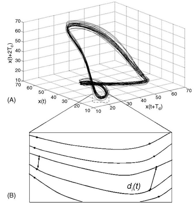
(A) Reconstructed state-space kinematics of knee angle with three embedded dimensions. Fifteen contiguous strides are illustrated. (B) Divergence of nearest neighbors with temporal variability permitted.

The success of state-space reconstruction by the method of delays is sensitive to the time delay, T_d [23]. Several methods exist for calculation of T_d. There is no consensus on which method provides optimal results. Three methods have been popularized including: (1) time delays estimated from the average mutual information function [6,9], (2) time delays estimated from the time it takes for the autocorrelation function to drop to a pre-specified fraction of its initial value [20], and (3) time delays estimated using geometric approaches based on maximizing some component of the reconstructed state-space [3,23]. Using the average mutual information function and the autocorrelation approach, we observed time-delay estimates ranging from 9 to 40 samples. To assure that all of the trials were analyzed similarly, a constant T_d of 10 samples (10% of the length of the gait cycle) was used for all reconstructed state-space.

The number of state-space dimensions, n in Eq. (1), is selected based on a global false-nearest-neighbor analysis [22]. This method incrementally increases n until the number of false-nearest-neighbors approaches zero. False nearest neighbors are defined as sets of points that are very close to each other at dimension n = k but not at n = k + 1. For example, a plot of x(t) = sin(2π^t) + cos(πt) with n = 3 embedding dimensions in Fig. 2A illustrates that the curve does not intersect itself. When this same data is viewed in two-dimensions, n = 2, it artificially appears to cross-over itself, i.e. a false nearest neighbor would occur at the crossover point as in Fig. 2B. A global false-nearest-neighbor analysis suggested that an embedding dimension of n = 5 was appropriate for the analyzed data.

Fig. 2.

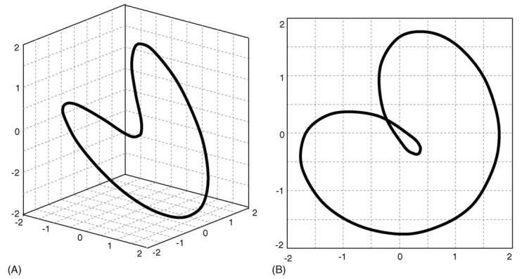
Plot of x(t) = sin(2πt) + cos(πt) with embedding dimension n = 3 (A) and n = 2 (B). Note the false-nearest-neighbor illustrated by the intersection at [−0.25, 0.25] when n =2.

Maximum finite-time Lyapunov exponents were calculated based on the algorithm published by Rosenstein et al. [22]. The Euclidean distance between nearest neighbors, dⁱ(t), was computed for each data-point, i, in the reconstructed state-space Y^j(t) for all time, t. Nearest neighbors are found by selecting data points from separate cycles that are closest to each other in reconstructed state-space as in Fig. 1B. If repeated strides were kinematically identical, then a plot of the trajectories would illustrate each cycle on top of the others in state-space. In this condition, the distance between nearest neighbors, dⁱ(t), would be zero for all pairs of nearest neighbors, i. However, in the empirically measured data the distance between nearest neighbors, dⁱ(t), was greater than zero as in Fig. 1A. Hence, there are clearly kinematic disturbances observable in the data. The distance between all nearest neighbors was tracked forward in time to record time-dependent changes in kinematic variability as in Fig. 1B. The rate of change in the distance between nearest neighbors is quantified by the Lyapunov exponents, λ:

$$d\left(t\right)=D_0{\mathrm{e}}^{\lambda t}$$ (3)

where D⁰ is the average displacement between trajectories at t = 0. Two randomly selected initial trajectories should diverge, on average, at a rate determined by the largest Lyapunov exponent, λ^Max [22]. Therefore, the maximum Lyapunov exponent, λ^Max was approximated from the experimental joint-angle data as the slope of the linear best-fit line to the curve created by the equation:

$$\langle \ln \{d_i(k+\Delta t)∕d_i\left(k\right)\}{\rangle }_i={\lambda }_{\mathrm{Max}}\Delta t$$ (4)

where 〈ln dⁱ(k)〉 represents the average logarithm of displacement for all pairs of nearest neighbors, i. The maximum finite-time Lyapunov exponent, λ^Max, was calculated as the slope of the logarithm of the average divergence across the span of 0–1 strides as shown in Fig. 3. A value of λ^Max was computed for each joint of every subject at each walking velocity. λ^Max was interpreted as a measure of dynamic stability.

Fig. 3.

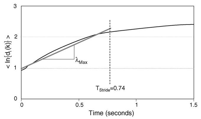
Average logarithmic divergence vs. time. The best fit linear slope of the logarithmic relation from 0 to 1 stride represents λ^Max. In this example the stride duration was 0.74 s.

Statistical analyses were performed to determine the effects of walking velocity on stability. Lyapunov exponents were computed independently for the ankle, knee and hip for each subject and each walking velocity, V^F = 20%, 40%, 60%, 80%. Preliminary analyses revealed no statistically significant differences in stability between the right and left limbs. Therefore, data from the right and left limbs were pooled for statistical analyses. Two-factor repeated measures analysis of variance (ANOVA) tested the within-subject effects of joint and walking velocity on λ^Max. Analyses were performed using commercial software (Statistica, 4.5 Statsoft, Inc., Tulsa, OK) using a significance level of α < 0.05.

3. Results

When the full 30 stride data sets at each velocity were resampled to be 3000 data points in duration, variability in stride-duration was observed despite walking at constant velocity. Mean and standard deviations of stride time were 1.57 ± 0.06 s at 20% V^F, and 1.12 ± 0.02, 0.94 ± 0.01, and 0.79 ± 0.02 s for 40%, 60%, and 80% V_F, respectively. This stride-time was significantly longer (p < 0.001) at 20% V^F than at 40%, 60%, and 80% V^F.

Maximum finite-time Lyapunov exponents, λ^Max, were calculated for each subject and velocity condition to estimate dynamic stability of walking. There was a significant main effect of joint on the stability value (p < 0.001) illustrated in Fig. 4. Mean value of λ^Max was 1.08 ± 0.35 mm/s for the ankle, 1.40 ± 0.37 mm/s for the knee, and 1.27 ± 0.34 mm/s for the hip. Post hoc analyses demonstrated that λ^Max for the ankle was significantly (p < 0.001) less than in the hip and knee. λ^Max for the hip was in turn significantly (p < 0.01) less than in the knee. Recall that smaller values of λ^Max suggest greater stability thereby indicating greater neuromuscular stabilizing control in the ankle joint than measured in the hip and knee.

Fig. 4.

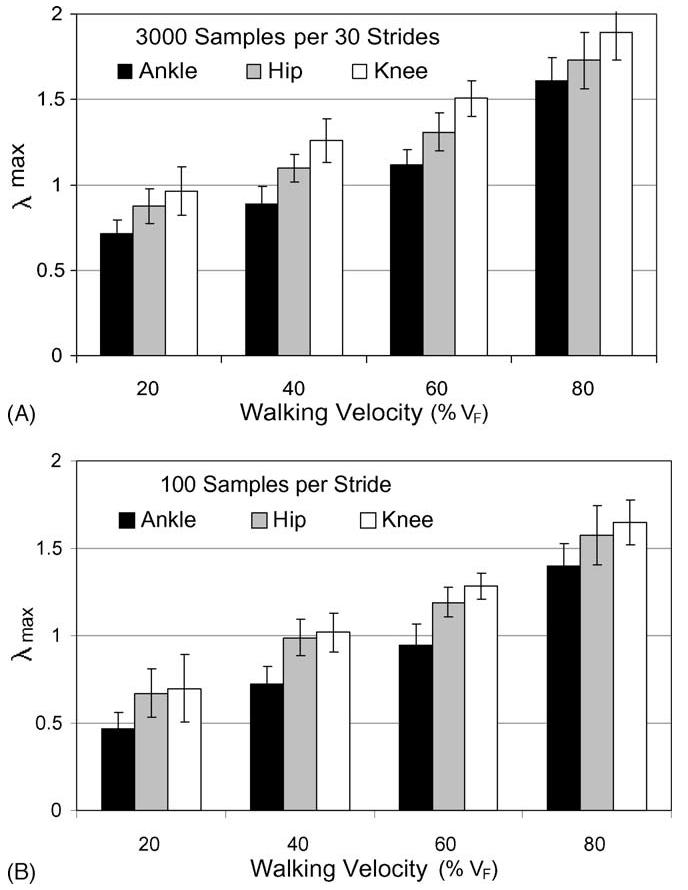
Average λ^Max increased with walking velocity. This trend was observed when data were re-sampled to 3000 samples per 30 strides (A) and similarly when temporal variability was removed by re-sampling the data to 100 samples per stride (B).

Stability was significantly (p < 0.001) influenced by the main effect of walking velocity. This effect was similarly observed whether stride-duration variability was maintained by time-normalizing at 3000 points per 30 strides, or whether stride-duration variability was eliminated by time-normalizing to exactly 100 points per stride. λ^Max at each velocity was significantly different than at every other velocity and monotonically increased with increasing velocity. Regression analyses were performed to analyze for trends related to velocity. A best-fit trendline with linear and quadratic terms was developed for each set of data for comparison with similar methods by others [8]. Results suggest the λ^Max values for the ankle were quadratically related to walking velocity, but the stability of the knee dynamics were significantly correlated with a linear behavior of walking velocity as in Table 1. Data re-sampled to 3000 data points per 30 strides were compared to data re-sampled to 1500 data points per 30. Halving the effective sampling frequency caused a significantly (p < 0.001) reduced λ^Max.

Table 1.

Regression analysis results comparing λ_Max with walking velocity

Data Samples	Joint	Regression Equation	R2	Linear	Quadratic
100 samples per stride	Ankle	λMax = 12.2−5 x2 + 2.9−3 x + 0.372	0.898	p = 0.397	p = 0.001
,	Knee	λMax = 3.1−5 x2 + 1.2−3 x + 0.444	0.876	p = 0.002	p = 0.418
	Hip	λMax = 4.1−5 x2 + 10.5−3 x + 0.460	0.864	p = 0.008	p = 0.287
3000 samples per 30 strides	Ankle	λMax = 19.8−5 x2 − 5.2−3 x + 0.748	0.912	p = 0.089	p = 0.001
	Knee	λMax = 5.7−5 x2 + 9.5−3 x + 0.759	0.868	p = 0.015	p = 0.136
	Hip	λMax = 9.5−5 x2 + 4.5−3 x + 0.755	0.852	p = 0.240	p = 0.013

Two of the three measurements were linearly related to velocity when stride-duration variability was removed (100 samples per stride). Two of the three measurements were related in a quadratic manner to walking velocity when stride-duration variability was retained (3000 samples per 30 strides).

4. Discussion

It has been suggested that individuals with impaired neuromuscular control may walk with reduced velocity in order to improve their stability [5]. Existing evidence reveals that kinematic and spatio-temporal variability are influenced by walking velocity [19]. However, stability might be poorly represented by the magnitude of variability. Instead, assessment of stability requires examination of how the neuro-control system handles kinematic variability, i.e. the active and passive control of disturbances. Therefore, the goal of the current study was to determine the relationship between walking velocity and the Lyapunov exponent that represents the time-dependent change in joint angle variability. Dingwell and Marin [8] recently reported results from a similar study to investigate the influence of walking velocity on stability. They observed that kinematic variability demonstrated a quadratic behavior, i.e. variability was least near the comfortable walking velocity but it was increased at both slow and fast walking velocities. Conversely, their analyses suggest that stability increased linearly with walking velocity. Our analyses agree with this monotonic trend.

Lyapunov analyses revealed that stability was significantly influenced by walking velocity. When the data from every stride were time-normalized to 100 data points per stride, a linear relationship was observed between λ^Max and velocity. Smaller λ^Max represents a more stable system. Therefore, every joint was significantly more stable at lower velocities. These results agree with the conclusions of Dingwell and Marin [8] despite differences in measurement techniques and processing. However, this method of time-normalizing the data artificially removes stride-to-stride temporal variations. A kinematic disturbance can influence not only the movement pattern but it can also influence the time duration of the movement trajectory. To accommodate stride-duration variability separate analyses were performed wherein the data from 30 strides were time-normalized to 3000 data points in total. This process causes a mean stride-duration of 100 points per cycle but all strides were not necessarily of equal length. In fact, results demonstrate mean stride-to-stride variation of 2.3%. Using this time-normalizing procedure walking velocity continued to significantly influence the Lyapunov exponent, λ^Max, i.e. monotonic trend of lower stability at faster walking velocities. Unlike the analyses with exactly 100 points per stride, the temporal variation introduces a more quadratic trend.

Fast walking velocity may influence dynamic stability by a combination of several mechanisms. Walking velocity affects kinematics, double-support time, step width and other clinical correlates of stable walking [1]. Modified support mechanics may influence the ability to control movement disturbances. Analyses of bipedal walking demonstrate the existence of a biomechanical resonance associated the pendulum-like behavior of the skeletal structure and muscle stiffness [12]. These may contribute to stability at the preferred walking velocity [18]. Therefore, walking at velocities that are faster or slower than this resonant frequency require greater active neuromuscular control to maintain stable periodic movement [21]. In other words, faster walking velocities increase the segmental momentum thereby requiring greater effort from the neuro-controller to attenuate kinematic disturbances. Short stride durations limit the allowable time for neuromuscular corrections to compensate for mechanical disturbances or controller errors. The slow walking velocity requires active control that is out-of-phase with movement in order to slow the natural dynamics of the passive system. Hence, most of the variability observed by the Lyapunov exponents during the slow walking velocity appeared to be attributable to fluctuations in stride duration whereas during fast walking the variability was primarily associated with kinematic disturbances. This suggests that these subjects may be temporally less stable at the slow walking velocity than at fast walking velocities but spatially more stable at the slow velocity. Nonetheless, results suggest that the neuro-control system more effectively controlled kinematic disturbances at the slow velocity than during fast walking.

Data processing and analyses techniques must be considered when interpreting the results. Rosenstein et al. [22] observed that Lyapunov analyses are sensitive to the sampling frequency and length of the data set. If the sampling frequency is sufficient to characterize the kinematic variance then the length of the data set is more critical than sampling frequency. If one were to use a common sampling rate for all velocities, then the length of the data set at 80% V^F would include approximately half the number of data samples per stride when compared to 20% V^F. The only other study that directly compared walking velocity to dynamic stability compared 3 min of gait data collected between 60% and 140% of a subject's preferred walking speed [8]. This would indicate walking velocities of approximately 27%, 45%, and 63% V^F that were similar to the walking speeds in the current study. In their study, a fast trial may potentially have more than twice as many strides with half as many data points per stride compared to a slow walking trial, i.e. greater sample density at slow velocities than at fast velocities. To investigate the effect of halving the number of data samples per stride, we compared results from data that were re-sampled at 3000 samples per 30 strides versus results from the same walking trials that were re-sampling at 1500 samples per 30 strides. Note that both re-sample rates retained the stride-to-stride temporal variation of the original kinematic data. Shorter data set lengths reduced the mean value of λ^Max by 17.2%. Thus, when comparing the stability of different walking velocities it is necessary to account for the effects of data sampling rate and differences in data set lengths. To avoid artifacts from sample density we recommend that stability analyses should normalized the time scale so that there are an approximately equivalent number data points at fast walking velocity as at slow velocity.

Several experimental and analytical limitations should be addressed in future research. First, the maximum finite-time Lyapunov exponent, λ^Max, represents the greatest rate of divergence in the kinematic data but there are other dimensions wherein errors are attenuated at a rate represented by the remaining λ coefficients. To fully characterize the stability of the walking process the full set of Lyapunov exponents should be investigated. Second, in a previous study of walking dynamics the stability of walking was determined from a sensor placed over the first thoracic vertebrae [8]. Those measurements represent the instantaneous kinematic expansion from the coupled dynamics of individual segment movement from the lower limbs. However, we observed significant stability differences in individual joints thereby indicating that the risk of failure may be related to specific joints. Further analyses require matrix formulation wherein separate Lyapunov coefficients are determined for homologous and multi-joint interactions to characterize dynamic stability of locomotion. Third, the results may be influenced by the fact that data were collected while subjects walked on treadmill. Due to the spatial constraints of the video motion capture system; a treadmill was necessary to enable collection of kinematic data across many sequential strides. Studies have shown that a treadmill may reduce kinematic variability and increase dynamic stability of gait measures [7]. Finally, our results were limited to healthy adults. The influence of neuromuscular impairment may modify not only the stability of walking [13] but the relation between walking velocity and stability.

In conclusion, dynamic stability of walking is influenced by walking velocity with different contributions from the ankle, knee and hip joints. Analyses of clinical outcomes often demonstrate improved walking velocity following interventions indicating possible improvements in stability [1]. We recommend that clinical assessments should be expanded where possible to investigate whether (1) patients with neuromuscular impairment have abnormal stability and (2) whether conventional treatments successfully improve the stability of walking performance. These dynamic stability analyses may provide improved insight into neuromuscular control of dynamic locomotion.

Appendix A. Supplementary data

Supplementary data associated with this article can be found, in the online version, at doi:10.1016/j.gaitpost. 2006.03.003.

References

- 1.Abel MF, Damiano DL. Strategies for increased walking speed in diplegic cerebral palsy. J Ped Orthop. 1996;16:753–8. doi: 10.1097/00004694-199611000-00010. [DOI] [PubMed] [Google Scholar]
- 2.Ahlborn BK, Blake RW. Walking and running at resonance. Zoology (Jena) 2002;105:165–74. doi: 10.1078/0944-2006-00057. [DOI] [PubMed] [Google Scholar]
- 3.Buzug T, Pfister G. Optimal delay time and embedding dimension for delay-time coordinates by analysis of the global static and local dynamic behavior of strange attractors. Phys Rev A. 1992;45:7073–84. doi: 10.1103/physreva.45.7073. [DOI] [PubMed] [Google Scholar]
- 4.Buzzi UH, Stergiou N, Kurz MJ, Hageman PA, Heidel J. Nonlinear dynamics indicates aging affects variability during gait. Clin Biomech (Bristol Avon) 2003;18:435–43. doi: 10.1016/s0268-0033(03)00029-9. [DOI] [PubMed] [Google Scholar]
- 5.Dingwell JB, Cavanagh PR. Increased variability of continuous over-ground walking in neuropathic patients is only indirectly related to sensory loss. Gait Posture. 2001;14:1–10. doi: 10.1016/s0966-6362(01)00101-1. [DOI] [PubMed] [Google Scholar]
- 6.Dingwell JB, Cusumano JP. Nonlinear time series analysis of normal and pathological human walking. Chaos. 2000;10:848–63. doi: 10.1063/1.1324008. [DOI] [PubMed] [Google Scholar]
- 7.Dingwell JB, Cusumano JP, Cavanagh PR, Sternad D. Local dynamic stability versus kinematic variability of continuous overground and treadmill walking. J Biomech Eng Transact ASME. 2001;123:27–32. doi: 10.1115/1.1336798. [DOI] [PubMed] [Google Scholar]
- 8.Dingwell JB, Marin LC. Kinematic variability and local dynamic stability of upper body motions when walking at different speeds. J Biomech. 2006;39:444–52. doi: 10.1016/j.jbiomech.2004.12.014. [DOI] [PubMed] [Google Scholar]
- 9.Fraser AM, Swinney HL. Independent coordinates for strange attractors from mutual information. Phys Rev A. 1986;33:1134–40. doi: 10.1103/physreva.33.1134. [DOI] [PubMed] [Google Scholar]
- 10.Goswami A, Espiau B, Thuilot B. A study of passive gait of a compas-like biped robot: symmetry and Chaos. Int J Robot Res. 1998;17:1282–301. [Google Scholar]
- 11.Hausdorff JM, Zemany L, Peng CK, Goldberger AL. Maturation of gait dynamics: stride-to-stride variability and its temporal organization in children. J Appl Physiol. 1999;86:1040–7. doi: 10.1152/jappl.1999.86.3.1040. [DOI] [PubMed] [Google Scholar]
- 12.Holt KG, Hamill J, Andres RO. The force-driven harmonic oscillator as a model for human locomotion. Human Mov Sci. 1990;9:55–68. [Google Scholar]
- 13.Hurmuzlu Y, Basdogan C, Stoianovici D. Kinematics and dynamic stability of the locomotion of post-polio patients. J Biomech Eng. 1996;118:405–11. doi: 10.1115/1.2796024. [DOI] [PubMed] [Google Scholar]
- 14.Hurmuzlu Y, Basdogan C. On the measurement of dynamic stability of human locomotion. J Biomech Eng. 1994;116:30–6. doi: 10.1115/1.2895701. [DOI] [PubMed] [Google Scholar]
- 15.Kram R, Domingo A, Ferris DP. Effect of reduced gravity on the preferred walk-run transition speed. J Exp Biol. 1997;200:821–6. doi: 10.1242/jeb.200.4.821. [DOI] [PubMed] [Google Scholar]
- 16.Leipholz H. Stability theory. an introduction to the stability of dynamic systems and rigid bodies. John Wiley and Sons; New York: 1987. [Google Scholar]
- 17.Maki BE. Gait changes in older adults: predictors of falls or indicators of fear. J Am Geriatr Soc. 1997;45:313–20. doi: 10.1111/j.1532-5415.1997.tb00946.x. [DOI] [PubMed] [Google Scholar]
- 18.McGeer T. Passive dynamic walking. Intern J Robot Res. 1990;9:68–82. [Google Scholar]
- 19.Oberg T, Karsznia A, Oberg K. Basic gait parameters: reference data for normal subjects, 10–79 years of age. J Rehabil Res Dev. 1993;30:210–23. [PubMed] [Google Scholar]
- 20.Patla AE. Strategies for dynamic stability during adaptive human locomotion. IEEE Eng Med Biol Magaz. 2003;22:48–52. doi: 10.1109/memb.2003.1195695. [DOI] [PubMed] [Google Scholar]
- 21.Ralston HJ. Energy-speed relation to optimal speed during level walking. Int Z Angew Physiol. 1958;17:277–83. doi: 10.1007/BF00698754. [DOI] [PubMed] [Google Scholar]
- 22.Rosenstein MT, Collins JJ, Deluca CJ. A practical method for calculating largest Lyapunov exponents from small data sets. Phys D. 1993;65:117–34. [Google Scholar]
- 23.Rosenstein MT, Collins JJ, Deluca CJ. Reconstruction expansion as a geometry-based framework for choosing proper delay times. Phys D. 1994;73:82–98. [Google Scholar]
- 24.Vaughan CL, Langerak NG, O'Malley MJ. Neuromaturation of human locomotion revealed by non-dimensional scaling. Exp Brain Res. 2003;153:123–7. doi: 10.1007/s00221-003-1635-x. [DOI] [PubMed] [Google Scholar]
- 25.Winter DA. Biomechanics of normal and pathological gait: implications for understanding human locomotor control. J Mot Behav. 1989;21:337–55. doi: 10.1080/00222895.1989.10735488. [DOI] [PubMed] [Google Scholar]
Associated Data
This section collects any data citations, data availability statements, or supplementary materials included in this article.