A simple model for calculating the kinetics of protein folding from three-dimensional structures

Abstract

An elementary statistical mechanical model was used to calculate the folding rates for 22 proteins from their known three-dimensional structures. In this model, residues come into contact only after all of the intervening chain is in the native conformation. An additional simplifying assumption is that native structure grows from localized regions that then fuse to form the complete native molecule. The free energy function for this model contains just two contributions—conformational entropy of the backbone and the energy of the inter-residue contacts. The matrix of inter-residue interactions is obtained from the atomic coordinates of the three-dimensional structure. For the 18 proteins that exhibit two-state equilibrium and kinetic behavior, profiles of the free energy versus the number of native peptide bonds show two deep minima, corresponding to the native and denatured states. For four proteins known to exhibit intermediates in folding, the free energy profiles show additional deep minima. The calculated rates of folding the two-state proteins, obtained by solving a diffusion equation for motion on the free energy profiles, reproduce the experimentally determined values surprisingly well. The success of these calculations suggests that folding speed is largely determined by the distribution and strength of contacts in the native structure. We also calculated the effect of mutations on the folding kinetics of chymotrypsin inhibitor 2, the most intensively studied two-state protein, with some success.

The classical protein folding problem has been to predict the three-dimensional structure from the amino acid sequence. A second interesting problem is to use the known three-dimensional structure to predict the kinetics and mechanism of folding. This has taken on new importance with the recognition that many human diseases are caused by the aggregation of partially folded or misfolded proteins (1). Several developments over the past decade have made the theoretical prediction of folding kinetics a realistic goal. The first is the acquisition of detailed experimental data on 18 small single-domain proteins of known structure that show two-state equilibrium and kinetic behavior, which was first observed for chymotrypsin inhibitor 2 (CI2) by Jackson and Fersht (2). These studies provide the experimental results (3) necessary for testing theoretical models. Second, the energy landscape approach, beginning with the work of Bryngelson and Wolynes (4), has provided a coherent description of both real folding experiments and computer simulations of folding (5–13). A major simplifying result of this approach is the finding that diffusion on a one-dimensional free energy surface can reproduce folding rates observed in computer simulations of simplified representations of proteins (14, 15). The implication is that folding rates of real proteins could be obtained by calculating a sufficiently accurate free energy as a function of an appropriate reaction coordinate (16–18). Finally, Baker and coworkers made a key observation that folding rates of two-state proteins are correlated with topological complexity in a simple way, suggesting that a simple model could be successful (19). Such a model had already been developed (20, 21) to quantitatively explain our experiments (20) on a 16-residue, β-hairpin forming peptide. In that study, it was found that hairpin formation contains most of the basic features of protein folding, suggesting that the model might work for proteins. Here, we use the model to calculate folding kinetics of proteins by using their known three-dimensional structures and the experimentally determined equilibrium constants.

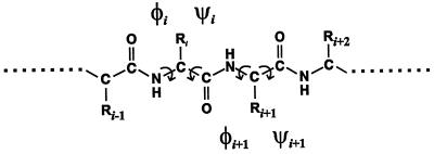
The model considers only two thermodynamic factors: stabilization by inter-residue interactions and destabilization associated with fixing backbone dihedral angles in a specific conformation (Fig. 1). Only native interactions are included; for two residues to interact, all intervening peptide bonds must be in their native conformation. The matrix of inter-residue interactions is defined by the contact map obtained from the atomic coordinates of the three-dimensional structure. The experimental free energy of protein folding is generally small [1–10 kcal/mol for the two-state proteins (3)] and results from cancellation of large enthalpic and entropic terms. It is therefore unrealistic to expect that such a simplistic thermodynamic function, with no attention to the nature of the atomic contacts, can reproduce the free energy of folding. Because we are primarily interested in the magnitude and shape of the free energy barrier separating the native and denatured states, the single parameter that describes the inter-residue interactions was adjusted for each protein so that the calculated free energy of folding agrees with the experimentally measured value. To drastically reduce the number of species in the model, only a small number of regions of native structure are permitted simultaneously in each molecule. Each of these regions is defined as a stretch of contiguous peptide bonds in the native conformation. Allowing no more than one is called the single sequence approximation, allowing two is called the double sequence approximation, and three is called the triple sequence approximation. The free energy profiles are very similar for all three. However, the structural mechanism becomes less constrained as the number of native regions allowed in an individual molecule increases.

Figure 1.

Schematic of peptide backbone showing that fixing the orientation of the CO-NH peptide plane by defining the two dihedral angles (ψ_i, φ_i+1) also defines the relative orientation of the C_α-C_β bond vectors of residues R_i and R_i+1.

METHODS

Partition Functions.

As before (20–21), structures were classified according to their backbone conformation, defined by the pairs of dihedral angles that fix the orientation of the plane of the peptide bond (Fig. 1). Peptide bonds were assumed to exist in only two conformations, native and non-native (16, 20–22). The entropic cost of fixing the peptide bond in native values depends on the local conformation and the chemical nature of the flanking side-chains. For simplicity, we considered only two values, one for α helix, β strand, and tight turn and one for all other backbone conformations (e.g., loops). The same two values were used for all proteins. Secondary structures were classified according to Kabsch and Sander (23). Residue–residue interactions were obtained from the atomic contacts present in the three-dimensional structure. An atomic contact was defined as two nonhydrogen atoms from different residues separated by 0.4 nm or less. Contacts between residues very close in sequence (i, i + 1 and i, i + 2) were ignored because they are also present with high probability in the denatured state. The energies of interaction between residues were treated as weak, medium, strong, and very strong. That is, an energy ɛ was assigned to an interaction if there are 1–5 atomic contacts, 2ɛ for 6–10 atomic contacts, 3ɛ for 11–15 atomic contacts, and 4ɛ for 16–20 atomic contacts. The value of ɛ was taken as a constant for a given protein but was different for each protein. These contact energies are free energies because they include all types of implicitly solvent-averaged interactions—hydrogen bonds, salt bridges, other kinds of polar interactions, and van der Waals interactions.

With these simple rules, the free energy and weight (relative to the conformation with all non-native peptide bonds: F₀₀ = 0 and w₀₀ = 1) of a stretch of contiguous native peptide bonds, beginning at residue i and having j native peptide bonds, is

1

where the first term is the total contact energy in the stretch, and Δs_k is the entropy cost of forming a pair of native dihedral angles for peptide bond k. Knowing the free energy for each possible native stretch, the calculation of the partition function Q is straightforward:

2

with limits:

where p = 1 in the single sequence approximation, p = 1 and 2 in the double sequence approximation, etc. The nested sums in the partition function continue to the maximum number of nonoverlapping native stretches. The simplest case is the single sequence approximation, which has frequently been used for studies of the thermodynamics (24, 25) and kinetics (26) of the helix-coil transition. We also have investigated the double and triple sequence partition functions. For a protein with 101 residues (100 peptide bonds) there are 5,051, 4,082,926, and 1,267,339,921 conformations in the single, double, and triple sequence approximations, respectively. The projection of the multidimensional free energy surface onto the single coordinate j is straightforward and yields a one-dimensional free energy profile [a general formalism for calculating protein folding free energy profiles has been developed by Plotkin et al. (27)]. The free energy as a function of the number of native peptide bonds, j, in the triple sequence approximation is,

3

where n is the total number of peptide bonds. In the double sequence approximation the third term is omitted, whereas in the single sequence approximation both the second and third terms are omitted. The one-dimensional free energy profiles were used to calculate the equilibrium constant and the folding rate of each protein. To obtain the equilibrium constant, the free energy profile was divided at the midpoint (half of the total number of native peptide bonds), and the ratio of the populations on the two sides of the dividing surface was calculated. We calculated the folding rate from the decay of the average number of native peptide bonds starting from the state with all non-native peptide bonds, 〈J(t)〉, using a discretized form of the analytic expression derived using the formalism of Szabo et al. (28) (D. Bicout and A. Szabo, personal communication):

4

where 〈J〉_eq is the average number of native peptide bonds at equilibrium, D is the diffusion coefficient, and P_eq(j) is the probability of having j native peptide bonds at equilibrium.

Parameters of the Model.

The adjustable parameters of the model are the two values for Δs_k (one for α-helix, β-strand, and tight turn and a second for all other backbone conformations), 22 contact energy parameters ɛ (one for each protein in the data set), and one value of the diffusion constant D. They were obtained in a two-step procedure. We first found the set of values for the two Δs_k’s and the 22 ɛ’s that reproduced the experimental equilibrium populations. From this set, we chose the values that, together with the adjustable parameter D, minimized the squared residuals between the observed and calculated rates for the 18 two-state proteins. The values for the double sequence approximation were D = 2 × 10⁸ s⁻¹, Δs_k = −3.3 cal⋅mol⁻¹⋅K⁻¹ for α helix, β strand, and tight turn and Δs_k = −1.2 cal⋅mol⁻¹⋅K⁻¹ for all other backbone conformations. Optimization was not performed in the triple sequence approximation because of the large number of conformations (≈10⁹) for each protein, so the parameters from the double sequence approximation were used in calculating the free energy profile in the triple sequence approximation.

The single value of Δs_k for secondary structure formation in these proteins compares favorably with those that were used in fitting the equilibrium and kinetic data for the β-hairpin and α-helix. For the β-hairpin, the value was −3.1 cal⋅mol⁻¹⋅K⁻¹ (20, 21) whereas for the α-helix, the values were −2.4 cal⋅mol⁻¹⋅K⁻¹ for alanine, which has a high helix propensity, and −4.4 cal⋅mol⁻¹⋅K⁻¹ for both tryptophan and histidine, which have low helix propensities (26).

The 22 proteins, listed with their Protein Data Bank file name, and their values of ɛ in kilocalories per mole in the double sequence approximation, are (monomeric λ repressor, 1LMB, 0.635) (activation domain procarboxipeptidase A2, 1PBA, 0.508) (SH3 domain α-spectrin, 1SHG, 0.664) (tendamistat 2AIT, 0.564) (CspA, 1MJC, 0.670) (CspB from Bacillus subtilis, 1CSP, 0.740) (chymotrypsin inhibitor 2, 1COA, 0.901) (muscle acyl phosphatase, 1APS, 0.482) (SH3 domain PI3 kinase, 1PKS, 0.443) (SH3 domain src, 1SRL, 0.780) (SH3 domain fyn, 1NYF, 0.760) (spliceosomal protein U1A, 1URN, 0.529) (ACBP bovine, 2ABD, 0.372) [Hpr (histidine-containing phosphocarrier protein), 1HDN, 0.605] [tenascin (short form), 1TEN, 0.642] (⁹FN-III, 1FNF, 0.450) (IgG binding domain of streptococcal protein L, 1PTL, 0.616) (FKBP12, 1FKB, 0.655) (Che Y, 3CHY, 0.588) (ubiquitin, 1UBQ, 0.835) (IgG binding domain of streptococcal protein G, 1PGB, 0.803; ɛ = 1.09 for 41-56 peptide) (barnase, 1BRN, 0.556). There is a weak anticorrelation between the value of ɛ and the number of amino acids in the protein (correlation coefficient = 0.66). This might be explained by the lower number of contacts per residue in smaller proteins due to the higher surface-to-volume ratio. It implies that smaller proteins require stronger inter-residue interactions to achieve comparable stability.

An algorithmically simpler but less accurate way of calculating the rates is to use the height of the free energy barrier in a transition-state-like theory to calculate a folding rate from k = k₀exp(−ΔF‡/RT). The same correlation coefficients were found, but with different entropy parameters (−2.9 and −0.85 cal⋅mol⁻¹⋅K⁻¹ in the double sequence approximation), different values for the ɛ’s, and k₀ = 7 × 10⁴ s⁻¹. This preexponential factor is consistent with the semiempirical estimate of <10⁶ s⁻¹ (29).

Calculation of φ Values.

The φ value is defined as Δlnk_f/ΔlnK, where k_f is the folding rate constant and K is the equilibrium constant (= k_f/k_u). To obtain the experimentally measured change in equilibrium constant, the effect of the mutation was assumed, for simplicity, to perturb only the energy of the interactions between the mutated residue and its contacting neighbor residues. Possible changes in conformational entropy were ignored. Because the structures of the mutant proteins are not known, a uniform perturbation of the interaction energies was assumed. That is, the value of the parameter ɛ was adjusted for all interactions between the residue in question and its contacting neighbors to obtain agreement with the experimental equilibrium constant for the mutant. The mutated protein has a new value of ɛ for the interactions of the substituted residue, and the original (i.e., wild-type) ɛ for all other interactions. The folding rate of the mutant was calculated from the perturbed free energy profile by using Eq. 4.

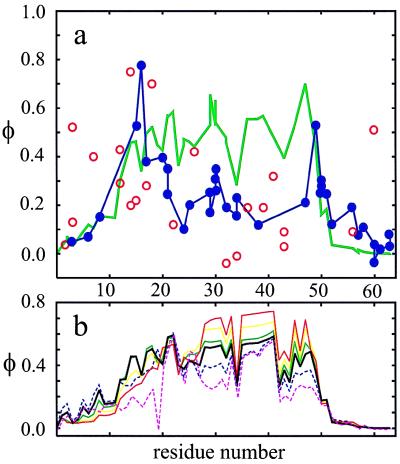
For free energy changes greater than ≈0.25 kcal⋅mol⁻¹, the model predicts that φ values for CI2 become dependent on the size of the perturbation (Fig. 6b). They also depend on whether the mutation is stabilizing or destabilizing.

Figure 6.

Theoretical calculation of φ values. (a) Comparison of experimental and theoretical φ values for CI2. The experimental uncertainty in the φ values arises mainly from the uncertainty in the determination of the folding equilibrium constants. The φ values reported by Itzhaki et al. (40) were therefore divided into two groups according to the absolute magnitude of the change in folding free energy introduced by the mutation (at 4 M urea, the midpoint of the unfolding transition for the wild type). One group (filled blue circles) corresponds to φ values for mutations that cause folding free energy changes >1 kcal⋅mol⁻¹ compared with wild-type whereas the second group (open red circles) corresponds to φ values for mutations that cause free energy changes <1 kcal⋅mol⁻¹. In this second group, there are five negative φ values and one value >1.0, which are not plotted. Also, the value plotted for residue 16 is the one redetermined by Ladurner et al. (41). A blue line connects the filled blue circles to indicate that these values are, for the most part, better determined. Large changes in folding free energy can, however, change the φ value by changing the shape as well as the size of the free energy barrier. To investigate this effect, we used our model to calculate the dependence of the φ value for CI2 on the magnitude of the free energy change (b). These calculations show that the difference between the theoretical φ value calculated using the measured free energy change and the theoretical φ value calculated in the small perturbation limit (see Methods) is <0.1 for all residues except 29 and 47. (b) Dependence of theoretical φ values on the magnitude and sign of the free energy change produced by a mutation. The thick black line corresponds to φ values in the small perturbation limit. Dashed lines are φ values for mutations that stabilize the native state (magenta for |ΔΔG| = 3 kcal⋅mol⁻¹; blue for |ΔΔG| = 1.5 kcal⋅mol⁻¹), and continuous lines are for mutations that destabilize the native state (green for |ΔΔG| = 1.5 kcal⋅mol⁻¹; yellow for |ΔΔG| = 3 kcal⋅mol⁻¹; red for |ΔΔG| = 4.5 kcal⋅mol⁻¹).

RESULTS AND DISCUSSION

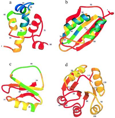
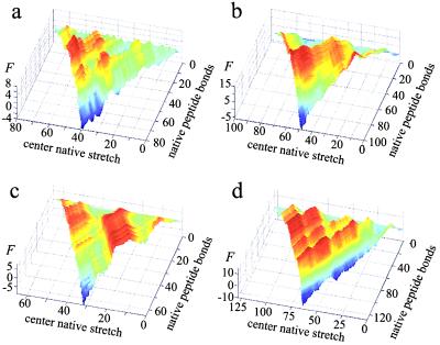
We show two-dimensional free energy surfaces calculated using the single sequence approximation for four proteins: monomeric λ repressor, one of the fastest folding two-state proteins, muscle acyl phosphatase, the slowest two-state folder, CI2, the most intensively studied two-state protein, and Che Y, a protein with a well characterized intermediate (Figs. 2 and 3). The advantage of the single sequence approximation is that it permits easy visualization of the equilibrium properties because the free energy is a function of only two coordinates, the first residue of the native stretch (i) and the number of peptide bonds in the stretch (j). For monomeric λ repressor, muscle acyl phosphatase, and CI2, there are only two deep minima on their free energy surfaces, one for the denatured state and one for the native state, immediately explaining their equilibrium and kinetic two-state behavior. For Che Y, there is an additional minimum that is predicted to be well populated in kinetic experiments. In the predicted intermediate, the N-terminal region, including the first two helices, is folded whereas the C-terminal end is unstructured, in agreement with experiments (31). These surfaces also convey a picture of local regions of structure forming and melting in different parts of the protein. For example, the N-terminal helix of CI2 runs up against a high free energy barrier (the large red mountain) and, in the single sequence approximation, has to melt to find its way between the large (red) mountains to reach the native state (blue valley). In the double (or triple) sequence approximation, native structure can be simultaneously present in two (or three) different regions of the protein. An N-terminal structure can now fuse with a structure formed distal to it to overcome the free energy barrier. This barrier is both broad and bumpy, as suggested from experiments (32).

Figure 2.

Structures of monomeric λ repressor (a), muscle acyl phosphatase (b), CI2 (c), and Che Y (d) showing by the color code the theoretical φ values for each position in the protein (see text). The φ values increase with decreasing wavelength, from red (φ = 0) to yellow (φ = 0.5) to blue (φ = 1). These φ values are calculated in the small perturbation limit, i.e., ΔRTlnK = 0.1 kcal⋅mol⁻¹. The φ value pattern in Che Y requires some explanation because it is a three-state protein. The experiments report the φ values from unfolding kinetics (30) whereas the calculation shown here is for the folding rate from the completely denatured state. Because the N-terminal subdomain is already folded in the intermediate, the folding rate (i.e., the smaller eigenvalue) is insensitive to mutations in this area since they affect the intermediate and the transition state equally.

Figure 3.

Free energy surfaces for monomeric λ repressor (a), muscle acyl phosphatase (b), CI2 (c), and Che Y (d). This surface is the free energy as a function of the number of native peptide bonds (j) and the position of the central residue of a contiguous stretch of native peptide bonds starting at residue i. The free energies increase with increasing wavelength from low (blue) to high (red).

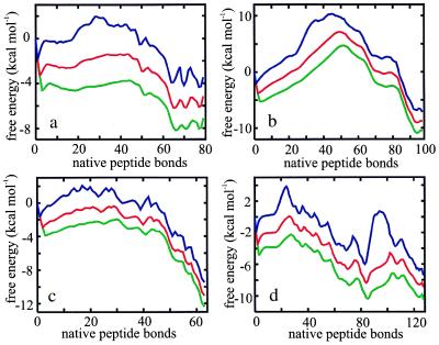
Two-state behavior, bumpy broad barriers, and the existence of partially folded intermediates are more readily seen in plots of the free energy as a function of just the number of native peptide bonds (Fig. 4). This projection of the free energy was done in the single, double, and triple sequence approximations. For all 18 proteins known to exhibit two-state equilibrium and kinetic behavior, there are two deep minima in these free energy profiles, corresponding to the native and denatured states (see supplementary material on the PNAS web site, www.pnas.org).† However, three proteins (CspA, CspB, and SH3 domain from Src), classified as two state proteins (3), have free energy profiles that suggest that partially folded intermediates might be observable in either folding or unfolding experiments. Additional deep minima that should be observed in kinetic experiments are found for ubiquitin, barnase, and the B1 domain of protein G, three proteins that show clear experimental evidence for intermediates (33–35) (see supplementary material).

Figure 4.

Free energy profiles for monomeric λ repressor (a), muscle acyl phosphatase (b), CI2 (c), and Che Y (d). Profiles are shown in the single (blue, upper curve), double (red, middle curve), and triple (green, lower curve) sequence approximations.

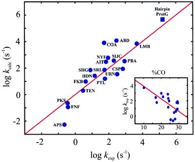
If the number of native bonds is a good reaction coordinate and our free energy is accurate, the dynamics on these one-dimensional free energy profiles should reproduce the experimental folding rates. We calculated the rates from the solution to a one-dimensional diffusion equation (Eq. 4) (28) using the same diffusion coefficient for all proteins. Fig. 5 compares the calculated and observed rates for the 18 two-state proteins in the double sequence approximation. Considering the simplicity of the model, the agreement is remarkably good (correlation coefficient is 0.85). We also found that the rate calculated for the 16-residue β-hairpin from protein GB1, using the same parameters as for the proteins, is very close to the experimental value (Fig. 5).

Figure 5.

Comparison of calculated and experimentally observed folding rates at zero denaturant concentration in the double sequence approximation. The observed rates are taken from the compilation by Jackson (3). The correlation coefficient in the single, double, and triple sequence approximations are 0.83, 0.85, and 0.87, respectively. In the first two, the parameters of the model were adjusted to maximize the agreement by using a least squares criterion. The rates in the triple sequence approximation were calculated with the values of the two Δs_k’s and D from the double sequence approximation, and a new set of ɛ’s in order to reproduce the experimental equilibrium constants. A plot of the experimental log k_f versus log K gives a correlation coefficient of 0.25, showing no significant correlation between folding rate and thermodynamic stability in this set of proteins. The inset shows a plot of the experimental rates versus the percent contact order (%CO) calculated using 0.4 nm as the cut-off-distance for the 18 two-state proteins of our study. The percent contact order defined by Plaxco et al. (19) is

where N is the total number of contacts, ΔS_i,j is the sequence separation in residues between contacting residues i and j, and L is the total number of residues in the protein. The correlation coefficient is 0.64. The folding rate for the β-hairpin extrapolated from the least-squares line is almost 10⁸× smaller than the experimental value. Without the length normalization (L), however, the extrapolated rate is only 30× slower.

The success of these calculations suggests that the range of folding rates found in proteins can be largely explained as a simple competition between conformational entropy loss and stabilization energy from inter-residue interactions. According to our model, structure grows locally. Consequently, proteins with more and stronger local stabilizing interactions immediately compensate the conformational entropy loss as local structure forms, resulting in smaller free energy barriers and faster folding. Similarly, in proteins with more long range interactions, there are fewer stabilizing interactions as the chain organizes in localized regions, resulting in less initial compensation of the conformational entropy loss and a larger free energy barrier. In this way, the model gives a mechanistic explanation for the significant correlation of experimental rates and the mean separation in sequence between contacting residues in the native structure—the contact order of Plaxco et al. (19) (Fig. 5 Inset). Baker and coworkers give a similar explanation of the correlation, using an extension of the analytical model of Zwanzig (19, 22, 36). We should point out that the contact order does not take into account the strength of the interresidue interactions. The importance of the strength as well as the distribution of interactions in determining free energy barrier heights is suggested by the better correlation between our calculated and experimental rates than between the contact order and experimental rates (correlation coefficient = 0.64) (Fig. 5), as well as between the contact order and calculated rates (correlation coefficient = 0.50; plot not shown).

We can also use our model to examine the effect of mutations on the folding rates, as has been done in several previous calculations of free energy surfaces by Wolynes and coworkers (17, 18). The quantity of interest is the relative effect of the mutation on the folding rate and equilibrium constant, defined as φ ≡ Δlnk_f/ΔlnK. A φ value of 1.0 is interpreted as indicating that the structural environment around the residue in the transition state ensemble is identical to the native structure whereas a φ value of zero indicates that it is identical to the structures of the denatured state. However, for the great majority of mutations, the φ values are intermediate between 0 and 1, making the structural interpretation less straightforward (17, 18, 37–39). Fig. 6 shows the results of these calculations for CI2, the protein for which there is the most extensive mutation data from the work of Fersht and coworkers (40). The model gives reasonable agreement with the well determined experimental φ values (filled circles in Fig. 6a) for residues in the regions 1–20, which contains most of the α-helix, and 49–64, which contains the last two β-strands. However, it overestimates the φ values between residues 21 and 47, made up of the second β-strand and the large loop. There are two possible reasons for this. One is a simple counting argument: i.e., restricting the number of simultaneous segments of native structure in each molecule overestimates the probability of finding segments that include residues in the central portion of the sequence. The second is that, in our model, the only way to make contacts between the α-helix and the C-terminal region is for all of the intervening peptide bonds to be in a native conformation whereas in the transition state of the real protein there could be disorder in the connecting β-strand and long loop (Fig. 2). Overall, the agreement between theoretical and experimental φ values is better than could be expected, considering that we are using a highly simplified free energy function.

The model has clearly omitted several factors believed to be important in protein folding. It is straightforward to use more realistic treatments of inter-residue interactions and of the conformational entropy, to include residue propensities for backbone dihedral angles, and to make no restrictions on the allowed number of local regions of native structure in each molecule. It is not so straightforward to include other important effects, such as the contribution of solvent to the free energy barrier, side chain entropy, the role of compactness of the denatured state, and non-native interactions. The effect of non-native interactions should be reflected in the effective diffusion constant used in calculating the dynamics on the one-dimensional profiles (14). One might expect that the diffusion constant would differ for each protein and may account for some of the noise in the calculated rates. Finally, adding native interactions between residues in different stretches would add considerable flexibility to possible structural mechanisms by producing additional routes between the denatured and native states.

A major advantage of the formulation of our model is that it lends itself to a detailed kinetic analysis. Rotation of peptide bonds to native values is both the reaction coordinate of the free energy landscape approach used here and the elementary step in a full kinetic description, equivalent to what was done for the β-hairpin (21). Although for a protein it is not possible to integrate the 2ⁿ differential equations, the calculation can be accomplished with stochastic kinetic algorithms that produce multiple trajectories for individual molecules. These calculations should be useful for testing the accuracy of the single, double, and triple sequence approximations. Only after such tests and better agreement with experimental data is achieved will it be worthwhile to draw conclusions from the wealth of structural and mechanistic detail that is generated by the model.

ABBREVIATION

CI2

chymotrypsin inhibitor 2

References

- 1.Lansbury P T. Proc Natl Acad Sci USA. 1999;96:3342–3344. doi: 10.1073/pnas.96.7.3342. [DOI] [PMC free article] [PubMed] [Google Scholar]
- 2.Jackson S E, Fersht A R. Biochemistry. 1991;30:10428–10435. doi: 10.1021/bi00107a010. [DOI] [PubMed] [Google Scholar]
- 3.Jackson S E. Fold Des. 1998;3:R81–R91. doi: 10.1016/S1359-0278(98)00033-9. [DOI] [PubMed] [Google Scholar]
- 4.Bryngelson J D, Wolynes P G. Proc Natl Acad Sci USA. 1987;84:7524–7528. doi: 10.1073/pnas.84.21.7524. [DOI] [PMC free article] [PubMed] [Google Scholar]
- 5.Onuchic J, Luthey-Schulten A, Wolynes P G. Annu Rev Phys Chem. 1997;48:545–600. doi: 10.1146/annurev.physchem.48.1.545. [DOI] [PubMed] [Google Scholar]
- 6.Shakhnovich E I. Curr Opin Struct Biol. 1997;7:29–40. doi: 10.1016/s0959-440x(97)80005-x. [DOI] [PubMed] [Google Scholar]
- 7.Pande V S, Grosberg A Y, Tanaka T, Rokhsar D S. Curr Opin Struct Biol. 1998;8:68–79. doi: 10.1016/s0959-440x(98)80012-2. [DOI] [PubMed] [Google Scholar]
- 8.Dobson C M, Sali A, Karplus M. Angew Chem Int Edit Engl. 1998;37:868–893. doi: 10.1002/(SICI)1521-3773(19980420)37:7<868::AID-ANIE868>3.0.CO;2-H. [DOI] [PubMed] [Google Scholar]
- 9.Chan H S, Dill K A. Proteins. 1998;30:2–33. doi: 10.1002/(sici)1097-0134(19980101)30:1<2::aid-prot2>3.0.co;2-r. [DOI] [PubMed] [Google Scholar]
- 10.Brooks C L., III Curr Opin Struct Biol. 1998;8:222–226. doi: 10.1016/s0959-440x(98)80043-2. [DOI] [PubMed] [Google Scholar]
- 11.Garel T, Orland H, Pitard E. In: Spin Glasses and Random Fields. Young A P, editor. Singapore: World Scientific; 1998. pp. 387–443. [Google Scholar]
- 12.Hao M H, Scheraga H A. Acc Chem Res. 1998;31:433–440. [Google Scholar]
- 13.Thirumalai D, Klimov D. Curr Opin Struct Biol. 1999;9:197–207. doi: 10.1016/S0959-440X(99)80028-1. [DOI] [PubMed] [Google Scholar]
- 14.Socci N D, Onuchic J N, Wolynes P G. J Chem Phys. 1996;104:5860–5868. [Google Scholar]
- 15.Klimov D K, Thirumalai D. Phys Rev Lett. 1997;79:317–320. [Google Scholar]
- 16.Bryngelson J D, Wolynes P G. J Phys Chem. 1989;93:6902–6915. [Google Scholar]
- 17.Shoemaker B A, Wang J, Wolynes P G. Proc Natl Acad Sci USA. 1997;94:777–782. doi: 10.1073/pnas.94.3.777. [DOI] [PMC free article] [PubMed] [Google Scholar]
- 18.Shoemaker B A, Wang J, Wolynes P G. J Mol Biol. 1999;287:657–694. doi: 10.1006/jmbi.1999.2612. [DOI] [PubMed] [Google Scholar]
- 19.Plaxco K W, Simons K T, Baker D. J Mol Biol. 1998;277:985–994. doi: 10.1006/jmbi.1998.1645. [DOI] [PubMed] [Google Scholar]
- 20.Muñoz V, Thompson P A, Hofrichter J, Eaton W A. Nature (London) 1997;390:196–199. doi: 10.1038/36626. [DOI] [PubMed] [Google Scholar]
- 21.Muñoz V, Henry E R, Hofrichter J, Eaton W A. Proc Natl Acd Sci USA. 1998;95:5872–5879. doi: 10.1073/pnas.95.11.5872. [DOI] [PMC free article] [PubMed] [Google Scholar]
- 22.Zwanzig R. Proc Natl Acd Sci USA. 1995;92:9801–9804. doi: 10.1073/pnas.92.21.9801. [DOI] [PMC free article] [PubMed] [Google Scholar]
- 23.Kabsch W, Sander C. Biopolymers. 1983;22:2577–2637. doi: 10.1002/bip.360221211. [DOI] [PubMed] [Google Scholar]
- 24.Chakrabartty A, Baldwin R L. Adv Protein Chem. 1995;46:141–176. [PubMed] [Google Scholar]
- 25.Muñoz V, Serrano L. Nat Struct Biol. 1994;1:399–409. doi: 10.1038/nsb0694-399. [DOI] [PubMed] [Google Scholar]
- 26.Thompson, P. A., Muñoz, V., Jas, E. R., Henry, E. R., Eaton, W. A. & Hofrichter, J. (1999) J. Phys. Chem., in press.
- 27.Plotkin S S, Wang J, Wolynes P G. J Chem Phys. 1997;106:2932–2948. [Google Scholar]
- 28.Szabo A, Schulten K, Schulten Z. J Chem Phys. 1980;72:4350–4357. [Google Scholar]
- 29.Eaton W A. Proc Natl Acad Sci USA. 1999;96:5897–5899. doi: 10.1073/pnas.96.11.5897. [DOI] [PMC free article] [PubMed] [Google Scholar]
- 30.López-Hernández E, Serrano L. Fold Des. 1996;1:43–55. [PubMed] [Google Scholar]
- 31.López-Hernández E, Cronet P, Serrano L, Muñoz V. J Mol Biol. 1997;266:610–620. doi: 10.1006/jmbi.1996.0793. [DOI] [PubMed] [Google Scholar]
- 32.Oliveberg M, Tan Y J, Silow M, Fersht A R. J Mol Biol. 1998;277:933–943. doi: 10.1006/jmbi.1997.1612. [DOI] [PubMed] [Google Scholar]
- 33.Bycroft M, Matouschek A, Kellis J T, Serrano L, Fersht A R. Nature (London) 1990;346:488–490. doi: 10.1038/346488a0. [DOI] [PubMed] [Google Scholar]
- 34.Khorasanizadeh S, Peters I D, Roder H. Nat Struct Biol. 1996;3:193–205. doi: 10.1038/nsb0296-193. [DOI] [PubMed] [Google Scholar]
- 35.Park, S.-H., Shastry, M. C. R. & Roder, H. (1999) Nat. Struct. Biol., in press. [DOI] [PubMed]
- 36.Alm E, Baker D. Curr Opin Struct Biol. 1999;9:189–196. doi: 10.1016/S0959-440X(99)80027-X. [DOI] [PubMed] [Google Scholar]
- 37.Fersht A R, Matouschek A, Serrano J Mol Biol. 1992;224:771–782. doi: 10.1016/0022-2836(92)90561-w. [DOI] [PubMed] [Google Scholar]
- 38.Fersht A R. Structure and Mechanism in Protein Science: A Guide to Enzyme Catalysis and Protein Folding. New York: Freeman; 1998. [Google Scholar]
- 39.Onuchic J, Socci N D, Luthey-Schulten Z, Wolynes P G. Fold Des. 1996;1:441–450. doi: 10.1016/S1359-0278(96)00060-0. [DOI] [PubMed] [Google Scholar]
- 40.Itzhaki L S, Otzen D E, Fersht A R. J Mol Biol. 1995;254:260–288. doi: 10.1006/jmbi.1995.0616. [DOI] [PubMed] [Google Scholar]
- 41.Ladurner A G, Itzhaki L S, Fersht A R. Fold Des. 1997;2:363–368. doi: 10.1016/S1359-0278(97)00050-3. [DOI] [PubMed] [Google Scholar]
Associated Data
This section collects any data citations, data availability statements, or supplementary materials included in this article.