Finite Element Analysis of the Time-Dependent Smoluchowski Equation for Acetylcholinesterase Reaction Rate Calculations

Abstract

This article describes the numerical solution of the time-dependent Smoluchowski equation to study diffusion in biomolecular systems. Specifically, finite element methods have been developed to calculate ligand binding rate constants for large biomolecules. The resulting software has been validated and applied to the mouse acetylcholinesterase (mAChE) monomer and several tetramers. Rates for inhibitor binding to mAChE were calculated at various ionic strengths with several different time steps. Calculated rates show very good agreement with experimental and theoretical steady-state studies. Furthermore, these finite element methods require significantly fewer computational resources than existing particle-based Brownian dynamics methods and are robust for complicated geometries. The key finding of biological importance is that the rate accelerations of the monomeric and tetrameric mAChE that result from electrostatic steering are preserved under the non-steady-state conditions that are expected to occur in physiological circumstances.

INTRODUCTION

Diffusion plays an important role in a variety of biomolecular processes, which have been studied extensively using various biophysical, biochemical, and computational methods. Computational models of diffusion have been widely studied using both discrete (1–5) and continuum methods (6–11). The discrete methods concentrate on the stochastic processes based on individual particles, which include Monte Carlo (5,12–14), Brownian dynamics (BD) (15–17), and Langevin dynamics (18,19) simulations. Continuum modeling describes the diffusional processes via concentration distribution probability in lieu of stochastic dynamics of individual particles. Comparing with the discrete methods, continuum approaches need not deal with the individual Brownian particles and the computational cost can be substantially less than for the discrete methods.

In previous work with continuum methods, Song et al. (9,10) have presented finite element methods for solving the steady-state Smoluchowski equation (SSSE), which describes the steady-state behavior of diffusion-limited ligand binding. These methods have been shown to be significantly more efficient than traditional BD approaches for evaluating reaction rate constants for diffusion-limited binding of simple ligands. Recently, Zhang et al. (20) applied this approach for studies of several conformations of tetrameric mouse acetylcholinesterase (mAChE). However, the SSSE solution only provides the answer at the time-independent stage of diffusion. In other words, we only obtain the concentration distribution and rate constant when diffusion and reaction between the ligand and the enzyme reach the steady state. Physiological conditions, however, can be expected to include non-steady-state kinetics. One possible way to study the diffusion dynamics on biomolecular interface binding energy landscape is mean first-passage time, which was introduced recently by Wang et al. (21). The theory suggests a way of connecting the models/simulations with single molecule experiments by analyzing the kinetic trajectories. However, it is still an open question for the diffusional problem in a large spatial and timescale.

In the present work, we apply adaptive finite element methods to solve the time-dependent Smoluchowski equation (TDSE), using a posteriori error estimation to iteratively refine the finite element meshes. The binding of charged and noncharged ligands to mAChEs has been described at each timestep. The diffusion results have been compared with those from steady-state Smoluchowski diffusion studies and experimental results. AChE is a serine esterase that terminates the activity of acetylcholine (ACh) within cholinergic synapses by hydrolysis of the ACh ester bond to produce acetate and choline (22). Hydrolysis of ACh occurs in the active site of AChE, which lies at the base of a 20 Å-deep gorge within the enzyme. The rate-limiting step of ACh hydrolysis by AChE is the diffusional encounter (23–25), making the system a popular target for both experimental (26–28) and computational diffusion studies (29,30).

THEORY AND MODELING DETAILS

Our time-dependent SMOL solver (http://mccammon.ucsd.edu/smol/index.html) models the diffusion of ligands relative to a target molecule, subject to a potential obtained by solving the Poisson-Boltzmann equation. It is perhaps most easily explained by initially considering motion of an ensemble of Brownian particles in a prescribed external potential (R→ being a particle's position) under conditions of high friction, where the Smoluchowski equation applies.

Boundaries and initialization of the time-dependent Smoluchowski equation

The starting point for development of the time-dependent SMOL solver is the steady-state SMOL solver described by Song et al. (9,10). The original Smoluchowski equation has the form of a continuity equation,

(1)

where the particle flux is defined as

(2)

Here is the distribution function of the ensemble of Brownian particles, is the diffusion coefficient, β = 1/k_BT is the inverse Boltzmann energy, k_B is the Boltzmann constant, T is the temperature, and is the potential of mean force (PMF) for a diffusing particle due to solvent-mediated interactions with the target molecule. For simplicity, can be assumed constant. The two terms contributing to the flux have clear physical meanings. The first is due to free diffusional processes, as quantified by Fick's first law. The second contribution is due to the drift velocity, , induced by the systematic forces, , and friction quantified by the friction constant γ. The relation between diffusion coefficient D and friction constant γ is given by Stokes-Einstein equation: Dβγ = 1.

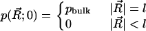
The TDSE can be solved to determine biomolecular diffusional encounter rates before steady state is established. Following the work of Song et al. (9,10) and Zhou et al. (31–33), the application of the TDSE to this question involves the solution of Eq. 1 in a three-dimensional domain Ω, with the following boundary and initial conditions. A bulk Dirichlet condition is imposed on the outer boundary Γ_b ⊂ ∂Ω,

(3)

where p_bulk denotes the bulk concentration at the outer boundary. A reactive Robin condition is implemented on the active site boundary Γ_a ⊂ ∂Ω,

(4)

providing an intrinsic reaction rate . Here, is the surface normal. For the diffusion-limited reaction process, such as ACh hydrolysis by mAChE, the concentration of ACh at the binding site is approximately zero. Therefore, the reactive Robin condition on the inner boundary can be simplified as

(5)

For the nonreactive surface parts of the inner boundary Γ_r ⊂ ∂Ω, a reflective Neumann condition is employed:

(6)

Finally, we set up the initial conditions as

(7)

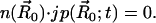
Therefore, the diffusion-determined biomolecular reaction rate constant during the simulation time can be obtained from the flux by integration over the active site boundary, i.e.,

(8)

Finite element discrete formulation

To numerically solve the TDSE, we employed the Galerkin finite element approximation to discretize the differential equation (34). The original TDSE (Eq. 1) can be written as described below (10,35,36).

Let Ω ⊂ R³ be an open set, and let ∂Ω denote the boundary, which can be thought of as a set in R². Consider now the TDSE, a member of the class of elliptic equations

(9)

where 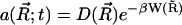and .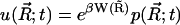

According to Holst et al. (37), the solution to the original problem also solves the problem

(10)

where u is the approximate solution found by the numerical method, ū is a trace function satisfying the Dirichlet boundary conditions, and is the test function space (37,38). The “weak” bilinear form 〈F(u), v〉 is given by

(11)

We have used the fact that a boundary integral vanishes because the test function v vanishes on the boundary.

For a discrete solution to Eq. 11, taking span{φ₁, φ₂, …, φ_N} ⊂ , Eq. 11 reduces to a set of N nonlinear algebraic relations (implicitly defined) for N coefficients {α_j} in the expansion:

(12)

According to the Galerkin approximation, N equals the number of finite element nodes.

Therefore, the corresponding “weak form” of the TDSE is

(13)

To obtain an unconditionally stable solution, two implicit algorithms have been implemented in our codes: Crank-Nicolson and backward Euler's methods.

Finally, the concentration distribution can be obtained by .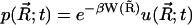

A posteriori error estimation and mesh refinement

As described by Holst et al. (37), the adaptive mesh refinement procedure follows a solve-estimate-refine algorithm and has been implemented in the FEtk software (http://www.fetk.org/). Because of the inefficiency to “estimate” and “refine” in each time step, we only estimated and refined the mesh while solving the SSSE. With the refined mesh, TDSE diffusion studies were implemented. In the “estimate” step, we introduced the a posteriori error estimator η_s below holding for a Galerkin approximation u_h satisfying

(14)

where C₀ is a constant and the element-wise error indicator η_s is defined as

(15)

where h_s and h_f represent the diameter of the simplex s and the face f, respectively. The expression f ∈ s denotes a face of simplex, [v]_f denotes the jump across the face of function v, and the Lebesgue norm is

(16)

The entire “solve-estimate-refine” cycle is repeated until the global error is reduced to an acceptable user-defined level.

Potential of mean force (PMF) input

Currently we provide two options to map the PMF to each finite element node in the time-dependent SMOL solver code. First, it can input the PMF obtained by boundary element methods (39,40). The PMF corresponds to the electrostatic potential obtained by solving the Poisson-Boltzmann equation. Second, APBS 0.4.0 (http://sourceforge.net/projects/apbs) is used to calculate the PMF, which is the potential field W(r) in Eq. 2 (36). The partial charges and radii of each atom in the mAChE monomer and tetramer molecules have been assigned using the CHARMM22 force field, and the dielectric constant is set as 4.0 inside the protein and 78.0 for the solvent. The solvent probe radius is set as 1.4 Å, and the ion exclusion layer is set as 2.0 Å. Ionic strengths varying between 0 and 0.67 M were used in the PMF calculations and following diffusion studies.

To allow the potential to approach zero at the outer boundary, a large space of 40 times the radius of the biomolecule is required. A series of nested potential grids is constructed in a multiresolution format where higher resolution meshes provide PMF values near the molecular surface while coarser meshes are used away from the molecule. The dimensions of the finest grid are given by the psize.py utility in the APBS software package, and the coarsest grid dimensions are set to cover the whole problem domain plus two grid spacings (to allow gradient calculation) in each dimension. The setup for the rest of the grid hierarchy is calculated using a geometric sequence for grid spacing. For mAChE monomer, the finest grid has dimensions of 86.3 Å × 76.4 Å × 101.4 Å with 161, 129, and 193 grid points in each direction, respectively. This corresponds to a 0.5 Å × 0.6 Å × 0.5 Å grid spacing setup. The coarsest grid has dimensions of 3400 Å × 3000 Å × 4300 Å with 161 grid points in each direction. The corresponding grid spacing settings are 21.1 Å × 18.6 Å × 26.7 Å.

Adaptive finite element mesh generation

For the mAChE monomer case, similarly with previous studies (9,10), we used a mouse AChE (mAChE) structure adapted from the crystal structure of the mAChE-fasciculin II complex (26) and perturbed by Tara and co-workers via molecular dynamics simulations with an ACh-like ligand in the active site gorge (30) to produce gorge conformations with wider widths than the original x-ray structure. The diffusing ligand was modeled as a sphere with an exclusion radius of 2.0 Å and a diffusion constant of 7.8 × 10⁴ Ų/μs. This perturbation was necessary for computational diffusion simulations with a fixed biomolecular structure. Reactive boundaries were defined using the biomolecular surface, which is the same as that used in Song et al. (10).

For the mAChE tetramer cases, we used three structures: a loose, pseudo-square planar tetramer with antiparallel alignment of the two four-helix bundles and a large space in the center (PDB: 1C2B); a compact, square nonplanar tetramer with parallel arrangement of the four-helix bundles that may expose all the four t peptide sequences on a single side (PDB: 1C2O); and in addition to the crystal structures, an intermediate structure (INT) was generated by morphing the two crystal structures using the morph script in visual molecular dynamics (41). Reactive boundary definitions are the same as the above mAChE monomer case.

The tetrahedral meshes were obtained and refined from the inflated van der Waals-based accessibility data for the mAChE monomer and tetramers using the level-set boundary interior exterior-mesher (42–44). Initially the region between the biomolecule and a slightly larger sphere centered about the molecular center of mass, was discretized by adaptive tetrahedral meshes. It generated very fine triangular elements near the active site gorge, while coarser elements everywhere else. The mesh is then extended to the entire diffusion domain and the inside of the biomolecule with spatial adaptivity in that the mesh element size increases with increasing distance from the biomolecule. The number of tetrahedral elements varies from 50,000 to 70,000 for different tetramer geometries.

RESULTS AND DISCUSSION

Validation of the time-dependent SMOL code with a spherical test case

Before applying the time-dependent SMOL program to a biomolecular system with complicated geometries, we first tested it with the classic spherical system (45) and compared the calculated result with the known analytical solution. For this test case, we chose a diffusing sphere with a 2 Å radius and neutral charge. The entire problem domain is a sphere with a 400 Å radius, which was discretized with 745,472 tetrahedral elements. A detailed view of the surface mesh for the stationary sphere is also shown in Fig. 1. The time-dependent Smoluchowski equation then becomes the Einstein diffusion equation. The diffusing particle's dimensionless bulk concentration was set to 1. Ignoring hydrodynamic interactions, the diffusion constant D is calculated as 7.8 × 10⁴ Ų/μs using the Stokes-Einstein equation with a hydrodynamic radius of 3.5 Å, solvent viscosity of 0.891 × 10⁻³ kg/(m · s), and 300 K temperature.

FIGURE 1.

Illustration of the discretized problem domain for the spherical analytical test. The green represents the outer boundary, in which the ligand concentration is kept as a constant.

Analytical solution

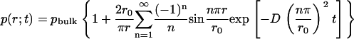
For a spherically symmetric system without external potential, the TDSE can be written as

with boundary conditions

where r₀ is the radius for the outer boundary. The analytical expression for the concentration distribution is

This analytical form of the solution was expressed by the sum of zero-order spherical Bessel functions. Fig. 1 presents the concentration distributions during the simulation time with our TDSE solver, comparing with the above analytical solution.

SMOL numerical solution

According to Fig. 2, the performance of the SMOL program is good, with almost the same concentration distribution as in the analytical solution. It must be noted that the analytical solution for the time-dependent diffusion with the Columbic potential cannot be addressed with a simple formula; however, we have implemented our solver to test the same steady-state case addressed in Table 1 of Song et al. (10), and obtained very consistent results.

FIGURE 2.

Time evolution of the two-dimensional concentration distribution contour in the problem domain. (a) Our SMOL solution; (b) spherical analytical solution.

TABLE 1.

SSSE reaction rate and TDSE final reaction rate constants as a function of ionic strength

Ionic strength (M)	0.000	0.025	0.100	0.300	0.600
SSSE results kon (1011 M−1 min−1)	9.562	3.681	2.304	1.572	1.302
TDSE final results kon (1011 M−1 min−1)	9.535	3.673	2.298	1.569	1.298

Application of the TDSE solver to mouse acetylcholinesterase monomer

One of the major advantages of continuum methods such as the time-dependent SMOL solver is the ability to simulate the complete diffusion dynamics for large biological systems with complicated geometries with significantly lower computational cost than the Brownian dynamics approach. This section demonstrates the implementation of TDSE to study the ligand binding kinetic process of the mAChE monomer under various ionic strength conditions (46).

With the original mesh, we measured the diffusion-controlled reaction rates during the simulation time with the timestep at 50 ps, as shown in Fig. 3. Separate calculations were performed at ionic strengths of 0.000, 0.050, 0.100, 0.150, 0.200, 0.250, 0.300, 0.450, 0.600, and 0.670 M. At the zero ionic strength, the whole system reaches the steady state in over 15 ns. The value of k_on at the end of the simulation is 9.535 × 10¹¹ M⁻¹ · min⁻¹, which is very consistent with the experimental value at (9.80 ± 0.60) × 10¹¹ M⁻¹ · min⁻¹ (27). Meanwhile, the k_on value for the neutral ligand at the steady state is 9.297 × 10¹⁰ M⁻¹ · min⁻¹, which is consistent with the previous steady-state calculations (20). Table 1 (this article) listed the final k_on value derived from the TDSE calculations and the corresponding sets from SSSE calculations (9). When the ionic strength becomes higher, the time to reach the steady state decreases substantially. Obviously, we have obtained consistent results, comparing with the previous SSSE and BD calculations.

FIGURE 3.

k_on(t) values in time-dependent ACh diffusion under the various ionic strength conditions.

Furthermore, our TDSE solver can report all the ligand concentration distribution histories during the 20 μs simulation. In this case, we recorded a concentration distribution every 100 timesteps (5 ns) and a restart checkpoint every 1000 timesteps (50 ns). Fig. 4 demonstrates the two-dimensional concentration distribution around the mAChE molecule at the end of 20 μs simulation. The origin and the normal of the clip plane have been set at (0 16.6 Å 0) and (1 0 1), respectively. The value k_on exhibits an ionic strength-dependence strongly indicative of electrostatic acceleration. The high ionic strength environment lessens the electrostatic interactions between the active site of mAChE and the ligand. Therefore, the relatively low ligand concentration area shrinks while ionic strength increases. Specifically, at 0.150 M ionic strength, several dynamic snapshots have been plotted, as depicted in Fig. 2. These snapshots demonstrate the whole diffusion process of ACh-like ligands from the area far from the enzyme until they reach the active site and react and disappear.

FIGURE 4.

Two-dimensional ligand concentration distribution contour around mAChE at the steady state under various ionic strengths. The red color represents high concentration area, while the blue represents low concentration area.

In this section, we explore the use of the adaptive finite element methods to implement TDSE calculations on the mAChE monomer. The first step is to interactively solve the SSSE based on the a posteriori error estimation (10,37). The iterative error-based refinement of the initial 656,823-simplex mesh was performed until the global error is less than a value chosen to provide reaction rates that did not change appreciably upon further refinement. The refined mesh has 824,746 simplexes at 150 mM ionic strength. Then, we implemented another TDSE calculation with the refined mesh. Fig. 5 shows the kinetic curves of both the original and refined mesh. Again, the two calculations are in good overall agreement but do show some differences at the final steady state. Specifically, the refinement of the adaptive meshes shows a little increase of the k_on value after reaching the steady state.

FIGURE 5.

The time-dependent ligand concentration distribution at 0.150 M ionic strength for the mAChE monomer.

Application of the TDSE solver to mAChE tetramers

A previous SSSE study described the effect of electrostatic forces on ACh steady-state diffusion to the mouse acetylcholinesterase tetramer (20). Here, we extend the previous study using the same meshes and potential files with our time-dependent SMOL solver. The time step for the three tetramer models was set at 10 ns, and concentration histories were recorded every 100 steps. Two crystal structures (1C2O and 1C2B) and an intermediate structure (INT) are all studied by solving the TDSE. The actual conformational dynamics of the mouse acetylcholinesterase tetramer has been neglected in this work.

Fig. 6 a shows the time-dependent rate constant per active site at 0.150 M ionic strength for the above three mouse acetylcholinesterase tetramer structures. It takes >75 μs for each active site to reach the steady state. For structure 1C2O, the entrances to two of the four active gorges (AS2 and AS4) are partially blocked by another subunit in the complementary dimer, while the other two gorges are completely accessible from outside (AS1 and AS3). As a result, the four kinetic curves in 1C2O can be classified into two subgroups: one subgroup corresponds to active site 1 (AS1) and active site 3 (AS3), in each of which the gorge is open, and at the end of the simulation, the reaction rates are 1.61 × 10¹¹ M⁻¹ min⁻¹ and 1.50 × 10¹¹ M⁻¹ min⁻¹, respectively. Another subgroup corresponds to active site 2 (AS2) and active site 4 (AS3), where the gorges are sterically shielded by nearby subunits, and the final reaction rates are 8.47 × 10¹⁰ M⁻¹ min⁻¹ and 9.62 × 10¹⁰ M⁻¹ min⁻¹, respectively, which is a little more than half of that for AS1 or AS3. Fig. 6 b demonstrates the k_on(t) values for the neutral ligand. Comparing with the +1.0e charged ligand, the neutral ligand still shows similar time-dependent curves for individual active sites, while the k_on(t) value is much less than the corresponding +1.0e charged case.

FIGURE 6.

The comparison of k_on values in time-dependent ACh diffusion between the original and refined meshes.

Similarly, we tested the final steady-state concentration distribution in the diffusion domain under various ionic strength conditions for the AChE tetramers. For example, Fig. 8 illustrates the different concentration profiles at 0.025, 0.050, 0.100, 0.300, 0.450, and 0.670 M ionic strength solutions for structure 1C2O. Comparing with the monomer case, the ACh-like ligand concentration around the 1C2O molecule is much lower when the ionic strength is small, due to the stronger electrostatic attraction between the ligands and the tetramer molecule. While the ionic strength becomes higher, the electrostatic effect on the steady-state concentration distribution turns out to be weaker.

FIGURE 8.

Steady-state ligand concentration distribution under six different ionic strength conditions for structure 1C2O.

We also obtained the time-dependent rate constant per active site for the structure 1C2B, in which all the four gorges are nearly completely accessible to the solvent (Fig. 7). The profiles of k_on(t) of AS3 and AS4 are almost the same, while the value of the final steady state for AS1 or AS2 is a little smaller, but still above 1.10 × 10¹¹ M⁻¹ min⁻¹. The sum of the four active sites is 5.28 × 10¹¹ M⁻¹ min⁻¹, whereas the total steady-state k_on in structure 1C2O is 4.92 × 10¹¹ M⁻¹ min⁻¹. It must be noted that the steady-state k_on in the mAChE monomer is 1.97 × 10¹¹ M⁻¹ min⁻¹ at 0.150 M ionic strength. Therefore, the average reaction rate per active site for the tetramer is ∼64% that of the monomer, which is close to the result of the previous SSSE studies (20). The four active sites show similar kinetic profiles, and reach the steady states at nearly the same time. Meanwhile, the time-dependent rate constant per active site in the structure INT appears more like that in the structure 1C2B, although the difference between AS1 and AS3 is still similar with that in the structure 1C2O. Additionally, our time-dependent SMOL solver can show the detailed diffusion process. For the 1C2O case, Fig. 8 describes the ligand concentration distribution in the problem domain. The red represents high concentration areas, while the blue represents the low concentration areas.

FIGURE 7.

The dependency of k_on(t) values on the simulation time for the structures 1C2O, INT, and 1C2B: (a) 0.150 M ionic strength and +1.0e ligand; and (b) neutral ACh-like ligand.

CONCLUSIONS

In this study, we describe new continuum-based methods for studying diffusion in biomolecular systems. Specifically, we present the time-dependent SMOL software package, a finite element-based set of tools for solving the TDSE to calculate ligand binding rate constants for large biomolecules under pre-steady-state and steady-state conditions. The main improvement from the previous SMOL solver (9,10) can be addressed as below: first, the new solver has removed the drift term (Eq. 2) which is discontinuous for ∇W, as well as the asymmetry (47). Theoretically, the new SMOL solver can utilize the conjugate gradient method, which is a direct method for symmetric and positive definite linear systems, while the old solver can only solve SSSE with the bi-conjugate gradient method. Compared with the new solver, the bi-conjugate gradient method is slower and harder to converge. Therefore, our new SMOL solver can solve both steady-state and time-dependent problems much more efficiently and stably than the old version.

With the new code, we solved the time-dependent diffusion in the analytical case of a reactive sphere, mAChE monomer and tetramer cases. Comparing with previous steady-state studies, our research extends the study into the nonequilibrium diffusion dynamics and obtained very consistent results. Moreover, the calculated rates of the mAChE monomer were compared with experimental data (27) and show very good agreement with experiment while requiring substantially less computational effort than existing particle-based Brownian dynamics methods. Additionally, the value of k_on(t) seems to be underestimated with the coarser meshes, which is consistent with previous observations (10). Similarly, the k_on values in mAChE tetramers should increase if we refine the original mesh. In the previous study (20) and this one, we have found the activity of one subunit in a mAChE tetramer equals ∼60–70% that of a free monomer. With the appropriate meshes, we would expect to obtain an activity closer to that in the free monomer and the catalytic activity might not be too affected by subunit association as suggested in the experiment (48).

Additionally, we describe new adaptive meshing methods developed to discretize biomolecular systems into finite element meshes, which respect the geometry of the biomolecule. Although not presented in this study, it is important to note that the new meshing methods could be useful in a variety of biological simulations including computational studies of biomolecular electrophoresis (49), elasticity (42,43), and electrostatics (35,36,50,51).

Finally, this research lays the groundwork for the integration of molecular-scale information into simulations of cellular-scale systems such as the neuromuscular junction (6,11,52). In particular, this new finite element framework should facilitate the incorporation of other continuum mechanics phenomena into biomolecular simulations. The ultimate goal of this work is to develop scalable methods and theories that will allow researchers to begin to study biological dynamics in a cellular context efficiently and robustly.

FIGURE 9.

Ligand concentration distribution in the diffusion domain during the simulation time for structure 1C2O.

References

- 1.Ermak, D. L., and J. A. McCammon. 1978. Brownian dynamics with hydrodynamic interactions. J. Chem. Phys. 69:1352–1360. [Google Scholar]
- 2.Northrup, S. H., S. A. Allison, and J. A. McCammon. 1984. Brownian dynamics simulation of diffusion-influenced bimolecular reactions. J. Chem. Phys. 80:1517–1526. [Google Scholar]
- 3.Agmon, N., and A. L. Edelstein. 1997. Collective binding properties of receptor arrays. Biophys. J. 72:1582–1594. [DOI] [PMC free article] [PubMed] [Google Scholar]
- 4.Gabdoulline, R. R., and R. C. Wade. 1998. Brownian dynamics simulation of protein-protein diffusional encounter. Methods. 14:329–341. [DOI] [PubMed] [Google Scholar]
- 5.Stiles, J. R., and T. M. Bartol. 2000. Monte Carlo methods for simulating realistic synaptic microphysiology using MCell. In Computational Neuroscience: Realistic Modeling for Experimentalists. E. D. Schutter, editor. CRC Press, New York.
- 6.Smart, J. L., and J. A. McCammon. 1998. Analysis of synaptic transmission in the neuromuscular junction using a continuum finite element model. Biophys. J. 75:1679–1688. [DOI] [PMC free article] [PubMed] [Google Scholar]
- 7.Kurnikova, M. G., R. D. Coalson, P. Graf, and A. Nitzan. 1999. A lattice relaxation algorithm for three-dimensional Poisson-Nernst-Planck theory with application to ion transport through the Gramicidin A channel. Biophys. J. 76:642–656. [DOI] [PMC free article] [PubMed] [Google Scholar]
- 8.Schuss, Z., B. Nadler, and R. S. Eisenberg. 2001. Derivation of Poisson and Nernst-Planck equations in a bath and channel from a molecular model. Phys. Rev. E. 64:036116. [DOI] [PubMed] [Google Scholar]
- 9.Song, Y. H., Y. J. Zhang, C. L. Bajaj, and N. A. Baker. 2004. Continuum diffusion reaction rate calculations of wild-type and mutant mouse acetylcholinesterase: adaptive finite element analysis. Biophys. J. 87:1558–1566. [DOI] [PMC free article] [PubMed] [Google Scholar]
- 10.Song, Y. H., Y. J. Zhang, T. Y. Shen, C. L. Bajaj, A. McCammon, and N. A. Baker. 2004. Finite element solution of the steady-state Smoluchowski equation for rate constant calculations. Biophys. J. 86:2017–2029. [DOI] [PMC free article] [PubMed] [Google Scholar]
- 11.Tai, K. S., S. D. Bond, H. R. Macmillan, N. A. Baker, M. J. Holst, and J. A. McCammon. 2003. Finite element simulations of acetylcholine diffusion in neuromuscular junctions. Biophys. J. 84:2234–2241. [DOI] [PMC free article] [PubMed] [Google Scholar]
- 12.Berry, H. 2002. Monte Carlo simulations of enzyme reactions in two dimensions: fractal kinetics and spatial segregation. Biophys. J. 83:1891–1901. [DOI] [PMC free article] [PubMed] [Google Scholar]
- 13.Genest, D. 1989. A Monte Carlo simulation study of the influence of internal motions on the molecular-conformation deduced from two-dimensional NMR experiments. Biopolymers. 28:1903–1911. [DOI] [PubMed] [Google Scholar]
- 14.Saxton, M. J. 1992. Lateral diffusion and aggregation—a Monte Carlo study. Biophys. J. 61:119–128. [DOI] [PMC free article] [PubMed] [Google Scholar]
- 15.McCammon, J. A. 1987. Computer-aided molecular design. Science. 238:486–491. [DOI] [PubMed] [Google Scholar]
- 16.Northrup, S. H., J. O. Boles, and J. C. L. Reynolds. 1988. Brownian dynamics of cytochrome-c and cytochrome-c peroxidase association. Science. 241:67–70. [DOI] [PubMed] [Google Scholar]
- 17.Wade, R. C., M. E. Davis, B. A. Luty, J. D. Madura, and J. A. McCammon. 1993. Gating of the active-site of triose phosphate isomerase—Brownian dynamics simulations of flexible peptide loops in the enzyme. Biophys. J. 64:9–15. [DOI] [PMC free article] [PubMed] [Google Scholar]
- 18.Eastman, P., and S. Doniach. 1998. Multiple timestep diffusive Langevin dynamics for proteins. Proteins. 30:215–227. [PubMed] [Google Scholar]
- 19.Yeomans-Reyna, L., and M. Medina-Noyola. 2001. Self-consistent generalized Langevin equation for colloid dynamics. Phys. Rev. E Stat. Nonlin. Soft Matter Phys. 64:066114. [DOI] [PubMed] [Google Scholar]
- 20.Zhang, D. Q., J. Suen, Y. J. Zhang, Y. H. Song, Z. Radić, P. Taylor, M. J. Holst, C. Bajaj, N. A. Baker, and J. A. McCammon. 2005. Tetrameric mouse acetylcholinesterase: continuum diffusion rate calculations by solving the steady-state Smoluchowski equation using finite element methods. Biophys. J. 88:1659–1665. [DOI] [PMC free article] [PubMed] [Google Scholar]
- 21.Wang, J. 2006. Diffusion and single molecule dynamics on biomolecular interface binding energy landscape. Chem. Phys. Lett. 418:544–548. [Google Scholar]
- 22.Berg, J. M., J. L. Tymoczko, and L. Stryer. 1995. Biochemistry. W. H. Freeman & Co., New York, NY.
- 23.Bazelyansky, M., E. Robey, and J. F. Kirsch. 1986. Fractional diffusion-limited component of reactions catalyzed by acetylcholinesterase. Biochemistry. 25:125–130. [DOI] [PubMed] [Google Scholar]
- 24.Berman, H. A., K. Leonard, and M. W. Nowak. 1991. Cholinesterases: Structure, Function, Mechanism, Genetics and Cell Biology. J. Massoulie, editor. American Chemical Society, Washington, DC.
- 25.Nolte, H. J., T. L. Rosenberry, and E. Neumann. 1980. Effective charge on acetylcholinesterase active-sites determined from the ionic-strength dependence of association rate constants with cationic ligands. Biochemistry. 19:3705–3711. [DOI] [PubMed] [Google Scholar]
- 26.Bourne, Y., P. Taylor, and P. Marchot. 1995. Acetylcholinesterase inhibition by fasciculin—crystal structure of the complex. Cell. 83:503–512. [DOI] [PubMed] [Google Scholar]
- 27.Radić, Z., D. M. Quinn, J. A. McCammon, and P. Taylor. 1997. Electrostatic influence on the kinetics of ligand binding to acetylcholinesterase—distinctions between active center ligands and fasciculin. J. Biol. Chem. 272:23265–23277. [DOI] [PubMed] [Google Scholar]
- 28.Velsor, L. W., C. A. Ballinger, J. Patel, and E. M. Postlethwait. 2003. Influence of epithelial lining fluid lipids on NO2-induced membrane oxidation and nitration. Free Radic. Biol. Med. 34:720–733. [DOI] [PubMed] [Google Scholar]
- 29.Tan, R. C., T. N. Truong, J. A. McCammon, and J. L. Sussman. 1993. Acetylcholinesterase—electrostatic steering increases the rate of ligand-binding. Biochemistry. 32:401–403. [DOI] [PubMed] [Google Scholar]
- 30.Tara, S., A. H. Elcock, J. M. Briggs, Z. Radić, P. Taylor, and J. A. McCammon. 1998. Rapid binding of a cationic active site inhibitor to wild type and mutant mouse acetylcholinesterase: Brownian dynamics simulation including diffusion in the active site gorge. Biopolymers. 46:465–474. [DOI] [PubMed] [Google Scholar]
- 31.Zhou, H. X. 1990. On the calculation of diffusive reaction-rates using Brownian dynamics simulations. J. Chem. Phys. 92:3092–3095. [Google Scholar]
- 32.Zhou, H. X., S. T. Wlodek, and J. A. McCammon. 1998. Conformation gating as a mechanism for enzyme specificity. Proc. Natl. Acad. Sci. USA. 95:9280–9283. [DOI] [PMC free article] [PubMed] [Google Scholar]
- 33.Zhou, H. X., J. M. Briggs, S. Tara, and J. A. McCammon. 1998. Correlation between rate of enzyme-substrate diffusional encounter and average Boltzmann factor around active site. Biopolymers. 45:355–360. [DOI] [PubMed] [Google Scholar]
- 34.Axelsson, O., and V. A. Barker. 2001. Finite Element Solution of Boundary Value Problems. Theory and Computation. Society for Industrial and Applied Mathematics, Philadelphia, PA.
- 35.Holst, M., N. Baker, and F. Wang. 2000. Adaptive multilevel finite element solution of the Poisson-Boltzmann equation. I. Algorithms and examples. J. Comput. Chem. 21:1319–1342. [Google Scholar]
- 36.Baker, N., M. Holst, and F. Wang. 2000. Adaptive multilevel finite element solution of the Poisson-Boltzmann equation. II. Refinement at solvent-accessible surfaces in biomolecular systems. J. Comput. Chem. 21:1343–1352. [Google Scholar]
- 37.Holst, M. 2001. Adaptive numerical treatment of elliptic systems on manifolds. Adv. Comput. Math. 15:139–191. [Google Scholar]
- 38.Braess, D. 1997. Finite Elements: Theory, Fast Solvers, and Applications in Solid Mechanics. Cambridge University Press, New York, NY.
- 39.Lu, B. Z., X. L. Cheng, T. J. Hou, and J. A. McCammon. 2005. Calculation of the Maxwell stress tensor and the Poisson-Boltzmann force on a solvated molecular surface using hypersingular boundary integrals. J. Chem. Phys. 123:084904. [DOI] [PubMed] [Google Scholar]
- 40.Lu, B. Z., D. Q. Zhang, and J. A. McCammon. 2005. Computation of electrostatic forces between solvated molecules determined by the Poisson-Boltzmann equation using a boundary element method. J. Chem. Phys. 122:214102. [DOI] [PubMed] [Google Scholar]
- 41.Humphrey, W., A. Dalke, and K. Schulten. 1996. VMD: visual molecular dynamics. J. Mol. Graph. 14:33–38. [DOI] [PubMed] [Google Scholar]
- 42.Zhang, Y. J., C. L. Bajaj, and B. S. Sohn. 2003. Adaptive and quality 3-D meshing from imaging data. In Proceedings of the 8th ACM Symposium on Solid Modeling and Applications. ACM Press, Seattle, WA.
- 43.Zhang, Y. J., C. L. Bajaj, and B. S. Sohn. 2004. 3D finite element meshing from imaging data. The special issue of Computer Methods in Applied Mechanics and Engineering (CMAME) on Unstructured Mesh Generation. CMAME. 194:5083–5106. [DOI] [PMC free article] [PubMed] [Google Scholar]
- 44.Zhang, Y. J., G. L. Xu, and C. Bajaj. 2006. Quality meshing of implicit solvation models of biomolecular structures. Comput. Aided Geom. Des. 23:510–530. [DOI] [PMC free article] [PubMed] [Google Scholar]
- 45.Krissinel, E. B., and N. Agmon. 1996. Spherical symmetric diffusion problem. J. Comput. Chem. 17:1085–1098. [Google Scholar]
- 46.Quinn, D. M., J. Seravalli, H. K. Nair, R. Medhekar, B. Husseini, Z. Radić, D. C. Vellom, N. Pickering, and P. Taylor. 1995. The function of electrostatics in acetylcholinesterase catalysis. In Enzymes of the Cholinesterase Family. D. M. Quinn, A. S. Balasubramanian, B. P. Doctor, and P. Taylor, editors. Plenum Publishing, New York.
- 47.Holst, M., and S. Vandewalle. 1997. Schwarz methods: to symmetrize or not to symmetrize. SIAM J. Numer. Anal. 34:699–722. [Google Scholar]
- 48.Saxena, A., R. S. Hur, C. Y. Luo, and B. P. Doctor. 2003. Natural monomeric form of fetal bovine serum acetylcholinesterase lacks the C-terminal tetramerization domain. Biochemistry. 42:15292–15299. [DOI] [PubMed] [Google Scholar]
- 49.Allison, S. A. 2001. Boundary element modeling of biomolecular transport. Biophys. Chem. 93:197–213. [DOI] [PubMed] [Google Scholar]
- 50.Cortis, C. M., and R. A. Friesner. 1997. Numerical solution of the Poisson-Boltzmann equation using tetrahedral finite-element meshes. J. Comput. Chem. 18:1591–1608. [Google Scholar]
- 51.Cortis, C. M., and R. A. Friesner. 1997. An automatic three-dimensional finite element mesh generation system for the Poisson-Boltzmann equation. J. Comput. Chem. 18:1570–1590. [Google Scholar]
- 52.Cheng, Y. H., J. K. Suen, Z. Radić, S. D. Bond, M. J. Holst, and J. A. McCammon. 2007. Continuum simulations of acetylcholine diffusion with reaction-determined boundaries in neuromuscular junction models. Biophys. Chem. Accepted for publication. [DOI] [PMC free article] [PubMed]