Systematic Learning of Gene Functional Classes From DNA Array Expression Data by Using Multilayer Perceptrons

Abstract

Recent advances in microarray technology have opened new ways for functional annotation of previously uncharacterised genes on a genomic scale. This has been demonstrated by unsupervised clustering of co-expressed genes and, more importantly, by supervised learning algorithms. Using prior knowledge, these algorithms can assign functional annotations based on more complex expression signatures found in existing functional classes. Previously, support vector machines (SVMs) and other machine-learning methods have been applied to a limited number of functional classes for this purpose. Here we present, for the first time, the comprehensive application of supervised neural networks (SNNs) for functional annotation. Our study is novel in that we report systematic results for ∼100 classes in the Munich Information Center for Protein Sequences (MIPS) functional catalog. We found that only ∼10% of these are learnable (based on the rate of false negatives). A closer analysis reveals that false positives (and negatives) in a machine-learning context are not necessarily “false” in a biological sense. We show that the high degree of interconnections among functional classes confounds the signatures that ought to be learned for a unique class. We term this the “Borges effect” and introduce two new numerical indices for its quantification. Our analysis indicates that classification systems with a lower Borges effect are better suitable for machine learning. Furthermore, we introduce a learning procedure for combining false positives with the original class. We show that in a few iterations this process converges to a gene set that is learnable with considerably low rates of false positives and negatives and contains genes that are biologically related to the original class, allowing for a coarse reconstruction of the interactions between associated biological pathways. We exemplify this methodology using the well-studied tricarboxylic acid cycle.

DNA array technology (Schena et al. 1995; Shalon et al. 1996) allows for the simultaneous recording of thousands of gene expression levels and has opened new ways of looking at organisms on a genome-wide scale. It is now possible to study genomic patterns of gene expression in prokaryotes (Arfin et al. 2000) or in simple eukaryotes like yeast (Eisen et al. 1998) and Caenorhabditis elegans (Hill et al. 2000), whereas in higher organisms, like humans, tens of thousands genes can be monitored (Zhang et al. 1997).

DNA array experiments primarily involve the measurement of thousands of gene expression levels under different conditions. The data can be clustered along these two dimensions for two purposes: either (1) the classification of conditions (tissues, phenotypes, etc.) in terms of expression values, regarded as their molecular signatures, or (2) conversely, the classification of genes with correlated expression patterns, to explore shared functions or regulation. The classification of conditions has been investigated in several studies. For instance, aggregative hierarchical clustering has been used extensively for the molecular classification of leukemia (Golub et al. 1999), colon cancer (Alon et al. 1999), breast cancer (Perou et al. 1999), and lymphoma (Alizadeh et al. 2000), to cite just a few cases. Supervised methods can be used if there is some prior knowledge about the classes to be analysed. Thus, support vector machines (Furey et al. 2000), neural networks (Khan et al. 2001), and pattern discovery methods (Califano et al. 2000) have been applied to the molecular classification of different cancer tissues.

Note that a typical expression data set usually contains several thousands of genes but perhaps <100 conditions. Thus, the classification of conditions involves only a few items (conditions) to be classified, but a high number of variables (genes). We face an opposite data structure for the second type of clustering, the classification of genes: Many items (genes) need to be classified using only a few variables (conditions). For the classification of genes, an arsenal of methods has been used, including aggregative hierarchical clustering (Sneath, and Sokal 1973; Eisen et al. 1998), K-means (Tavazoie et al. 1999), singular value decomposition (Alter et al. 2000), and other methods (Ben-Dor et al. 1999; Heyer et al. 1999). Unsupervised neural networks like self-organizing maps (Kohonen, 1997; Tamayo et al. 1999; Törönen et al. 1999), or their hierarchical version, the self-organizing tree algorithm (Herrero et al. 2001), have also been used to obtain clusters of co-expressing genes.

Despite the wealth of data on gene properties (such as function, subcellular localization, protein interactions, presence in pathways, or cellular complexes), supervised approaches that take this prior information into account have been applied only scarcely. Brown et al. (2000), using expression data from yeast (Eisen et al. 1998), concluded that support vector machines (SVMs; Vapnik 1998) were the most efficient method for identifying sets of genes with common functions, among several machine-learning techniques they compared. However, supervised neural networks (SNNs; Bishop 1995), the method we use here, were not included in this comparison.

SNNs are computer-based algorithms inspired by the structure and behavior of neurons in the human brain. Similar to SVMs, SNNs are capable of extracting features of classes in a training process in order to learn how to identify them. In particular, this pattern-recognition process is achieved in perceptrons (Rosenblatt 1958) by adjusting parameters of the SNN in a process of error back-propagation and minimization through learning from experience. They can be calibrated (trained) using any type of input data, such as gene expression levels from DNA arrays, and the output can be grouped into any given number of categories. Compared to SVMs, they have some potential advantages. SNNs allow for multiple classifications in a single query, whereas SVMs are only designed to bisect the data into two classes (the class to be learned and its complement) and can thus achieve multiple classifications only indirectly and iteratively. (If a gene being queried is assigned to the complement of the original class, the complement needs to be bisected again with respect to the next class, and so on, until the gene is assigned or remains unclassified in the final complement. This procedure is dependent on the chosen order of the classes.) In contrast, multilayer perceptron-based SNN schemes provide a more direct method in that they can be tailored to perform multiset classification in one run, with the output consisting of as many units as classes of interest. A further advantage is that the parameters of the SNN (weights) can give relevant information on the relative importance of each condition in the learning of the classes.

Our goals in this paper are twofold. First, we explore the ability of supervised neural networks to learn the gene expression signatures of classes both in the binary case (i.e., for a class and its complement) and in the multiple-class case. Second, we systematically explore how well these classes can be learned. Similar to Brown et al., we used the classes from the Munich Information Center for Protein Sequences (MIPS) functional catalog, but unlike Brown et al., who analyzed only five of them, we investigated 96 classes of the MIPS functional catalog (Mewes et al. 2000). Our results show that even though some classes can be learned with a low rate of false positives and false negatives, other classes can hardly be learned at all. In fact, we get >60% false negatives for 92% of the functional classes. A priori, one could suspect that this is caused by a poor performance of the neural network learning method. There are, however, a number of reasons that can affect learning performance. First, the output of DNA array technology can have a poor signal to noise ratio, and poor learning can be a result of the noise eclipsing the signal. In addition to this, we identified three reasons for the poor learning performance that are purely related to the biology underlying the data rather than to the technical aspects of machine learning. They are (1) class size, (2) heterogeneity of the classes, and (3) the high degree of intersection among functional classes. The MIPS catalog, which has been compiled based on the extensive biological knowledge in the literature, is indeed highly interconnected. This of course reflects the fact that cellular processes do not represent isolated, modules. Thus, if the neural network falsely classifies a gene as a positive, this is not necessarily a failure of the learning scheme, but often represents a gene participating in biological processes closely associated with the original class to be learned. We substantiate these claims by studying the intersection structure of functional classes. For a given classification scheme, such as the MIPS catalog, we define what we call the “Borges effect” and introduce two numerical indices that give a rough measure of the overlapping structure of a given class. We conjecture that these indices determine the learning performance of this class.

Finally, in order to test the proposition that false classifications are not necessarily errors of the learning process, we introduce an iterative procedure in which, starting from a single MIPS class, the false positives of iteration i are added as true positives for iteration i + 1. If the false positives were really caused by the learning process, one would expect the rate of false positives to remain approximately unchanged at each iteration, eventually producing a class that comprises almost all genes. If this were not the case, one would expect the false positives rate to decrease and the procedure to converge to a small set of genes. Indeed, we observe the latter scenario. We have let the iterations run until the rate of false positives reached a low preassigned threshold. We show that the new set of genes produced after a few iteration steps, can be learned with considerably low rates of false positives and false negatives. This finding is biologically meaningful in that the new gene set contains genes with functional classes that are related to the original class through interacting cellular processes. We shall argue that this method of iteratively picking up signatures related to an original class might allow for a coarse reconstruction of the interactions between associated biological pathways. We exemplify this methodology using the well-studied tricarboxylic acid cycle (TCA).

RESULTS

Using Multilayer Perceptrons to Learn Multiple Functional Classes

As mentioned, Brown et al. (2000) applied several supervised learning schemes to recognize functional classes of genes. Their results showed that SVMs were superior in performance to other schemes such as decision trees, Parzen windows, and the Fisher linear discriminant. In order to meaningfully compare our results, we applied the multilayer perceptron (MLP) to the same data with the same validation scheme (threefold cross validation) as used in Brown et al. (2000). We initially focused on the five MIPS classes that Brown et al. analyzed: (1) the TCA cycle, (2) genes involved in respiratory processes, (3) ribosomal genes, (4) the genes of the proteasome, and (5) histone related genes. (Brown et al. also considered a decoy class defined by a structural motif [helix-turn-helix] rather than a functional characteristic, but we shall not consider it here.) Later, we shall extend our study to a systematic learning of all functional classes in MIPS.

For each of the 2467 genes contained in the data (Eisen 1998) there are 79 gene expression ratios corresponding to different experimental conditions. We divide the 2467 genes into six sets, the five classes mentioned above plus a complementary set comprising the rest of the genes.

The architecture of our MLP consists of one input layer with 79 units (one per experimental condition), one hidden layer with eight units, and one output layer with five units: one for each of the classes under consideration. Presented with an example (i.e., gene) from one class in the training set, a value of one was assigned to the corresponding output unit, with the other four output units set to zero. Given a gene that is not a member of any of the five classes, the five units were trained to output zero.

Once trained, the performance of the MLP was analyzed with genes from the test set in order to collect the number of FPs and FNs. In general, the output units yield a value between zero and one for genes from the test set. We assigned the gene to the class for which the corresponding output unit exceeds a preset threshold τ (with 0 < τ < 1). If, for a gene previously known to belong to class i, the MLP calculates a value greater (smaller) than τ in the corresponding output unit i, the classification results in a true positive (false negative). Alternatively, if a gene from another class j causes unit i to be greater (smaller) than τ, the result is a false positive (true negative).

The number of correct and incorrect assignments depends on the random partition made for the threefold validation process. Thus, different partitions result in different numbers of correct and incorrect assignments. We performed five random partitions and computed the average number of assignments and their standard deviations. Table 1 shows these results, along with the comparisons with Brown et al. (SVM with a radial kernel). The statistics for the SVMs was extracted from http://www.cse.ucsc.edu/research/compbio/genex.

Table 1.

Average Performance of Support Vector Machines (SVMs) With a Radial Kernel and Multilayer Perceptrons (MLPs) With 79 Input Units, Eight Hidden Units, and Five Output Units When Trained to Learn the Gene Expression Profiles of Different Functional Classes

Class	Class size	Method	False positive	False negative	True positive	True Negative
TCA cycle	17	MLP	11.0 ± 3	10.0 ± 2	7.0 ± 2	2439.0 ± 3
		SVM	5.6	9.0	8.0	2444.4
Respiratory processes	27	MLP	6.8 ± 1	9.6 ± 1	17.4 ± 1	2433.2 ± 1
	30	SVM	6.0	10.4	19.6	2431.0
Ribosomal genes	121	MLP	9.4 ± 3	4.0 ± 2	117.0 ± 2	2336.6 ± 3
		SVM	5.4	5.4	115.6	2340.6
Proteasome	35	MLP	11.6 ± 2	8.6 ± 1	26.4 ± 1	2420.4 ± 2
		SVM	1.8	7.0	28.0	2430.2
Histone related genes	11	MLP	0.6 ± 1	2.0 ± 1	9.0 ± 1	2455.4 ± 1
		SVM	0.0	2.0	9.0	2456.0

The averages are taken over five independent realizations of the three-fold cross-validation scheme. For MLP, the standard deviations over the five different realizations is included. False negatives show similar performance between the two methods, but MLP tend to produce a higher number of false positives. Of the 30 respiratory genes used to train the SVM, 3 were also members of the TCA cycle, and were excluded from the respiratory process set when training the MLP. 

Table 1 shows that the MLP and SVM perform similarly in terms of the number of FNs, although the MLP seems to do systematically worse than the SVM in terms of the number of FPs. We found very similar results when we performed a MLP binary classification (i.e., one output unit) as opposed to a multiclass one (data not shown). It might seem then that the performance of the MLP is inferior to that of SVM despite its ability to do multiclass classification. But we should not hasten to conclude that the MLP performs worse than the SVM, even though that is what the results tell us at face value. The reason is that a machine-learning FP or FN might not be a biological FP or FN. In the next section, we shall argue that the FPs and FNs picked by the MLP are actually biologically meaningful.

Machine-Learning FPs and FNs Are Not Necessarily Biological FPs and FNs: A Case Study

In order to gain insight into the biological meaning of the FPs and FNs found by the MLP, we will concentrate on one of the five classes previously analyzed: the TCA cycle. We choose this class because it is one of the best understood biochemical pathways. Figure 1 shows a representation of the TCA cycle and two associated biochemical modules involved in the same biological process of energy generation: oxidative phosphorylation, and ATP synthesis. The genes encoding the enzymes that catalyze the reactions of the TCA cycle are listed within the grey boxes. These are the enzymes as cataloged in the MIPS database, under the entry of tricarboxylic acid cycle. We will show that most of the FPs and FNs found by the MLP are involved in other biological processes of energy metabolism, in which the TCA cycle plays an important role.

Figure 1.

(A) Schematics of the TCA cycle, along with the oxidative phosphorilation and the ATP synthesis modules. The genes cataloged in MIPS as the TCA cycle genes for which we had expression data are listed in the central grey square. The green squares contain the FP genes that appeared in at least two out of the five cross-validation trials. (The number between parentheses next to a gene indicates the precise number of times that gene appeared as a FP.) The green squares appear next to the metabolite that the corresponding genes interact with. (B) Schematics of the glyoxylate cycle (blue arrows) that is intertwined with the TCA cycle. Of the four genes that are specific of the glyoxylate cycle, three of them appeared as FP in the TCA cycle. (C) Similar as in A, but here the red squares contain the FN (left of the arrow, also in white in the central grey square) and an arrow pointing to the gene with an expression profile that was closest to the FN. Only FNs that appeared in two or more of the cross-validation trials appear (the precise number appears in parentheses). The red squares are close to the metabolites that the enzyme associated with the FN interacts with.

We repeated the threefold cross-validation process (see Methods) five times, thus creating five different sets of FPs and FNs. These sets overlap: Some of the FPs appear in all five cross-validation experiments, others appear in four out of five, and so on. (The same holds for the FNs.) The names of FP genes are framed with green boxes in Figure 1A, with the number of cross-validation experiments in which they appear listed between parentheses. For example, PYC2 (pyruvate carboxylase) is not a member of the TCA class according to MIPS, but it appeared as a FP twice out of the five cross-validation experiments. PYC2 catalyzes the carboxylation of pyruvate into oxaloacetate. The three genes listed next to acetyl CoA in Figure 1A, CIT2, ACH1, and ACS1, which appear in five, five, and three cross-validation experiments respectively, are enzymes for reactions that involve acetyl CoA. For example, CIT2 (citrate synthase) catalyzes the synthesis of citrate from acetyl CoA in the glyoxylate cycle. In addition to CIT2, other members of the glyoxylate cycle (see Fig. 1B), MDH2 and MLS1, appear as FPs. Both ACH1 (acetyl CoA hydrolase) and ACS1 (acetyl CoA synthase) function to produce acetyl CoA from acetate. In summary, Figure 1A clearly shows that the FPs have a raison d'etre: They actually function together with the TCA cycle in the biology underlying the classification.

The fact that only the 17 genes framed by grey boxes in Figure 1, A and C, are attributed to the TCA cycle in the MIPS classification is related to our need to categorize knowledge, but not necessarily to the functional characterization of these genes. We shall discuss this in more detail in a later section.

Let us now turn to the FNs. Why did the MLP not attribute those genes to the TCA cycle? One might hypothesize that the reason for the misclassification is that the gene with an expression profile that is the closest to the FN is outside of the TCA cycle class. Then, once the MLP learns the expression signature of this most closely related gene, the TCA cycle gene is misclassified, thus creating a FN.

In order to test this hypothesis, we looked at the genes with the highest expression similarity (as measured by the correlation metric) to each TCA cycle gene that appeared at least twice as a FN in the cross-validation experiments. With only two exceptions these closest genes are outside the TCA cycle; at the same time, however, their functions are related to the energy metabolism processes in which the TCA cycle is involved. In other words, the small distance between the FN and the most closely related gene is an indication that such gene may be related to the TCA cycle. Figure 1C demonstrates these points: The red boxes contain the gene names of FNs, with the arrow pointing to the genes most closely related by expression, and the number of times the FN appeared. For example, the closest expression profile to IDP1, a member of the TCA cycle, is from the gene encoding alcohol dehydrogenase 1 (ADH1), which is used in the conversion from pyruvate to ethanol during alcoholic fermentation.

Overall, only three (CYP2, PEP4, and ECM38) out of the 15 FPs appearing in two or more of the cross-validation experiments were not directly related to the process of energy metabolism. On the other hand, only two genes (KGD1 and CIT1, both of which had expression profiles closest to that of gene ECM4 involved in cell wall biogenesis) out of the 10 FNs appearing in two or more of the cross-validation experiments did not have a most closely related gene involved in energy metabolism.

Systematic Learning of Functional Classes

So far we have focused only on the five functional classes that were used in (Brown et al. 2000), both as a point of contact with the previous literature and to directly compare the MLP with SVMs. But in principle, there is no reason why we should not attempt to systematically learn all functional classes cataloged in the MIPS database.

We used the three-way cross-validation procedure (see Methods) to train the MLPs and to explore the number of FPs and FNs. Each threefold validation was repeated five times, and the results presented below are averages over those five realizations. We focused here only on learning one class at a time, as opposed to many classes simultaneously, as done in the previous sections. Thus, the MLP has only one output unit. After training, the output produces a value between zero and one when the MLP is presented with an example (gene) from the test set. The gene can then be classified as either positive or negative depending on whether a given threshold τ (with 0 < τ < 1) is exceeded.

There are 99 functional classes cataloged in the yeast database contained in MIPS (version of November 8, 2001). Of these, only 96 classes were candidates for systematic learning because they met our criterion of having at least three genes for which the expression profiles were available. Figure 2 summarizes our results: Figure 2A shows the percentage of TPs for each class, with the classes sorted by decreasing TP percentage; Figure 2B shows the percentage of TNs, also in rank order. The learning rate in terms of the TNs is encouraging: >91 out of the 96 classes are learned with a TN rate ≥90%, and all classes are learned with a TN rate >75%. The situation is different from the TP perspective. Figure 2A shows that there is only a very small number of functional classes learned with an acceptable number of TPs: Only eight classes are learned with a TP rate ≥40%. Worse yet, 17 classes have the alarming TP rate of 0%!

Figure 2.

(A) Percentage of true positives learned for each functional class in decreasing true-positive rank order. (B) Same as in A, but for true negatives.

Table 2 shows the 20 classes with the highest TP rate. The best learnable class in terms of the TP rate are the ribosomal proteins, with a TP rate of 79.6%. Notice that this is one of the classes with the highest number of genes (it is the seventh largest class considered). Of the 11 best-learnable classes (in terms of the TP rate), five are organelle-specific protein classes: organization of cytoplasm, nucleus, mitochondria, peroxisome, and endoplasmic reticulum.

Table 2.

The 20 Classes With Higher Rate of True Positives Learned by the Multilayer Perception (MLP) With an Output Threshold of τ = 0.5.

Class	Class size	True positive (%)	True negative (%)
Ribosomal proteins	170	79.6	97
Mitochondrial organization	294	54.6	90.6
Organization of cytoplasm	462	52.8	84.8
Nuclear organization	645	50.2	76.8
Tricarboxylic-acid pathway	17	47.6	99
C-compound and carbohydrate transporters	31	43.2	97.8
rRNA transcription	95	41.8	95.2
Respiration	54	41.2	96.8
mRNA transcription	427	38.4	80.2
Peroxisomal organization	33	37.8	97.4
Organization of endoplasmatic reticulum	134	36.6	94.2
Organization of chromosome structure	27	36.2	97.4
Glyoxylate cycle	5	35	99
Proteolysis	116	33.4	94.8
Glycolysis and gluconeogenesis	29	32	98.2
C-compound and carbohydrate metabolism	258	31.8	87.2
Amino acid metabolism	157	31	92.8
Stress response	90	28	95
Nitrogen and sulphur metabolism	50	27.8	97.2
Organization of plasma membrane	110	26	94.2

The second column lists the number of genes in the class listed in the first column. The entries in the third and fourth columns are averages over five realizations of the three-fold cross-validation scheme. 

What are the characteristics of the classes that are relatively easy to learn? What makes most of the classes difficult to learn? We address these questions next.

Causes for Poor Learning Performance

One of the major difficulties in analyzing high-throughput gene expression experiments comes from the noisy nature of the data. In general, the changes in the measured transcript values among different experiments result from both biological variations (corresponding to real differences between different experimental conditions) and experimental noise. Sources of noise come from the RNA manipulation, labeling processes, imaging and background subtraction, scanning steps, etc. In our study, we have assumed that the gene expression data contains a sufficient amount of signal above the noise level. When this is not true, the learning ability of any scheme would be seriously compromised, as the gene expression profile would be plagued with more noise than signal, with a devastating effect in the learning process. In the data analyzed in this paper, it can be argued that for each gene, at least some (if not all) of the 79 experimental conditions, will affect the behavior of the yeast cell with respect to the reference. This is likely given that the nature of the perturbations to the yeast cells were rather diverse, including different time points in the cell division cycle, sporulation, diauxic shift, temperature shocks, and reducing shocks. Quantitatively, 99.1% of the genes considered in this work had a fold change greater than two in at least one of the conditions, 85% of the genes had a fold change greater than two in at least five of the conditions, and 73% of the genes had a fold change greater than two in seven of the conditions. However likely the argument that there is enough signal in each gene may seem, we can not ascertain that for all the genes there is a sufficiently high signal to noise for the expression profile of that gene to be learned. Thus, the noise in the gene expression measurements is a potential cause for the poor learning performance of the MIPS functional classes of this study.

Under the assumption of a reasonably high signal-to-noise ratio in the data, we have identified three reasons that determine learning performance: class size, class heterogeneity, and the internal structure of the catalog.

Class Size

Figure 3 shows the percentage of TPs (Fig. 3A) and TNs (Fig. 3B) as a function of the size of the class. There is a clear trend for the rate of TP to increase with the class size. In principle, this can be explained by the fact that more examples make a class easier to be learned. Still, the correlation between class size and learning rate is less than perfect. For instance, the class corresponding to the glyoxylate cycle has only five members but is learned with a 35% TP rate; on the other hand, the class of biogenesis of cell wall, with a nonnegligible size (85 members), has a low rate of learning (4% TPs). The TNs have a clear tendency to decrease with the size of the class. The reason is that classes of larger size are more likely to attract members of the complementary class. Finally, let us mention that given that the total number of genes under scrutiny is constant (2467), a small class will have a relatively large complementary class. This imbalance in the size of a class and its complementary will create a larger basin of attraction for the bigger class. This is likely to be the cause for the rate of 0%TP of many of the small classes.

Figure 3.

The percentage of true positives (A) and true negatives (B) as a function of the size of the class being learned.

Heterogeneity

The trend of increasing rate of TPs with class size discussed lines above cannot be the whole story. From a biological point of view, one could expect that even big classes could be learned with very poor rates of TP. Take, for example, the class “assembly of protein complexes”, with 82 members; it exhibits a low TP rate (9%). Obviously, different complexes are elicited under different conditions, and there is no reason to believe that the proteins in this rather heterogeneous class would be expressed in a coordinated fashion.

Thus, a second important factor that determines the learning rate of a given class is the heterogeneity of the expression profiles of its different genes. Classes that behave homogeneously under similar conditions will tend to have a better learning rate, as their members will be good examples of one another. This will not be the case for classes containing genes that are not transcribed similarly under similar conditions. Figure 4 shows the Eisen plots (see Methods) of two classes: the class of ribosomal proteins (Fig. 4A) and the class of amino acid metabolism (Fig. 4B) containing, respectively, 170 and 157 genes. There appears to be two rather homogeneous clusters in the expression profiles corresponding to the genes coding for ribosomal proteins, whereas no clear-cut clusters emerge from the genes associated with amino acid metabolism processes. The ribosomal protein class, with an average TP rate of 79.6%, looks considerably more homogeneous than does the amino acid metabolism class, which has a TP rate of 30%. This leads to the intuitively appealing conjecture that the learning rate of a class must worsen with increasing heterogeneity.

Figure 4.

Eisen plot for two classes: the class of ribosomal proteins (A) and the class of amino acid metabolism (B) containing, respectively, 170 and 157 genes. Rows are genes, and columns are experimental conditions. Both the genes and experimental conditions are reordered according to a hierarchical clustering that puts together genes with expression profiles that are more similar.

To test this conjecture, it is necessary to define a measure of heterogeneity. Assume we have N_g genes in our class. We first normalize the gene expression values for each gene to have zero mean and unit variance across the N_c experimental conditions (N_c = 79 in this case). We then apply a hierarchical clustering algorithm (see Methods), as done in Figure 4, which will yield a gene ordering according to which genes g and g + 1 are adjacent in the corresponding dendrogram. We define the heterogeneity measure as

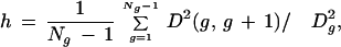where

is the average over each of the experimental conditions c of the square of the difference between the expression values v(g,c) and v(g + 1,c) of genes g and g + 1, and D is the expected value of D² when the expression values are drawn independently from a random distribution with zero mean and unit variance. It can be easily shown that D = 2. Thus, our heterogeneity measure is a positive number with a value that is zero if the gene expression were homogeneous (i.e., each gene in the class had the same gene expression profile), and with an average that is one when the gene expression values are random.

Figure 5A shows the true positive rate versus the heterogeneity measure for each of the 96 functional classes considered. There seems to be a linear relationship between the rate of TP and heterogeneity measure. As expected, the more homogeneous classes are learned with a higher rate of TP. Indeed the best learned class is the class of ribosomal proteins, which is the most homogeneous one (see Fig. 4A), and the heterogeneity measure of the worst learned classes is close to 1.

Figure 5.

(A) True-positive rate versus the heterogeneity measure (defined in the text) for all functional classes. (B) Heterogeneity measure versus the size of the class. The solid line is a linear fit to the data with correlations coefficient −0.37 and slope of −0.0001.

Heterogeneity and class size are, to some extent, independent factors that affect the learning rate of a class. To study systematically the relationship between heterogeneity and class size, the former is plotted versus the latter in Figure 5B. There seems to be a very faint trend for smaller classes to be more heterogeneous, whereas larger classes tend to be more homogeneous. However, except for extreme class size, the trend is hardly noticeable. A linear fit to the data of Figure 5B yields a very small correlation coefficient (−0.37), and an almost flat slope. Indeed, between classes of sizes five and 100, the size of the class hardly determines the heterogeneity of the class.

The Borges Effect: The Internal Structure of a Catalog Affects Its Learning Rate

We have discussed the influence of class size and heterogeneity in determining how well a class can be learned. In this section we shall see that the effect that the internal structure of the catalog of functional classes has on the performance of a machine-learning task is substantial. Concisely, one important reason why some classes cannot be learned is that they share members with other classes. When a nonnegligible amount of class members intersect with other classes and thus are both members of the class to be learned and the complementary set, machine-learning algorithms will face serious difficulties in distinguishing positive from negative examples.

Perhaps an illustration taken from a widely cited work of writer and philosopher Jorge Luis Borges (1964) will bring this point home, not without some humor. Referring to the inability of language to explain the universe, Borges describes an imaginary encyclopedia:

These ambiguities, redundances, and deficiencies recall those attributed by Dr. Franz Kuhn to a certain Chinese encyclopedia entitled Celestial Emporium of Benevolent Knowledge. On those remote pages it is written that animals are divided into (a) those that belong to the Emperor, (b) embalmed ones, (c) those that are trained, (d) suckling pigs, (e) mermaids, (f) fabulous ones, (g) stray dogs, (h) those that are included in this classification, (i) those that tremble as if they were mad, (j) innumerable ones, (k) those drawn with a very fine camel's hair brush, (l) others, (m) those that have just broken a flower vase, (n) those that resemble flies from a distance.

When trying to differentiate “stray dogs” from the rest of the animals, it is likely that some stray dogs will not be identified correctly: Some of them might indeed “resemble flies from a distance,” or “tremble as if they were mad.”

The inability of our machine-learning algorithm to perform without incurring in a great number of misclassifications is related to the fact that the classes in the MIPS catalog are not equivalence classes. Note that this is not a limitation of the design of the MIPS catalog, but rather an inherent property of biology, in which different biochemical processes interact. For example, the glyoxylate cycle “talks” with the TCA cycle and with the glycolysis process (see Fig. 1B). We believe that this phenomenon will tend to occur whenever we attempt to learn biological classes in a somewhat reductionistic way: When a biological process is isolated for a machine-learning task, the poor learning rate for this process responds to the fact that biology tends to work in a complex and highly interacting manner.

We wish to propose the term “Borges effect” to describe this inherent limitation of classification systems. The Borges effect can be quantified. We shall introduce two quantities to measure how intermingled the gene sets with the signatures that we are trying to learn are. Let C_i be the i-th out of N sets. Each of these sets is composed of genes that share given functional features (i.e., they participate in a specific biological process). The universe of genes to be considered is then U = C₁ ∪ C₂ ∪…∪ C_N. Genes could belong to two or more sets. For example, ORF YDL078C (gene name MDH3) belongs to the following sets: carbohydrate metabolism; lipid, fatty acid and sterol metabolism; other energy generation activities; and peroxisomal organization.

Given a set C, we can define its link number, denoted by L(C), as the number of sets with which C has a nonnull intersection. The link number L(C) ranges between 0 and N − 1 (the total number of sets excluding C). When the link number of a set is divided by the set size, the resulting quantity is a measure of the average number of sets that a member of C belongs to. We will call this quantity the link number per gene. We also define the sharing number of a set C, S(C), as the number of members of C that are members of other sets in the catalog; that is, S(C) = #(C ∩ (U − C)), where #(C) denotes the number of members, or cardinality, of set C. The relative sharing number s(C), ranging between zero and one, is defined as S(C) divided by the total number of members of C. The relative sharing number measures the proportion of a set that is shared by other members of the catalog. The sharing and link numbers for the functional catalog of MIPS are shown in Figure 6.

Figure 6.

(A) The relative sharing number as a function of class size. (B) Link number per gene for each class versus the class size #C (circles) and a straight line (dashed line) that shows the trend of the link number per gene to decrease as #(C)^−1/2 (notice the log-log scale). (C) The percentage of true positives versus the link number per gene. (D) The heterogeneity measure of a class in terms of its link number per gene.

Figure 6A shows the relative sharing number of each functional class as a function of class size. We can see that independent of size, almost every class shares almost all its members with other classes. The relative sharing number averaged over all classes is 0.93; that is, on average 93% of each class is shared. This observation helps to understand why overall, the functional MIPS catalog is learned with very low TP rates: For all of its classes, most of the genes belong to at least some other functional class.

In Figure 6B, we plot the link number per gene for each class versus the class size. When the class size increases, there are more opportunities for the class to intersect with other classes, and indeed the number of links L(C) increases. However, this increase is sublinear, and the link number per gene (defined as L(C)/#(C)) decreases with the class size #(C). This decrease appears to be proportional to #(C)^−1/2, as indicated in the dashed line of Figure 6B. The link number averaged over all the classes is 26: In average, each class overlaps with 26 other classes in the catalog. The average link number per gene is 0.9; that is, for each set in the catalog, each of its genes typically belongs in average to one other set.

Recall that the interpretation of the link number per gene of a class is the average number of other sets that a gene in said class belongs to. We should expect that a small link number per gene would result in higher rate of learning. This is the general trend shown in Figure 6C, in which we plotted the percentage of TP versus the link number per gene. All classes learned with a TP rate >40% had a link number per gene <0.6. All classes with a link number per gene greater than one were learned with a TP rate <25% (with the exception of a class that had a TP rate of 35).

It can be argued that there must be a relationship between the heterogeneity measure of a class and its link number per gene. If the link number per gene of a class is large, the class must accommodate the gene expression profiles of those classes that have nonnull intersection with itself, and therefore, it should exhibit a somehow large heterogeneity measure. In Figure 6D, we have plotted the heterogeneity measure of a class in terms of its link number per gene. There is a trend, albeit faint, showing that the heterogeneity shows a tendency to increase with the link number per gene.

Let us recapitulate the main observations made in this section. The Borges effect is one of the determining factors in the performance of a learning machine: Classes with a small link number per gene tend to be learned better. The Borges effect also provides an explanation for the better learning performance of larger classes: Larger classes exhibit smaller link numbers per gene, and therefore it should be expected that a learning process performs better on them. Finally, the Borges effect is related to the heterogeneity of a class: The more homogeneous classes tend to have smaller link number per gene and thus are learned better.

We have seen that the performance of our learning scheme is relatively poor, in the sense that ∼92% of the classes are learned with a rate of FN >40%. However, the results of this section indicate that the FNs and the FPs are not random: The class being learned is likely to recruit FPs from, and lose FNs to, the classes it is linked with. We had analyzed this effect in detail for the TCA cycle earlier. The results of this section provide evidence that such effect is likely to be more general.

Iterative Learning

We have seen that the FPs arising from learning a class C₀ can play a role in biological processes closely related to this class. If the Borges effect is at play, these FPs are likely to be genes belonging to other functional classes whose intersection with C₀ is nonnull. Taking this behavior into account, we propose an iterative learning procedure in which we augment the class C₀ with the FPs that arise from its learning, thus eventually creating a new class with better learning performance and that recapitulates the relationships of genes across functional classes and pathways.

The procedure works as follows. After a learning step, we add the newly produced FPs to the original class C₀ to form an extended class C₁. These new added members will serve as examples to facilitate the learning of the classes intersecting with the original class. We next attempt to learn C₁, thus creating a new set of FPs, which are added to C₁ to form C₂ and so on. On iterating this process, two scenarios can arise: (1) The iterations converge (i.e., no new FPs are found after a number of steps) to an extended class of genes that participate in biological processes related to the original class C₀, or (2) the basin of attraction for the augmented class keeps growing until it comprises most of the genes in the whole data set.

We tested our iterative procedure using the TCA cycle as the original class C₀. In the first stage of the iteration, we trained the MLP to recognize members of C₀, and we identified the FPs using the threefold cross-validation scheme, with a threshold of τ = 0.8. After adding the FP genes to C₀ to create the class C₁, we trained the MLP again, and so on. Recall that the cross-validation scheme randomly partitions classes into three subsets. Thus, different replicas of the cross-validation, even at the same iteration number, may yield a different number of FPs. In this way, we get an average number of FPs and a standard deviation at each iteration step. An iteration that yields zero FPs would be a clear sign that the process is convergent. However, it should be noted that even then, the following iteration could still give rise to a nonzero number of FPs, owing to the randomness of the subsequent partitions.

Setting the threshold τ, which determines whether a gene is a FP or not, is very important for an efficient performance of the iterative process. If τ is too low, the iteration might not converge at all, and the augmented class would grow to include all the genes in the data set. On the other hand, if the threshold is too stringent, the iteration might stop after the first step. Park et al. (1998) reported a similar problem in using an intermediate sequence search procedure to increase the number of sequences detected by similarity. We ran the learning procedure with different τ values to study this effect. We chose the optimal threshold as the less stringent value for which the iteration still converges. This gave us τ = 0.8.

The solid line with circles in Figure 7A shows the results of the iteration process on the TCA class. The dotted line with diamonds shows the results for a database of gene expression with the same dimensions, but with the 79 components of the expression vector randomized. The curves show the average number of FPs at each iteration with their respective error bars. The learning procedure consistently produced substantially fewer FPs for the actual data.

Figure 7.

(A) The number of false positives as a function of the iteration number in iterative learning process of the TCA class (circles and solid line) and of a randomized control (diamonds and dashed curve). (B) Same as in A, but for false negatives.

There is a sustained trend of decreasing FPs in the TCA data as the number of iterations increases (especially in the first four iterations). This trend is much less obvious in the randomized data, in which at some iteration the average number of FPs seems to increase strongly (iterations 2, 8, and 9). Figure 7B shows the number of new FNs as a function of the iterations, which stabilizes at ∼10 for the TCA data; note that because the class size increases during the process, the relative number of FNs actually decreases. On the other hand, the number of FNs for the randomized data shows an increasing trend, reaching ∼30 FNs at the 10th iteration (about three times higher than for the actual data). That is, the randomized data shows a much larger FN rate, indicating the nonrandom nature of the FNs obtained for the real data.

For the actual data, each of the five replicas reached a value of zero FPs at some iteration. (No individual replica reached zero FP for the randomized data.) One particular replica reached zero FP at iteration 4. Figure 8, which pertains to this replica, is a representation of the classes to which the successive FPs belonged to, and a clear example of the Borges effect. At the center of Figure 8 is the TCA cycle class (comprising 17 genes). The other classes that are represented in the innermost circle share some of the TCA cycle members. A solid line linking two classes indicates that the two classes share at least one member. Because the link number for the TCA class is seven, the first circle (iteration 0) contains seven classes. At the first iteration, we obtained 14 FPs. The new classes to which these FPs belong (and that were not plotted in the innermost circle) are listed in the second circle. It should be noticed that some of the new FPs belong to more than one class. The second iteration yielded five FPs, which added four new classes (shown in the third circle). Two of these classes were not linked with any of the previous classes, but these two classes actually stem from the same gene (YGL200C). The third iteration yielded four new genes, only one of which did not belong to previously encountered classes and which contributed the two new classes appearing in the outer circle. The fourth iteration yielded no FPs at all, and we stopped our analysis there.

Figure 8.

Schematic representation of the classes to which the successive FPs belonged to in the process of iterative learning. Each circle represents a step in the iterative learning process. The TCA cycle genes (at the center) intersect the classes that are represented in the innermost circle. A solid line connecting two classes indicates that the two classes share at least one member. If a new iteration yields one or more false positives, the corresponding circle will contain all the functional classes that these false positives belong to (except for the classes already represented at inner circles), linked by lines to all the classes in the inner circles with which they have nonnull intersection.

Of the 23 FPs discovered in the iterations described above, only two did not belong to the web of class intersections related to the TCA cycle in the center. The picture emerges that the discovered FPs are functionally related to the TCA cycle, rather than being the product of random errors in the learning process. Figure 8, constructed merely on the basis of our machine-learning procedure, looks like a coarse grained roadmap of the cellular processes associated with the energy metabolism.

DISCUSSION

In this paper, we tested the ability of the MLP machine-learning technique to extract the signature of yeast functional classes from gene expression data over 79 experimental conditions. The antecedent of this study is the work of Brown et al. (2000), who used several machine-learning algorithms, concluding that SVM performed the best in terms of a score based on FP and FN. We applied MLP for the first time to the same data to compare our results to those of Brown et al. Both SVMs and MLP yielded a similar number of FNs. However, the MLP-based scheme produced a systematically bigger number of FPs. Subsequently, we explored the biological nature of the FPs arising from our algorithms for one functional class, the TCA cycle. The conclusion was that machine-learning FPs were not necessarily biological FPs. In other words, most of the FPs had a biological function associated with the TCA cycle. The FPs were in many cases enzymes interacting with metabolites that are also channeled through the TCA cycle. We showed this in Figure 1B, in which three members of the glyoxylate cycle (which allows the synthesis of carbohydrates from lipids), CIT2, MLS1, and MDH2, are recruited as FPs by our learning scheme. Thus, we can hardly say that the MLP is unable to “learn” the classes compared with SVMs. Indeed, it uncovers the underlying biology in a very surprising way.

Provided that the last premise is accepted, it makes sense to undertake the task of testing how “learnable” the rest of the functional classes cataloged in MIPS are. To the best of our knowledge, this systematic study has not been reported before. Our results are a priori unexpected: Most of the classes are nonlearnable, if by learnable we mean having a reasonably low FN rate. Indeed, 92% of the classes were learned with a FN rate worse than 60%. We explored the reasons for this poor performance. Assuming that the microarray experiments contain a sufficiently high signal to noise ratio, we identified three factors determining the learning performance. The first one is the size of the functional classes: Classes that are of small size learned more poorly than did classes of larger size. A second factor identified was the heterogeneity of classes. We defined a measure of heterogeneity and showed that learning performance degrades as this heterogeneity measure increases. The third factor stems from the fact that the functional classes in the MIPS catalog are not equivalence classes. In fact, transitivity is not always met: If genes A and B belong to the same class and genes B and C belong to the same class, then A and C do not necessarily belong to the same class. This complicates the learning process substantially. In effect, when we try to learn the signature for the class to which gene A belongs, we will also learn the signature of gene B; thus, genes with a gene expression profile similar to that of B from the class in which C belongs may be erroneously annotated as belonging to the class of A (false positives). Alternatively, the class of C may recruit gene B, thus creating a false negative. These false positives and false negatives are recruited through genes such as B, which act as links between the class of A and the class of C. We have called this the Borges effect. We quantified the Borges effect with two indices: the link number per gene and the relative sharing number. For equivalence classes these indices are zero, and the larger these quantities are, the more intermingled the classes will be. We conjecture that for catalogs in which any of these indices takes large values, any learning machine will perform poorly (the average relative sharing number was 0.92 in the classification system we used). We believe that this effect warrants more research.

In the light of the Borges effect, we can rethink why the machine-learning errors are not necessarily biological errors: When learning a class, it is very likely that the FPs found were from a set that intersects with the original class to be learned. But if these classes intersect, it means that they are functionally related. Thinking along these lines, we developed an iterative learning scheme, in which at any given iteration, the FPs at one learning step are added to the original class to be learned in the next iteration. The augmented classes that appear at successive iterations will thus be functionally related to the original class at iteration 0. We implemented this iterative scheme using the TCA cycle as the starting class. The results, shown in Figure 8, look like a coarse grain reconstruction of the processes functionally related to the TCA pathway. Thus, it seems that this iterative scheme could be used as a tool to unravel coarse features of complex and interacting systems. Of course, much more work is needed in this direction.

In summary, we have studied the limitations in learning functional classes from DNA microarray data, and we concluded that those limitations are strongly related to the structure of the catalog of biological functions, to the heterogeneity of the expression profile within the classes, and to the class size. Our results and inferences, however, are derived from a particular set of mRNA expression data. It may be possible that different data sets (e.g. Rosetta's data series corresponding to 300 diverse mutations and chemical treatments, see http://www.rii.com/tech/pubs/cell_hughes.htm) or subsets of the experimental conditions used in the present paper may yield a different learning performance.

We also made the point that machine-learning false positives are not necessarily biological false positives. In that respect, we believe that our analysis of the TCA cycle constitutes proof of principle of our contention. (The reason why we used the TCA cycle is that the wealth of information available for this metabolic pathway helped us in the interpretation of the results.) Our conclusions, however, were not tested in other functional classes.

Our work opens a number of interesting questions. Do our results generalize to other catalogs such as biological pathways and complexes? Are there classes for which learning statistics change significantly as a function of the expression data set? Does the iterative algorithm connect a different set of neighbor interactions when the learning is performed on different data sets? Do the results found for the TCA cycle generalize to other classes? These important questions will be addressed in future studies.

METHODS

DNA Microarray Data and Classes

Gene expression profiles of 2467 annotated genes from S. cerevisiae in 79 different DNA-array experiments, including the time series along the cell cycle (Eisen et al. 1998), were analyzed. The classes used for the training process of the SNN were taken from the Yeast Genome Database at the MIPS, in particular, the 99 functional classes corresponding to the second level of the MIPS functional catalog (http://mips.gsf.de/proj/yeast/catalogues/funcat, version of November 8, 2001). Of the MIPS catalog, only classes containing at least three genes present in Eisen et al.'s (1998) data set were used, which made the number of trained classes 96, slightly smaller than the actual number of cataloged classes.

Back-Propagation Neural Networks

The SNNS package program (http://www.ra.informatik.uni-tuebingen.de/SNNS/) was used to implement the neural network, in this case a MLP. We used a perceptron with standard back-propagation (Rumelhart et al. 1986) as learning function and updated by topological order. To introduce nonlinearity into the network, the logistic activation function was used. The network has 79 input neurons corresponding to the 79 DNA array experimental conditions. There is no theory that relates the number of hidden layers necessary to properly identify classes in a given problem, but one hidden layer with an appropriate number of hidden units suffices the “universal approximation” property (Bishop 1995). MLPs with more layers are more prone to over-fit the problem and fail in learning the general features of the class. Similar arguments can be used for the choice of the number of units in the hidden layer. There are several rules of thumb, and a general agreement is that this number must be between the number of input and output units. A good choice for the number of hidden units seems to be a value around the square root of the number of units in the previous layer (the input layer in this case; Blum 1992). We have explored the performance of the MLP using one hidden layer with five, eight, and 20 hidden units (data not shown). The results between these different architectures were very consistent. We opted to use eight hidden units, a choice that yielded a good compromise between generalization and error. The MLP used here, then, has one hidden layer with eight units connected to any of the 79 input neurons and one output unit, for the case of learning one class at a time. In the case of learning simultaneous classes, the network topology includes as many output units as classes to be learned.

The neural network is trained with a training set, which contains examples corresponding to each of the possible groups to be learned. When the number of examples corresponding to different groups in the training sets shows a serious asymmetry in sizes, the examples corresponding to the class smaller in size are presented more times to the network to compensate the otherwise unbalanced training set.

Three-Way Cross-Validation

The performance of the learning process was checked using a three-way cross-validation scheme. Both the set C to be learned and its complement U − C (where U is the set of all genes under consideration) were randomly divided into three groups. The MLP was trained with two of these groups (the training set) and the remaining group (the test set) was used to test the network. Each gene belonging to C in the test set can either be predicted to be in set C (in which case it will be deemed to be a true positive, or TP), or in set U − C (in which case it will be deemed to be a false negative, or FN). Alternatively, each gene belonging to U − C in the test set can either be predicted to be in set C (in which case it will be deemed to be a false positive, or FP), or in set U − C (in which case it will be deemed to be a true negative, or TN). The procedure was repeated two more times for the other two possible combinations of groups. The performance of the learning scheme, as measured by the total number of FP, FN, TP, and TN is obtained as the sum of the performances under the three combinations of groups. In this way, the sum of the number of TP and FN is equal to the number of members in the original set C, and the sum of the number of TN and FP is equal to the number of members in the set U − C. It should be noticed that, because of the random nature of the partition of the sets, different runs of this three-way cross-validation scheme could yield different numbers of TP and FN, even though the sum is always equal to the number of members in the class being learned.

Hierarchical Clustering and Eisen Plots

The hierarchical clustering algorithm used to generate the dendrograms of Figure 4 is based on the average-linkage method (Hartigan 1975; Eisen et al. 1998). The expression value of each gene is normalized to have zero mean and unit standard deviation across the 79 experimental conditions. The distance between two individual samples is calculated by euclidean distance with the normalized expression values. Both the genes and the conditions are organized according to the hierarchical clustering method. The gene expression is graphically represented using color-coded matrices (the so-called Eisen plots; Eisen et al. 1998). Columns represent individual experimental conditions, and rows represent individual genes present in the class. To generate a pseudo-color map the normalized gene expression value v is used. The pseudo-color map represents v = 0 as black, v > 0 as progressively brighter hues of red, and v < 0 as progressively brighter levels of green. v > 2 and v < −2 correspond to complete saturation of the red and the green, respectively. The resulting pseudo-color map associates the same colors to measurements that are off by the same number of standard deviations from their average.

WEB SITE REFERENCES

http://www.ra.informatik.uni-tuebingen.de/SNNS; SNNS package program.

http://www.cse.ucsc.edu/research/compbio/genex; from which the statistics for the SVMs were extracted.

http://www.rii.com/tech/pubs/cell_hughes.htm; Rosetta's data series corresponding to 300 diverse mutations and chemical treatments.

http://mips.gsf.de/proj/yeast/catalogues/funcat; 99 functional classes corresponding to the second level of the MIPS functional catalog, version of November 8, 2001.

REFERENCES

- Alizadeh AA, Eisen MB, Davis RE, Ma C, Lossos IS, Rosenwald A, Boldrick JC, Sabet H, Tran T, Yu X, et al. Distinct types of diffuse large B-cell lymphoma identified by gene expression profiling. Nature. 2000;403:503–511. doi: 10.1038/35000501. [DOI] [PubMed] [Google Scholar]
- Alon U, Barkai N, Notterman DA, Gish K, Ybarra S, Mack D, Levine AJ. Broad patterns of gene expression revealed by clustering analysis of tumor and normal colon tissues probed by oligonucleotide arrays. Proc Natl Acad Sci. 1999;96:6745–6750. doi: 10.1073/pnas.96.12.6745. [DOI] [PMC free article] [PubMed] [Google Scholar]
- Alter O, Brown PA, Botsein D. Singular value decomposition for genome-wide expression data processing and modelling. Proc Natl Acad Sci. 2000;97:10101–10106. doi: 10.1073/pnas.97.18.10101. [DOI] [PMC free article] [PubMed] [Google Scholar]
- Arfin SM, Long AD, Ito ET, Tolleri L, Riehle MM, Paeglei ES, Hatfield GW. Global gene expression profiling in Escherichia coli K12. J Biol Chem. 2000;38:29672–29682. doi: 10.1074/jbc.M002247200. [DOI] [PubMed] [Google Scholar]
- Ben-Dor A, Shamir R, Yakhini Z. Clustering gene expression patterns. J Comput Biol. 1999;6:281–297. doi: 10.1089/106652799318274. [DOI] [PubMed] [Google Scholar]
- Bishop CM. Neural networks for pattern recognition. Oxford: Clarendon Press; 1995. [Google Scholar]
- Blum A. Neural networks in C++. New York: Wiley; 1992. [Google Scholar]
- Borges JL. Other inquisitions. Austin, TX: University of Texas Press; 1964. The analytical language of John Wilkins. [Google Scholar]
- Brown MPS, Grundy WN, Lin D, Cristianni N, Sugnet CW, Furey TS, Ares M, Haussler D. Knowledge-based analysis of microarray gene expression data by using support vector machines. Proc Natl Acad Sci. 2000;97:262–267. doi: 10.1073/pnas.97.1.262. [DOI] [PMC free article] [PubMed] [Google Scholar]
- Califano A, Stolovitzky G, Tu Y. Analysis of gene expression microarrays for phenotype classification. Proc Int Conf Intell Syst Mol Biol. 2000;8:75–85. [PubMed] [Google Scholar]
- Eisen MB, Spellman PT, Brown PO, Botstein D. Cluster analysis and display of genome-wide expression patterns. Proc Natl Acad Sci. 1998;95:14863–14868. doi: 10.1073/pnas.95.25.14863. [DOI] [PMC free article] [PubMed] [Google Scholar]
- Furey TS, Cristianini N, Duffly N, Bednarski DW, Schummer M, Haussler D. Support vector machine classification and validation of cancer tissue samples using microarray expression data. Bioinformatics. 2000;16:906–914. doi: 10.1093/bioinformatics/16.10.906. [DOI] [PubMed] [Google Scholar]
- Golub TR, Slomin DK, Tamayo P, Huarol C, Gaasenbeek M, Mesirov JP, Coller H, Loh ML, Downing JR, Caligiuri MA. Molecular classification of cancer: Class discovery and class prediction by gene expression monitoring. Science. 1999;286:531–537. doi: 10.1126/science.286.5439.531. [DOI] [PubMed] [Google Scholar]
- Hartigan JA. Clustering algorithms. New York: Wiley; 1975. [Google Scholar]
- Herrero J, Valencia A, Dopazo J. A hierarchical unsupervised growing neural network for clustering gene expression patterns. Bioinformatics. 2001;17:126–136. doi: 10.1093/bioinformatics/17.2.126. [DOI] [PubMed] [Google Scholar]
- Heyer LJ, Kruglyak S, Yooseph S. Exploring expression data: Identification and analysis of coexpressed genes. Genome Res. 1999;9:1106–1115. doi: 10.1101/gr.9.11.1106. [DOI] [PMC free article] [PubMed] [Google Scholar]
- Hill AA, Hunter CP, Tsung BT, Tucker-Kellog G, Broiwn EL. Genomic analysis of gene expression in C. elegans. Science. 2000;290:809–812. doi: 10.1126/science.290.5492.809. [DOI] [PubMed] [Google Scholar]
- Khan J, Wei JS, Ringnér M, Saal LH, Ladanyi M, Westermann F, Berthold F, Schwab M, Antonescu CR, Peterson C, et al. Classification and diagnostic prediction of cancers using gene expression profiling and artificial neural networks. Nature Med. 2001;7:673–679. doi: 10.1038/89044. [DOI] [PMC free article] [PubMed] [Google Scholar]
- Kohonen T. Self-organizing maps. Berlin, Germany: Springer-Verlag; 1997. [Google Scholar]
- Mewes HW, Frishman D, Gruber C, Geier B, Haase D, Kaps A, Lemcke K, Mannhaupt G, Pfeiffer F, Schuller C, et al. MIPS: A database for genomes and protein sequences. Nucleic Acids Res. 2000;28:37–40. doi: 10.1093/nar/28.1.37. [DOI] [PMC free article] [PubMed] [Google Scholar]
- Park J, Karplus K, Barret C, Hughey R, Haussler D, Hubberd T, Chothia C. Sequence comparisons using multiple sequences detect three times as many remote homologues as pairwise methods. J Mol Biol. 1998;284:1201–1210. doi: 10.1006/jmbi.1998.2221. [DOI] [PubMed] [Google Scholar]
- Perou CM, Jeffrey SS, van de Rijn M, Rees CA, Eisen MB, Ross DT, Pergamenschikov A, Williams CF, Zhu SX, Lee JCF, et al. Distinctive gene expression patterns in human mammary epithelial cells and breast cancers. Proc Natl Acad Sci. 1999;96:9112–9217. doi: 10.1073/pnas.96.16.9212. [DOI] [PMC free article] [PubMed] [Google Scholar]
- Rosenblatt F. The perceptron: A probabilistic model for information storage in the brain. Psych Rev. 1958;65:386–407. doi: 10.1037/h0042519. [DOI] [PubMed] [Google Scholar]
- Rumelhart DE, Hinton GE, Williams RJ. Learning internal representations by error propagation. In: Rumelhart DE, et al., editors. Parallel distributed processing. Vol. 1. Cambridge, MA: MIT Press; 1986. pp. 319–362. [Google Scholar]
- Schena M, Shalon D, Davis RW, Brown PO. Quantitative monitoring of gene expression patterns with a DNA microarray. Science. 1995;201:467–470. doi: 10.1126/science.270.5235.467. [DOI] [PubMed] [Google Scholar]
- Shalon D, Smith SJ, Brown PO. A DNA microarray system for analyzing complex DNA samples using two-color fluorescent probe hybridization. Genome Res. 1996;6:639–645. doi: 10.1101/gr.6.7.639. [DOI] [PubMed] [Google Scholar]
- Sneath PHA, Sokal RR. Numerical taxonomy. San Francisco, CA: Freeman; 1973. [Google Scholar]
- Tamayo P, Slonim D, Mesirov J, Zhu Q, Kitareewan S, Dmitrovsky E, Lander ES, Golub TR. Interpreting patterns of gene expression with self-organizing maps: Methods and application to hematopoietic differentiation. Proc Natl Acad Sci. 1999;96:2907–2912. doi: 10.1073/pnas.96.6.2907. [DOI] [PMC free article] [PubMed] [Google Scholar]
- Tavazoie S, Hughes JD, Campbell MJ, Church GM. Systematic determination of a genetic network architecture. Nat Genet. 1999;22:281–285. doi: 10.1038/10343. [DOI] [PubMed] [Google Scholar]
- Törönen P, Kolehmainen M, Wong G, Castrén E. Analysis of gene expression data using self-organizing maps. FEBS Lett. 1999;451:142–146. doi: 10.1016/s0014-5793(99)00524-4. [DOI] [PubMed] [Google Scholar]
- Vapnik V. Statistical learning theory. New York: Wiley; 1998. [Google Scholar]
- Zhang L, Zhou W, Velculescu VE, Kern SE, Hruban RH, Hamilton SR, Volgestein B, Kinzler KW. Gene expression profiles in normal and cancer cells. Science. 1997;276:1268–1272. doi: 10.1126/science.276.5316.1268. [DOI] [PubMed] [Google Scholar]