An adaptation of the LMS method to determine expression variations in profiling data

Abstract

One of the major issues in expression profiling analysis still is to outline proper thresholds to determine differential expression, while avoiding false positives. The problem being that the variance is inversely proportional to the log of signal intensities. Aiming to solve this issue, we describe a model, expression variation (EV), based on the LMS method, which allows data normalization and to construct confidence bands of gene expression, fitting cubic spline curves to the Box–Cox transformation. The confidence bands, fitted to the actual variance of the data, include the genes devoid of significant variation, and allow, based on the confidence bandwidth, to calculate EVs. Each outlier is positioned according to the dispersion space (DS) and a P-value is statistically calculated to determine EV. This model results in variance stabilization. Using two Affymetrix-generated datasets, the sets of differentially expressed genes selected using EV and other classical methods were compared. The analysis suggests that EV is more robust on variance stabilization and on selecting differential expression from both rare and strongly expressed genes.

INTRODUCTION

In the context of the Human Genome Project, new technologies have emerged allowing the simultaneous analysis of a large number of genes in a single experiment. The so-called DNA micro-arrays or DNA chips constitute a prominent example. The goal of many of these experiments is to identify differentially expressed genes in cultured cells or tissue samples under different physiological or pathological conditions. RNA expression differences are often determined by calculating the ratios of hybridization signals between a test and a reference sample. One of the characteristics of expression profiling is that, in a typical experiment, thousands of genes are analyzed on a small number of experimental conditions. However, it has proved challenging to identify genuine expression differences while simultaneously avoiding false positives.

Since the variance is inversely proportional to the log of the signal intensities, and the signal intensities range from 1 (rare) to 10⁵ (strongly expressed genes), although the noise is the same for each gene analyzed on a given array, the noise has more impact on the large majority of weakly expressed genes than on the small fraction of strongly expressed genes.

The variation on these experiments has many components, including the variability of the biological samples, labeling conditions, array specificity, reading efficiency for each spot, etc. These variations can be categorized as systematic variation, which can easily be corrected for, and are referred to as calibration and normalization as discussed by Balding et al. (1). Other variations, however, are random, and may be accounted for through error models. Several models have been used with more or less success, to correct for random variation, including a model based on the generalized logarithm (glog) (2), which has been applied by a number of authors to stabilize the variance (3–5). Alternative approaches have been proposed such as noise filtering look up tables (LUT) (6), which uses a scoring system in which a given context will provide predictive values for reproducibility in fold change (FC) results (7).

Here, we adapt the LMS approach, originally described by Cole and Green (8), to model gene expression profiling data. The authors initially used this approach for growth charts of children. LMS allows to construct smoothing reference centile curves, which fit cubic spline curves to the Box–Cox transformation. This transformation leads to normalization of the variance and thus defines standard intervals for significant expression differences. Using this transformation, a confidence band adjusted to the actual distribution of the data is defined, which identifies the set of genes devoid of expression differences. The confidence band was determined after applying a spline fit, determining the median axis of the plot and the spline curves defining the lower and upper limits of the dispersion space (DS). Expression variation (EV) measurements are then based on the size of this DS. Here, we present the application of this method, and comparisons with other strategies, on a dataset generated using the Affymetrix platform.

MATERIALS AND METHODS

The LMS method

The essential background of the LMS approach described by Cole and Green (8) is summarized below. The usual assumptions for data analysis are the standard assumptions of the linear model, i.e. the existence of additive effects, the constancy of variance, the normality of the variables and the independence of observations. If these assumptions are not satisfied, two alternatives are possible: either to devise a new analysis that meets these assumptions, or to transform the data in order to meet these assumptions. It is almost always easier to use a satisfactory transformation than to develop a new method of analysis. Tukey (9) suggested a family of transformations with an unknown power parameter λ and Box and Cox (10) modified it. The ‘classical’ Box–Cox power transformation of the dependent variable is a useful method to alleviate heteroscedasticity for dependent variables with an unknown distribution.

The LMS method (11) models the variable y as a semiparametric regression function of the dependent variable x, so that the distribution of y changes smoothly when plotted against x. The distribution is summarized by three spline curves: the Box–Cox power that converts y to normality (L), the mean (M) and the coefficient of variation (S). The main application of this method is to generate reference centile curves. The transformed observations are independent and normally distributed with constant variance. The Box–Cox transformation is defined as

1

where y is the response variable and λ is the transformation parameter.

For λ = 0, the natural log of the data is taken instead of using the above formula, since the ratio is undefined.

Based on this family of transformations, the LMS method described by Cole and Green (8,11) assumes that it is appropriate to consider the transformed variable

2

and

where μ is the median of y. This transformation maps the median of y to = 0, and it is continuous at λ = 0. Denoting the standard deviation of by σ, the variable

3

and

is assumed to have a standard normal distribution.

Assuming now that the distribution of y varies with covariate x, and that λ, μ and σ at x are read off the smooth curves L(x) (Box–Cox power), M(x) (median) and S(x) (coefficient of variation). The initials of these parameters give the name of the LMS method. So the formula

4

and

converts the measurement y to its normal equivalent deviate z.

Cole and Green (8) pointed in the discussion of their article that for n independent observations y_i at corresponding values x_i, the log-likelihood function derived from (4) is proportional to

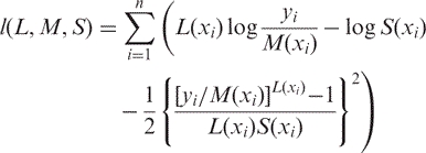5

and the curves L(x), M(x) and S(x) are estimated by maximizing the penalized likelihood

6

The α_L, α_M and α_S values are usually called the smoothing parameters and can be regarded as the tuning parameters that control the trade-off between goodness of fit of the data and smoothness. They are used for each of the L, M and S curves, where larger values correspond to stronger smoothing.

The three L, M and S curves can be estimated with spline functions. This form of penalty leads to natural cubic splines with knots at each distinct value of x. Basic references for spline descriptions can be found in Wegman (12) and Nürnberger (13), although the essential background is described here for self-completeness of the article.

A cubic spline is a piecewise cubic polynomial such that the function, its derivative and its second derivative, are continuous at the interpolation nodes. The natural cubic spline has zero second derivative at the endpoints. It is the smoothest of all possible interpolating curves, since it minimizes the integral of the square of the second derivative. A knot is a point in the domain space of a function where pieces of a fitted surface join.

These parameters correspond to the equivalent degrees of freedom (edf) parameters. edfL, edfM and edfS, which specify edf for the L, M and S curves, respectively. The strategy to maximize the penalized likelihood function is to optimize the M curve edf, by increasing and/or decreasing the edf by 1 until the change in the penalized log likelihood is small (this depends on the sample size, but a change of less than two units is not significant—for large samples a bigger change is needed). This interactive procedure is stopped when the convergence in the likelihood maximization is obtained. Once the M curve is fitted, the process is repeated for the S curve. In many situations a constant value (i.e. 1 edf) is sufficient, and this should be tried first. Three edfs should then be tested, rather than two, which force a linear trend on the S curve and can lead to irrelevant values at the extremes of the range. Higher edf values may be suitable for large and/or complex datasets. Finally the L curve is fitted, in a similar way to S curve fitting. Cole and Green (8) modified the original Fortran program written to automatically fit the model. Parameter smoothing was done using LMS, a R package (http://www.biostat.harvard.edu/~carey/vcwww4.html) or the COLELMS Stat module (http://ideas.repec.org/c/boc/bocode/s360702.html). Once the L, M and S curves are estimated, any required centile curve can be derived from them.

The measurement centile is given by

7

where α defines the lower tail area of the centile and z_α is the normal equivalent deviate of size α. Hence C_α/2 and C_1−α/2 define a confidence bandwidth for the regression curve. In the next section, this confidence bandwidth will be referred to as DS.

Definition of the dispersion space

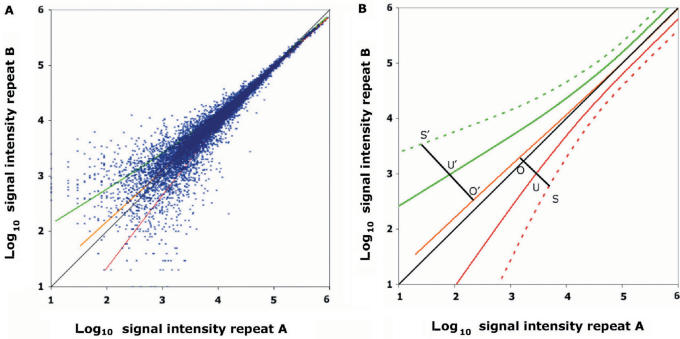
Maintaining the notation, x_i and y_i denote the expression of the ith gene in two experimental conditions. The confidence band defines the set of genes with constant expression or non-significant variation Equation [7]. The width of the confidence band, which will be referred to as DS, is dependent on the smoothing parameter α and can be adjusted if needed. Since the transformed z values have a standard normal distribution, the α value can be interpreted from a statistical point of view and DS(α) can be considered as a confidence bandwidth of level α. Therefore, α was set to α = 0.317, this defines splines for the DS that correspond to one standard deviation and include 68.3% of the spots (x_i, y_i value pairs) (Figure 1)A. Thus, each spot located outside the DS can be associated to a P-value (fractile of the normal distribution), which will define its deviation from normality and provide statistical support for the identification of differential expression (14,15).

Figure 1.

Gene expression scatter plot of Affymetrix oligo-array data and EV unit. (A) Dataset generated with Affymetrix chips. Hybridization, washes, antibody amplification and staining were performed using the Affymetrix fluidics station and scanner following the manufacturer's instructions. Data was log₁₀ scaled; scatter plots show uneven variance resulting in increased dispersion at low expression levels. Note that the first diagonal (black) and the median axis (yellow) do not overlap. Shown on the plot Median and confidence interval curves corresponding to parameter setting of α = 0.317 (green upper limit, red lower limit) are also shown on the plot. (B) DS (α = 0.317, green and red plain curves) and iso-variation representing expression variation EVα(X) = 2 (green and red dotted curves) correspond to the confidence limits defined with a P-value = 0.05. For each spot S, its orthogonal projection to the median O was determined and the distance between O and U d(O,U) (intersection of the segments O,U and the curve of the DS) measured. For each spot located along the O, S line, the value d(O,U) represents the unit of expression. Expression variation Evα(S) thus corresponds to the d(O,S)/d(O,U) ratio. |EV_α(S)| = 1 defines the baseline for genes presenting no EV. The plus sign was applied to values exceeding the upper spline limit and the minus sign to values below the lower spline limit.

Cells and RNA preparation culture conditions and reagents

B6.1 cell (16) is a mouse cytotoxic T cell clone requiring exogenous IL2 for growth. Cells were cultured in Iscove's modified Dulbecco's medium (IMDM) containing 10% heat-inactivated fetal calf serum, 10 mM Hepes pH 7.0, 0.05 mM β-mercaptoethanol, 2 mM glutamine and saturating concentrations of mouse rIL2 [1% X63mIL2 supernatant; (17)]. Cytoplasmic RNA from B6.1 cells exponentially growing in the presence of IL2, or a few hours after IL2 withdrawal was prepared using the NP40 method as described (18). After electrophoresis through denaturing 1.2% formaldehyde-agarose gels, RNA samples were transferred to nylon membranes (GeneScreen, NEN, Boston, MA) and rRNA distribution visualized by methylene blue staining (19).

Affymetrix GeneChip probe array hybridization

For cRNA synthesis, 10 µg of RNA from B6.1 cells, grown under different conditions, was used as a template for double-stranded cDNA synthesis using the Superscript Choice System (Invitrogen) and a T₇-(dT)₂₄ primer according to the Affymetrix protocol. After purification, double-stranded cDNAs were used as a template for in vitro T₇ transcription using the Bioarray high-yield transcript labeling kit (Enzo, Farmingdale, NY). Yields of cRNA synthesis (∼60 µg), were highly similar between different samples as monitored by spectrophotometry. Quality of in vitro transcribed cRNA was monitored with the BioAnalyzer Chip (Agilent Technologies, Palo Alto, CA), following the manufacturer's protocol.

Twenty-two micrograms of each cRNA population were fragmented. First, 5 µg was used to check the quality of the target on the Te3 test chips. Subsequently, 15 µg was used for hybridization of murine genome GeneChip probe arrays U74Av2 (both from Affymetrix, Santa Clara, CA). Hybridization, washes, antibody amplification and staining were performed following the manufacturer's instructions in an Affymetrix fluidics station and scanner. Analysis of the raw data was performed using Affymetrix Suite Software (MAS5) and NetAffx, VSN (5), or the EV method described here. The dataset is available as an Excel file at http://jasanz2.cib.csic.es/B61Database.xls

Affymetrix Latin square data for expression algorithm assessment

The data, freely available from Affymetrix, comes from the hybridization of 42 human genome U133 chips with three technical replicates of 14 separate hybridizations of 42 spiked transcripts in a complex human background at concentrations ranging from 0.125 to 512 pM. Thirty of the spikes are isolated from a human cell line, four spikes are bacterial controls and eight spikes are artificially engineered sequences believed to be unique in the human genome. The data is available at http://www.affymetrix.com/support/technical/sample_data/datasets.affx

RESULTS

Determining EVs

First of all, the DS comprising the invariant genes was defined, EV of outlier genes was subsequently assessed. This was done by measuring the distance d(O,S) between each spot ‘S’ and its orthogonal projection to the median ‘O’ (Figure 1). The distance d(O,U) between ‘O’ to the intersection between the segment [OS] and the DS curve was also measured, and EV of spot ‘S’ was defined as the ratio of these two distances: Ev_α(S) = d(O,S)/d(O,U). Therefore, Ev_α(S) represents the normalized value of the expression level. |Ev_α(S)| = 1 defines the baseline for genes presenting no EV. The plus sign was applied to values exceeding the upper spline limit and the minus sign to values below the lower spline limit (Figure 1B).

Threshold for EV

We applied this approach to a dataset obtained by expression profiling of the mouse B6.1 CTL cell line on 12K mouse Affymetrix MG-U74Av2 chips. As shown in Figure 1A, the plot of the data resulted in a comet shape, typical for expression profiling data, and the first diagonal did not overlap the median axis. As described above, each spot outside the DS is associated with a P-value.

Different settings will adjust the stringency applied to the selection of differentially expressed genes (different P-values). Since published data commonly show that the fraction of genes differentially expressed on subgenome-wide arrays range from 0.1 to 5% of the genes, depending on the nature of the array and the biological model studied (14,15), two commonly used P-values, namely 0.05 and 0.01, were utilized to determine the number of differentially expressed genes.

Assessing variance stabilization

First, it was verified that EV stabilized the variance, and then we compared the variance stabilization obtained with EV with other methods also known to stabilize variance, such as VSN, a method specifically devised to stabilize variance of expression array data (5). VSN defines a statistical model for gene expression profiling data based on an arcsinh transformation. It comprises data calibration, quantification of differential expression as well as of measurement error (http://www.dkfz.de/abt0840/whuber; R project and bioconductor library, at http://www.r-project.org/).

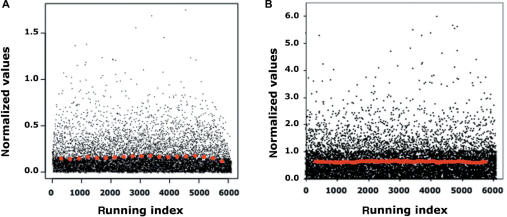
The VSN and EV approaches were applied in parallel to a previously studied Affymetrix dataset (20). It appears that both the EV and VSN transformations resulted in variance normalization (see Figure 2). EV-treated data showed a median for the standard deviation of 3.16%, with a range of absolute values of 5.98, whereas for VSN-transformed data the median for the standard deviation was of 3.25% and the range of absolute values of 1.75. Since for a 3-fold wider range of absolute data of EV as compared to VSN (5.98 versus 1.75), we have a similar median for the standard deviation, this can be interpreted as a 3-fold more robust variance stabilization of EV as compared to VSN. The same dataset was analyzed by MAS5 (Affymetrix), but this program does not take into account data heteroscedasticity and has no effect on variance stabilization.

Figure 2.

Variance stabilization of Affymetrix oligo-array dataset by means of VSN arcsinh transformation (A) or spline fit (B). The SD values (Y-axis) are plotted against a running index (X-axis) where each value corresponds to a gene, from 6070 randomly selected genes. Red dots indicate the median of SD calculated on bins each corresponding to 10% of ranked genes.

Median role

In many experiments, the median of the cloud defined by the expression values, rather than a straight line, very often has a concave distortion, less often is convex or even sigmoid. This general shape of the cloud describes the problems of the selections realized by MAS5 and VSN, which are somewhat contradictory. For a cloud of points with a concave distortion, MAS5 favors the selection of up-regulated genes whereas VSN favors the selection of down-regulated genes. For the rare cases where the median is linear, VSN and EV, through different approaches, since both normalize the variances, lead to a quite similar set of selections. Since EV models the median, its shape is taken into account for the selection of outliers.

MAS5 makes straight lines to define outliers, and neither MAS5 nor VSN take into account the shape of the curve. EV, however, is modeling the median (Figure 1).

Comparison of different approaches to select differentially expressed genes

As a next step, the B6.1 dataset, obtained after hybridizing Affymetrix chips was analyzed with the three methods, to identify differentially expressed genes. Thus, the dataset was analyzed using either the standard Affymetrix filtration method followed by a FC selection (7), a VSN transformation followed by a FC approach (it was acceptable to apply FC on the VSN-transformed data, since its variance had been stabilized), or EV.

A set of 555 genes, representing 4.5% of the total number of genes, with the higher differences in expression levels was selected with each approach. These genes represented a P-value ≤0.05 as a limit for EV. The same number of genes were selected with VSN when a FC ≥ 1.63 was used on VSN transformed data, and on MAS5 (21), when a FC ≥ 1.8 was used. It should be noted that MAS5 also filters out genes expressed at low levels, based on the difference between perfect match and mismatch probe signals (present/absent calls), remaining 42.3% of the genes after the filtering.

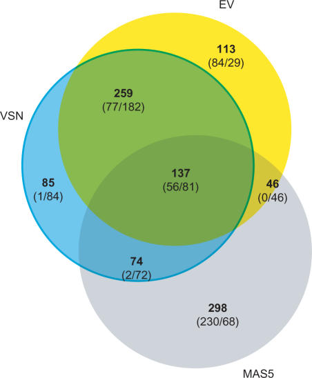
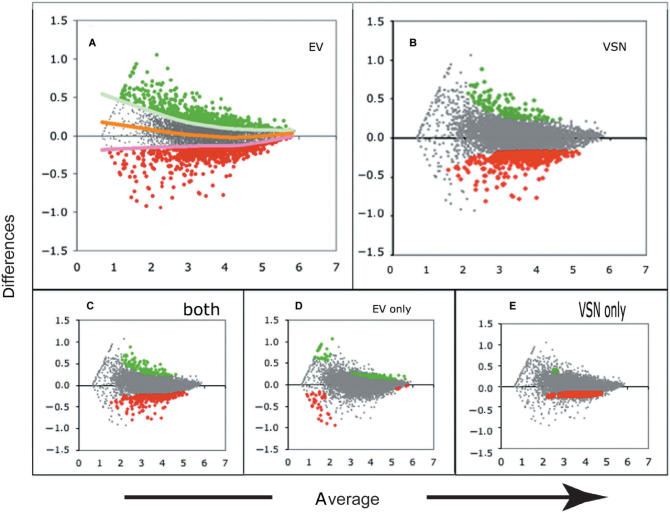
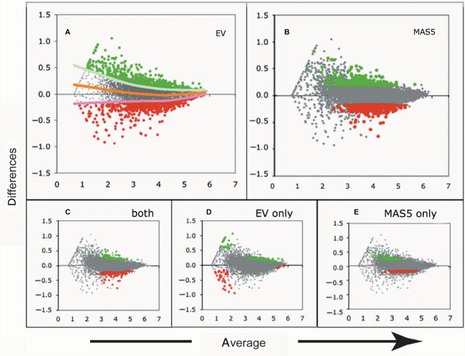
When 555 genes selected with each of the methods, comparison between the selected sets with VSN and EV shows that 396/555 genes were common to both methods (Figure 3). Furthermore, comparison of the gene sets selected by MAS5 and EV indicated that 183/555 genes were common to MAS5 and EV (Figure 3). Interestingly, these comparisons also show that whereas VSN selects a higher fraction of down-regulated genes as compared to MAS5 and EV (Figure 4B), whereas MAS5 selects a higher fraction of up-regulated genes from the same dataset (Figure 5B). EV, however, is able to select a similar number of over- and down-regulated genes (Figures 4A and 5A). It is conceivable that the differences between EV and VSN could be related to the fit to the actual distribution of the data adopted by either method. Indeed, the distribution of the analyzed dataset was ‘banana shaped’ and whereas EV is fitted to the median, the selection on VSN-transformed data was centered around 0, resulting in selection differences in the median range of expression (Figure 4). A difference was also noted in the selection efficiency at low- and high-expression ranges (Figure 4D and E), where EV identifies as regulated, genes not identified by VSN. These differences can be related to differences in variance stabilization. The differences between EV and MAS5 could be related to normalization on the variance distribution of the data adopted by either method. MAS5 did not select the lowest or highest expressed genes. It only selected genes expressed at intermediate levels (Figure 5E), as previously reported by others (22).

Figure 3.

Comparison of differentially expressed genes selected with EV, VSN and MAS5. A set of 555 differentially expressed genes was selected from an Affymetrix-generated dataset either with EV, VSN-transformed data, and MAS5. Each analysis is represented by a colored circle. The intersections represent the overlaps between the different analysis methods. Numbers in bold correspond to the total number of genes detected on each compartment, whereas values between brackets indicate the up- and down-regulated genes respectively.

Figure 4.

Differentially expressed genes selected on spline (EV) or VSN transformed data. The same dataset represented in Figure 2 was used to select differentially expressed genes on spline (EV) or VSN-transformed data. MA plots of scaled log-transformed signals for probe sets from two experimental conditions of the B6.1 cells. Color codes are as in Figure 1. Up-regulated genes are shown as green bold dots, down-regulated as red bold dots. (A) Distribution of 555 genes (P-value = 0.05) selected upon a spline fit. (B) Distribution of 555 genes (FC = 1.63) on VSN-transformed data. (C) Distribution of genes selected by both approaches. (D) Distribution of genes selected by EV (spline fit) alone. (E) genes selected by VSN (arcsinh transformation) alone.

Figure 5.

Differentially expressed genes selected using spline or MAS5 Affymetrix selection. MA plots of scaled log-transformed signals for probe sets from two experimental conditions of the B6.1 cells, using the same dataset and color codes as in Figure 4. (A) Distribution of 555 genes (P-value = 0.05) selected upon a spline fit. (B) Distribution of 555 genes selected by MAS5 (FC = 1.8). (C) Distribution of genes selected by both approaches. (D) Distribution of genes selected by EV (spline fit) alone. (E) Genes selected by FC on MAS5 alone.

Specificity and sensitivity of EV as compared to MAS5 and VSN

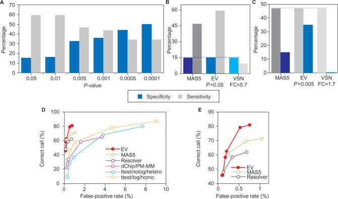
The U133 Latin square dataset from Affymetrix (see Materials and Methods section) was used to demonstrate the specificity and sensitivity of EV. Indeed, analysis of experiments with the lowest changes in the concentration of the spikes (2-fold, i.e. comparison of experiments 1 and 2), showed a large increase in specificity, concomitant with a moderate sensitivity decrease with decreasing P-values ranging from 0.05 to 0.0001 (see Figure 6A). Furthermore, with increasing FC of the spikes (2-fold: experiments 1 and 2; 4-fold: experiments 1 and 3; 8-fold: experiments 1 and 3), there is a large increase in specificity, concomitant with a more moderate increase in specificity (not shown). In addition, to directly assess EV performance, it was decided to compare in one hand the sensitivity of the different methods for a given specificity (Figure 6B), and on the other hand, the specificity for a given sensitivity (Figure 6C). Indeed, when the specificity was fixed for all the methods at 15% (value obtained with MAS5), EV (P = 0.05) showed a 1.27-fold higher sensitivity than MAS5 and 6.32-fold higher than VSN (Figure 6C). Furthermore, when the sensitivity was fixed for all the methods at 47% (value obtained with MAS5), EV (P = 0.005) showed a higher specificity than MAS5 (2.3-fold) and VSN (58-fold) (Figure 6D). EV performance, in terms of sensitivity and specificity, was systematically compared with other methods in addition to VSN and MAS5. These comparisons were made constructing receiver operatic characteristics (ROC) curves, where the overall accuracy or sensitivity across a range of P-value cutoffs is plotted on the y-axis, whereas the false-positive rate (FPR), assessed from the number of transcripts not included in the Latin square set that are determined to have changed significantly, is shown on the x-axis. EV performance was compared with MAS5 (21,23), Rosetta Resolver (24,25), dChip/PM-MM (26), and two versions of the two-tailed t-test: the heteroscedastic version without log transformation of the intensities (ttest/nolog/hetero) and the homoscedastic version after log transformation (ttest/log/homo). Rajagopalan (27) has already shown that in this type of analyses, MAS5 and Resolver have a superior performance than dChip or t-tests. Our data shows that this is also true for EV (Figure 6D). Indeed, at a fixed FPR, chosen for comparison purposes, within the same range as obtained with other methods, EV detects many more true changes, not only than dChip and t-tests, but also than MAS5 and Resolver (Figure 6D and E), in particular for FPR rates higher than 0.12 for Resolver or FPR higher than 0.25 for MAS5. Conversely, to obtain a comparable level of accuracy, MAS5, Resolver, dChip and t-tests would generate many more false-positive calls (Figure 6D and E). Furthermore, EV was not outperformed by other methods on any of the analyses we have carried out so far.

Figure 6.

Sensitivity and specificity of EV determined on the Affymetrix Latin square dataset. Data from a Latin square experiment available from Affymetrix (see Materials and Methods section), where 42 human genome U133 chips were hybridized with three technical replicates of 14 separate hybridizations of 42 spiked transcripts in a complex human background at concentrations ranging from 0.125 to 512 pM was used to determine the sensitivity and specificity of EV, as compared to MAS5 and VSN. (A) Changes of specificity (blue) and sensitivity (gray) in EV analyses with a 2-fold change in the concentration of spikes. The data presented corresponds to the comparison of experiments 1 and 2, but is representative of comparison between experiments n and n + 1 (corresponding to spikes with 2-fold change). (B) Direct comparison of sensitivity changes (gray) at a fixed specificity (blue) for the dataset analyzed with MAS5, EV and VSN. (C) Direct comparison of specificity changes (blue) for a fixed sensitivity (gray) for the dataset analyzed with MAS5, EV and VSN. (D) Comparison of EV performance with MAS5, Resolver, dChip/PM-MM, t-test/nolog/hetero and t-test/log/homo in terms of sensitivity and specificity, using P-value cutoffs for each (0.0025, 0.005, 0.01, 0.05, 0.1) and represented as receiver operatic characteristics (ROC) curves. The overall accuracy or sensitivity across all concentrations is plotted on the y-axis versus the false-positive rate (x-axis), determined from the number of transcripts not included in the Latin square set that are determined to have changed significantly. (E) Detail from the graph depicted in (D).

DISCUSSION

In expression profiling analyses, outlining proper thresholds to determine differential expression, avoiding false positives, still remains one of the major issues to be solved. One of the problems encountered with DNA array datasets is the unequal distribution of the variance, which is inversely proportional to the log of intensities, consequently affecting threshold settings for differential expression. In the analysis of expression profiling datasets, the central issue comes down to building confidence intervals that successfully fit the variability due to noise (experimental or technological). One way to solve the problem is to mathematically transform the data in order to normalize the variance.

Here, we propose the use of the normalized value of the expression level (EV), a model for micro-array data processing based on spline functions, which has proved its ability to provide models for complex phenomena (28) and curve fitting in data analysis of observations with random components. The examples analyzed with EV show that, due to the Box–Cox spline transformation, the transformed data shows a normal distribution, and allows the definition of a continuous confidence band delineating the DS, the interval including all genes devoid of significant expression changes, which can be adjusted to a standard deviation. The values (x_i, y_i) for each gene in the dataset not included in DS (located outside the upper or lower spline curves) is then associated with a P-value, which provides statistical support for the selection of outliers.

The specificity and sensitivity of EV were determined analyzing the U133 Latin square dataset from Affymetrix. The dataset was generated from the hybridization of 42 human genome chips with 3 technical replicates of 14 separate hybridizations, obtained from a human RNA containing 42 spiked transcripts at concentrations ranging from 0.125 to 512 pM. These comparisons demonstrate that EV was more robust than MAS5 and VSN in this type of analysis. Indeed, when analyzing experiments in which the spikes had a 2-fold change, for a fixed specificity EV showed a 1.27-fold and 6.32-fold higher sensitivity than MAS5 and VSN, respectively (see Figure 6B); and for a fixed sensitivity, EV was 2.3-fold and 58-fold higher specificity than MAS5 and VSN, respectively (see Figure 6C). Performance of EV was also directly compared to MAS5, Resolver, dChip and two types of t-test analyses, showing also a better performance than these tests (Figure 6D and E). The specificity of EV showed a large increase with the increase of FC in the spikes, concomitant with a moderate increase in specificity (not shown).

The comparison of EV, VSN and MAS5 data analysis from a real expression profiling experiment (B6.1-arrays), comparing the profiles of exponentially growing and G1-arrested cells (Figures 3–5) gave a slightly different picture. In this experiment, EV leads to a more robust variance stabilization than VSN; in addition, EV leads to an increase in the homogeneity of the selected sets, and thus to an increased reproducibility on the selection of outliers. In this experiment, however, the direct comparison of the three methods, clearly shows that EV and VSN are closer (71%) than MAS5, whereas the coincidences between EV and MAS5, or VSN and MAS5 are 33 and 38% respectively. The differences between EV and VSN are mainly due to the fact that EV takes into account the shape of the diagonal in the form of concave or convex distortions. In the small fraction of datasets devoid of such distortions, there are virtually no differences in the set of selected genes (not shown), and VSN performs definitively better in this experiment than in the Latin square data analysis. The data reported here also demonstrate that, unlike classical approaches such as MAS5, EV does not encounter any difficulty on selecting regulated genes with either high- or low-expression levels.

Furthermore, in two analyses in which chips hybridized with RNAs obtained from cells grown in two different conditions (A and B), and the set of selected genes was compared with another dataset in which the datasets compared were 10xA and B. It is relevant that in both comparisons, the set of identified genes was rigorously the same (>98% identities) (not shown). This demonstrates, not only the strength and robustness of EV on variance stabilization, and might allow to compare data obtained under different conditions, and even datasets generated with chips from different origins.

For physiological and pathological processes, in general there is no a priori evidence for a higher number of up-regulated or down-regulated genes. Normalization of the distribution by the Box–Cox transformation makes globally a symmetric distribution of expression datasets, although at the extremes of this distribution, asymmetries are often detected. Moreover, it is possible to force an asymmetric selection, by using different sets of tuning parameters (EV thresholds), when there is information suggesting that the ‘treatment’ will lead to a larger number of either up-regulated or down-regulated genes. It should also be noted that the selection of genes is only one of the steps in the process of data analysis, the data should be strengthened by replicated analysis with other biological samples, and subsequently validated by northern, western, Q-PCR, etc.

In conclusion, splines seem to be well adapted for micro-array analyses since, (i) the transformed data shows a normal distribution and the median axis overlaps the first diagonal; (ii) it results in a robust variance stabilization; (iii) its usage is independent of the number of genes present on each dataset and the technological origin of the arrays; (iv) they are defined piecewise and are more adjusted to local distortions of the data, thus improving the fit; (v) the width of DS can be adjusted by changing the values of the parameter α; and (vi) asymmetric selection of up-regulated or down-regulated genes can be forced by changing the tuning parameters. We, thus, propose that EV could play a pivotal role in expression profiling data analysis, since it overcomes many of the difficulties shown by other methods on selecting differentially expressed genes.

REFERENCES

- 1.Balding DJ, Bishop M, Cannings C. Handbook of Statistical Genetics. 2nd edn. vol 1. John Wiley & Sons, West Sussex; 2003. [Google Scholar]
- 2.Munson P. A consistency test for determining the significance of gene expression changes on replicate samples and two convenient variance-stabilizing transformation.. Conference Proceedings: GeneLogic Workshop on Low Level Analysis of Affymetrix GeneChip Data; Bethesda, Maryland. 2001. [Google Scholar]
- 3.Durbin BP, Hardin JS, Hawkins DM, Rocke DM. A variance-stabilizing transformation for gene-expression microarray data. Bioinformatics. 2002;18(Suppl. 1):S105–S110. doi: 10.1093/bioinformatics/18.suppl_1.s105. [DOI] [PubMed] [Google Scholar]
- 4.Hawkins DM. Diagnostics for conformity of paired quantitative measurements. Stat. Med. 2002;21:1913–1935. doi: 10.1002/sim.1013. [DOI] [PubMed] [Google Scholar]
- 5.Huber W, Von Heydebreck A, Sultmann H, Poustka A, Vingron M. Variance stabilization applied to microarray data calibration and to the quantification of differential expression. Bioinformatics. 2002;18(Suppl. 1):S96–S104. doi: 10.1093/bioinformatics/18.suppl_1.s96. [DOI] [PubMed] [Google Scholar]
- 6.Mills JC, Gordon JI. A new approach for filtering noise from high-density oligonucleotide microarray datasets. Nucleic Acids Res. 2001;29:E72–72. doi: 10.1093/nar/29.15.e72. [DOI] [PMC free article] [PubMed] [Google Scholar]
- 7.Bertucci F, Van Hulst S, Bernard K, Loriod B, Granjeaud S, Tagett R, Starkey M, Nguyen C, Jordan B, et al. Expression scanning of an array of growth control genes in human tumor cell lines. Oncogene. 1999;18:3905–3912. doi: 10.1038/sj.onc.1202731. [DOI] [PubMed] [Google Scholar]
- 8.Cole TJ, Green PJ. Smoothing reference centile curves: the LMS method and penalized likelihood. Stat. Med. 1992;11:1305–1319. doi: 10.1002/sim.4780111005. [DOI] [PubMed] [Google Scholar]
- 9.Tukey JW. Anatomy of transformations. Ann. Math. Statist. 1957:602–632. [Google Scholar]
- 10.Box GEP, Cox DR. An Analysis of transformations. J. Roy. Stati. Soc. B. 1964;78:211–243. [Google Scholar]
- 11.Cole TJ. The LMS method for constructing normalized growth standards. Eur. J. Clin. Nutr. 1990;44:45–60. [PubMed] [Google Scholar]
- 12.Wegman EJ, Wright IW. Splines in statistics. J. Am. Stati. Assoc. 1983;78:351–365. [Google Scholar]
- 13.Nürnberger G. Approximation by spline functions.. Conference Proceedings; Springer, Berlin. 1989. [Google Scholar]
- 14.Zhang L, Zhou W, Velculescu VE, Kern SE, Hruban RH, Hamilton SR, Vogelstein B, Kinzler KW. Gene expression profiles in normal and cancer cells. Science. 1997;276:1268–1272. doi: 10.1126/science.276.5316.1268. [DOI] [PubMed] [Google Scholar]
- 15.Stremmel C, Wein A, Hohenberger W, Reingruber B. DNA microarrays: a new diagnostic tool and its implications in colorectal cancer. Int. J. Colorectal Dis. 2002;17:131–136. doi: 10.1007/s00384-001-0370-7. [DOI] [PubMed] [Google Scholar]
- 16.von Boehmer H, Hengartner H, Nabholz M, Lernhardt W, Schreier MH, Haas W. Fine specificity of a continuously growing killer cell clone specific for H-Y antigen. Eur. J. Immunol. 1979;9:592–597. doi: 10.1002/eji.1830090804. [DOI] [PubMed] [Google Scholar]
- 17.Karasuyama H, Melchers F. Establishment of mouse cell lines which constitutively secrete large quantities of interleukin 2, 3, 4 or 5, using modified cDNA expression vectors. Eur. J. Immunol. 1988;18:97–104. doi: 10.1002/eji.1830180115. [DOI] [PubMed] [Google Scholar]
- 18.Müllner EW, Garcia-Sanz JA. In: Manual of Immunological Methods. Lefkovits I, editor. Vol. 1. London: Academic Press; 1997. pp. 389–406. [Google Scholar]
- 19.Müllner EW, Garcia-Sanz JA. In: Immunology Methods Manual. Lefkovits I, editor. Vol. 1. London: Academic Press; 1997. pp. 407–424. [Google Scholar]
- 20.Sauvonnet N, Pradet-Balade B, Garcia-Sanz JA, Cornelis GR. Regulation of mRNA expression in macrophages after Yersinia enterocolitica infection. Role of different Yop effectors. J. Biol. Chem. 2002;277:25133–25142. doi: 10.1074/jbc.M203239200. [DOI] [PubMed] [Google Scholar]
- 21.Hubbell E, Liu WM, Mei R. Robust estimators for expression analysis. Bioinformatics. 2002;18:1585–1592. doi: 10.1093/bioinformatics/18.12.1585. [DOI] [PubMed] [Google Scholar]
- 22.Shedden K, Chen W, Kuick R, Ghosh D, Macdonald J, Cho KR, Giordano TJ, Gruber SB, Fearon ER, et al. Comparison of seven methods for producing Affymetrix expression scores based on false discovery rates in disease profiling data. BMC Bioinformatics. 2005;6:26. doi: 10.1186/1471-2105-6-26. [DOI] [PMC free article] [PubMed] [Google Scholar]
- 23.Liu WM, Mei R, Di X, Ryder TB, Hubbell E, Dee S, Webster TA, Harrington CA, Ho MH, et al. Analysis of high density expression microarrays with signed-rank call algorithms. Bioinformatics. 2002;18:1593–1599. doi: 10.1093/bioinformatics/18.12.1593. [DOI] [PubMed] [Google Scholar]
- 24.Stoughton R, Dai H. Statistical combining of cell expression profiles. US Patent. 2002;6:351–712. [Google Scholar]
- 25.Roberts CJ, Nelson B, Marton MJ, Stoughton R, Meyer MR, Bennett HA, He YD, Dai H, Walker WL, et al. Signaling and circuitry of multiple MAPK pathways revealed by a matrix of global gene expression profiles. Science. 2000;287:873–880. doi: 10.1126/science.287.5454.873. [DOI] [PubMed] [Google Scholar]
- 26.Li C, Wong WH. Model-based analysis of oligonucleotide arrays: expression index computation and outlier detection. Proc. Natl. Acad. Sci. USA. 2001;98:31–36. doi: 10.1073/pnas.011404098. [DOI] [PMC free article] [PubMed] [Google Scholar]
- 27.Rajagopalan D. A comparison of statistical methods for analysis of high density oligonucleotide array data. Bioinformatics. 2003;19:1469–1476. doi: 10.1093/bioinformatics/btg202. [DOI] [PubMed] [Google Scholar]
- 28.Eubank RL. Approximate regression models and splines. Comm. Statist. Theor. Methods. 1984;13:433–484. [Google Scholar]