A new approach for filtering noise from high-density oligonucleotide microarray datasets

Abstract

Although DNA microarrays are powerful tools for profiling gene expression, the dynamic range and the sheer number of signals produced require efficient procedures for distinguishing false positive results (noise) from changes in expression that are ‘real’ (independently reproducible). We have developed an approach to filter noise from datasets generated when high density oligonucleotide-based microarrays are used to compare two distinct RNA populations. First, we performed comparisons between chips hybridized with cRNAs prepared from an identical starting RNA population; an ‘Increase’ or ‘Decrease’ call in such a comparison was defined as a false positive. Plotting the average distribution of these false positive signal intensities across 18 such comparisons of nine independent RNA preparations allowed us to develop a series of noise-filtering look-up tables (LUTs). Using a database of 70 separate chip-to-chip comparisons between distinct RNA preparations prepared by different workers at different sites and at different times, we show that the LUTs can be used to predict the likelihood that a given transcript called Increased or Decreased in one comparison will again be called Increased or Decreased in a replicate comparison. Evidence is presented that this LUT-based scoring system provides greater predictive value for reproducible microarray results than imposition of arbitrary fold-change thresholds and accurately predicts which microarray-identified changes will be validated by independent assays such as quantitative real-time PCR.

INTRODUCTION

The use of high-density DNA microarrays for profiling expression of thousands of genes in tissues and cells has increased dramatically in the few years since their introduction. The broad-based, comprehensive profiling of cellular mRNA transcripts made possible by microarrays can provide unanticipated insights about the molecular mechanisms that regulate cellular function. However, the impressive quantity of data microarrays provide is associated with a substantial amount of noise (1). To illustrate, a microarray-based comparison of two RNA samples prepared prior to and after an experimental manipulation often yields a list of a few hundred mRNAs whose levels appear to be changed. Given that microarrays often monitor up to 10 000 genes at a time, a false positive rate as low as 1% will result in 100 false difference calls (2). Thus, noise can often rival signal in large-scale gene expression profiling. It is clearly not practical to confirm every change identified in a microarray-based comparison with independent and time-consuming assays. Systematic approaches to distinguish false positives (noise) from changes that are real (independently reproducible) are needed (3–5).

The most common strategy for decreasing noise in microarray-based comparisons is to establish an arbitrary global threshold for fold-change (typically 2–3-fold). An individual mRNA species has to equal or exceed this mandated level of difference between control and experimental RNA preparations before it is considered to have undergone a change that is likely to be true (6,7). There are several limitations to this approach, not least of which is that applying an arbitrary cut-off may mask biologically significant changes (see Discussion for more details) (3,4).

In this report, we have used datasets generated with commercially available high-density oligonucleotide-based microarrays as an experimental model to develop a new systematic, empirically-based approach for identifying noise. There were several reasons why a commercial, oligonucleotide-based microarray was selected. First, these GeneChip microarrays (www.affymetrix.com) are used widely for a variety of experimental applications (8). Secondly, they are mass-produced and contain a robust series of controls designed to minimize chip-to-chip variation. Briefly, each gene is represented by at least one probe set that is composed of multiple (∼20) oligo probe pairs. Each probe pair consists of two 25 base sequences, one perfectly complementary to a portion of a given transcript, the other with all but the 13th base matching the transcript. Signal produced by hybridization to a mismatch probe is considered noise, and serves as an internal control for the signal produced by the corresponding perfect match probe. Finally, GeneChips are supported by a proprietary software package that provides extensive information about each probe set.

We have analyzed this probe-set specific information, which comes in the form of several parameters, to devise a method for algorithmically defining noise in any given single GeneChip array. We show that our approach to noise filtration not only permits an experiment-wide assessment of overall data quality, but also allows the user to score and rank individual genes according to their likelihood of manifesting changes that are reproducible.

MATERIALS AND METHODS

Preparation of cRNA targets and hybridization

Total cellular RNA was isolated (RNeasy kit, Qiagen) from five different mouse tissues under several different conditions: (i) distal small intestine of germ-free adult NMRI mice prior to, or 10 days after, colonization with Bacteroides thetaiotaomicron, Escherichia coli or a complete intestinal microflora (9); (ii) liver from germ-free mice prior to and 10 days after intestinal colonization with a conventional gut microflora; (iii) age-matched stomachs from (a) adult germ-free FVB/N mice, (b) germ-free FVB/N transgenic mice that express the human histoblood group antigen, Lewis^b, in gastric pit cells (10) and (c) germ-free transgenic mice that have an engineered ablation of their acid-producing gastric parietal cells (11); (iv) stomachs of age-matched mice belonging to groups (a)–(c) but 8 weeks after colonization with a clinical isolate of the human gastric pathogen Helicobacter pylori; (v) gastric parietal cell-enriched and -depleted fractions generated by lectin panning of stomach mucosa harvested from: conventionally-raised normal FVB/N mice, ex-germ-free normal FVB/N mice 2 and 8 weeks after H.pylori infection, and age-matched germ-free controls (J.Mills, A.J.Syder, C.V.Hong, F.Raaii, and J.I.Gordon, manuscript in preparation); and (vi) the bladders of adult female C57Bl6 mice before and 1.5 or 3.5 h after infection with either a clinical isolate of uropathogenic E.coli that expresses the FimH adhesin (NU14) or a FimH-negative isogenic strain (NU14-1) (12).

‘Analytic duplicates’ were prepared as follows. Equal amounts of RNA, prepared from each mouse in a given control or treatment group were pooled. Each single RNA pool was then divided into two equal portions (30 µg/portion). Biotinylated cRNA targets were prepared independently from each 30 µg sample, using the protocol outlined previously (13). ‘Biological duplicates’ represented two independently isolated pools of RNA from two different groups of animals. Each of the two groups had been subjected to the same control or experimental conditions.

All cRNAs were hybridized to Affymetrix Mu11KsubA and Mu11KsubB chip sets according to protocols recommended by Affymetrix. Data from each chip were scaled so that the overall fluorescence intensity across each chip was equivalent (average target intensity set at 150).

RESULTS

Initial definition of noise: comparing microarrays probed with duplicate cRNA targets

During the analytic phase of a microarray comparison (i.e. after a biological sample has been collected), noise can be generated at multiple steps including chip manufacture, preparation of cRNAs for microarray interrogation, hybridization or washing steps, and global normalization of overall signal intensities between chips. In this report, we have taken an empirical approach to defining noise to ensure that each of the potential analytic noise-generating steps would be considered.

Numerous GeneChip datasets were generated, using the scheme in Figure 1. The datasets comprise the work of two different investigators, with RNA processing and chip hybridization occurring at two independent laboratories at different times. The tissue source was the gastrointestinal tracts of inbred strains of mice having four distinct genetic backgrounds. For each genetic background, ‘treated’ RNA was prepared from groups of mice (n = 5/group) that had been subjected to a physiological or pathophysiological manipulation. RNA was also isolated from a group of unmanipulated control animals.

Figure 1.

Summary of scheme used to generate duplicate Same–Same comparisons. (A) outline of origins of RNA preparations used for Same–Same comparisons. (B) Flow chart of how RNAs, generated from mice of given genetic background were processed to produce duplicate GeneChip hybridizations. (C) Schemes used to generate Same–Same comparisons for A chips. One of the approaches employed to compare biologically distinct RNAs is also illustrated (labeled ‘true different’). Identical approaches were used for B chip comparisons.

Figure 1A lists the nine treated and untreated RNAs from the four different inbred strains. Equal-size aliquots from each RNA were used as templates to independently prepare two ‘target’ cRNAs (target refers to the cRNA produced from an RNA sample; ‘probe’ refers to the oligonucleotides represented in the microarray). Each of the duplicate cRNA targets was then hybridized to the two chips (A and B) that together comprise the Affymetrix Mu11K GeneChip set (Fig. 1B). The combined A and B chips represent ∼11 000 mouse genes from Unigene Build 4.

After hybridizing the two cRNAs generated from the same RNA sample to two separate A chips, the expression profiles generated from the two A chips were compared to one another. These comparisons were termed ‘Same–Same’ (Fig. 1C). A similar approach was used for the B chips. Differences in gene expression identified from such Same–Same comparisons were defined as noise (see below). Thus, the nine RNAs yielded a bank of 18 interrogated A chips and nine A chip Same–Same comparisons, plus a similar number of interrogated B chips and B chip Same–Same comparisons.

Same–Same comparisons among the 36 chips were performed using standard protocols for GeneChips. Briefly, GeneChip software was used to perform a scaling operation that (i) measured the intensity of each signal generated by each probe set on the chip and (ii) defined an average value across the entire array. A global scaling was then performed by the software so that all probe set signal intensities, across the chip, were adjusted to produce a new (scaled) average intensity for the chip that was shared by all other scaled chips. In theory, once chips in a Same–Same comparison are scaled to a common average intensity, the signal produced by any individual gene transcript on one chip can be directly compared to the intensity of that transcript on a ‘Partner’ chip. Because the scaling procedure itself could be an important generator of noise (see below), we standardized the nomenclature and procedure for all Same–Same comparisons. The chip with the higher scaling factor was always designated as the ‘Baseline’ chip. The higher scaling means that the Baseline chip had a lower intensity on average than its Partner chip and, therefore, was multiplied by a higher scaling factor to reach the arbitrarily selected, chip-wide average intensity value.

As noted in the Introduction, GeneChips contain multiple internally controlled probes for each gene [the typical probe set for a gene consists of 20 perfect match (PM) oligos and 20 corresponding single base mismatch (MM) oligos]. For a given transcript in any given chip-to-chip comparison, GeneChip software generates a ‘Difference call’ parameter (Increase or Decrease) based on a consideration of signal specificity as well as intensity. In other words, the call is based on an evaluation of the intensities of the signals generated from each PM oligo versus each MM oligo on one chip relative to the corresponding PM versus MM signal intensities on the other chip. If cRNA target generation and hybridization/washing steps were reproducible, and if the scaling procedure did not introduce any artifacts, then there should be no differences in expression levels detected by any of the probe sets represented on the two chips in a Same–Same comparison. Accordingly, transcripts called Increased in a Same–Same comparison represent instances where the signal on the higher intensity (Partner) chip is falsely elevated. Decrease calls represent instances where the signal on the lower intensity (Baseline) chip has been falsely elevated. We defined all Increase or Decrease calls in a Same–Same comparison as false positives.

Table 1 presents results obtained from the nine Same–Same comparisons involving 18 chip pairs. For example, when the duplicate cRNAs generated from RNA preparation 1 (Fig. 1A and B, Genetic Background #1, untreated RNA), were compared using two A chips, 870 of the 6508 probe sets yielded Difference calls (overall false positive rate = 13%). Of these, 799 were called Increased when the Partner chip with overall higher intensity signals from its probe sets was compared to the Baseline chip with overall lower intensity signals. [The scaling factor ratio (SFR) shown in Table 1 refers to the ratio of the Baseline chip’s scaling factor to its Partner’s scaling factor.] Decrease calls in the Same–Same comparison involving RNA preparation 1 were produced by 71 probe sets.

Table 1. Summary of Difference calls in all nine Same–Same comparisons.

RNA prep #	Total	Increased	Decreased	% False positive	SFR	≥2-fold difference
						Total	% False positive
A chip
1	870	799	71	13	10.12	447	7
2	787	717	70	12	5.21	322	5
3	1028	955	73	16	6.04	477	7
4	853	779	74	13	4.81	382	6
5	359	291	68	6	1.86	158	2
6	159	16	143	2	1.04	86	1
7	87	41	46	1	1.2	33	1
8	1282	1206	76	20	3.01	636	10
9	1437	1308	129	22	2.34	832	13
B chip
1	293	182	111	4	1.47	167	3
2	323	166	157	5	1.7	182	3
3	247	153	94	4	1.6	120	2
4	97	71	26	1	12.7	44	1
5	141	104	37	2	2.32	61	1
6	209	175	34	3	4.71	115	2
7	71	41	30	1	1.15	41	1
8	204	117	87	3	2.27	107	2
9	713	431	282	11	1.39	485	7

Each starting RNA was split in two and applied to two separate A chips and two separate B chips (see Fig. 1). The two A chips were compared to each other, and the total number of Difference calls determined. The same was done for the B chips. ‘Total’, total Difference calls, irrespective of fold-change; ‘% False positive’, total Same–Same Difference calls expressed as a percentage of total probe sets on chip; ‘SFR’, the ratio of the Baseline chip scaling factor divided by that of its Partner (a measure of the relative difference in overall intensity between the two Same–Same chips).

Same–Same comparisons involving the nine RNAs and the A and B chips resulted in a mean false positive percentage of 8 ± 7% (range = <1–22%; see Table 1). The mean false positive percentage was reduced to 4 ± 3% when the criterion of ≥2-fold change was imposed on transcripts called Increased or Decreased. Even with this added stringency, 7/9 Same–Same comparisons involving the A chips, and 6/9 of Same–Same comparisons involving the B chips produced >100 false positive changes (Table 1).

Identifying the source of false positives

In 16/18 of the Same–Same comparisons, the vast majority of the difference calls were Increases. Because the lower intensity chip was designated as the Baseline, this finding suggested that scaling may have introduced artifacts that contributed to noise in a non-random way.

For transcripts whose intensities are within the range of detection on both chips, scaling should work well to standardize chip-to-chip variation, and such transcripts should be read as ‘No Change’ in Same–Same comparisons (e.g. Fig. 2 lines colored teal). However, we reasoned that with chip-wide scaling, two types of errors are bound to affect probe sets (transcripts) at the extremes of intensities. First, without scaling, many transcripts that are just over the threshold of detection on the higher intensity Partner chip will be below the level of detection on the low intensity Baseline chip. No amount of scaling can reliably increase transcript intensities that are below detection (multiplying zero by any number still gives zero; e.g. Fig. 2, red lines). Thus, in a Same–Same comparison, these pairs of near-threshold transcripts will be falsely called Increased over Baseline after scaling (designated low signal intensity scaling factor errors). Secondly, genes that are above the linear range of signal intensity on the higher intensity chip may still be near this threshold on the lower intensity chip. Multiplying such transcripts by a scaling factor will result in falsely elevated Baseline intensities and, thus, false Decrease calls (designated high signal intensity scaling factor errors; Fig. 2, dark blue line). Note that array-wide scaling is not specific to Affymetrix GeneChips. Any scaled comparison of microarrays with genes at or outside the linear range of detection will be prone to these two types of error (i.e. as SFRs increase, the number of false positives should also rise).

Figure 2.

Predicted effects of global scaling on Difference calls. Each line connects signal intensities of corresponding probe sets in a pair of chips used for a Same–Same comparison. Different colors represent different consequences of global scaling. Signal intensity is expressed in arbitrary units to allow comparison of the left and right panels. For the purposes of illustration, prior to scaling, the average signal intensity of the Baseline chip was set at 2-fold lower than its Partner chip. The average intensity of the Partner chip was set at the designated scaling target intensity. Thus, after scaling, the intensity values of all of the probe sets on the Baseline chip rise 2-fold, while the values on the Partner chip do not change.

An initial approach for distinguishing true positives from noise

To develop strategies for minimizing false positive calls, we first characterized (i) a dataset of all transcripts called Increased in a Same–Same comparison and (ii) a dataset of all Increased calls produced from comparison of two biologically distinct RNAs. The characterization involved plotting a transcript’s intensity on the scaled Baseline chip as a function of its intensity on the scaled Partner chip (intensity is defined by GeneChip software as the ‘Average Difference’ for all PM versus MM oligos across the probe set recognizing a given transcript).

Figure 3 presents an example of such a scatter plot comparing two datasets: one representing Increased calls from a Same–Same A chip comparison obtained from RNA preparation 1; the other representing Increased calls from a comparison of biologically distinct RNAs (Fig. 1C, a ‘true different’ comparison). Figure 3 shows that the transcripts called Increased in the Same–Same comparison generally have lower intensities on the Partner chip than do the transcripts called Increased in the comparison of the biologically distinct RNA preparations. Moreover, the Same–Same transcripts called Increased cluster near relatively low Baseline chip intensity values (<250; low signal intensity scaling factor errors would be predicted to contribute to this clustering at low Baseline chip intensity values). These findings were not unique to the Same–Same dataset shown in Figure 3: similar results were obtained with all the other Same–Same datasets (i.e. from RNA preparations 2–9; data not shown).

Figure 3.

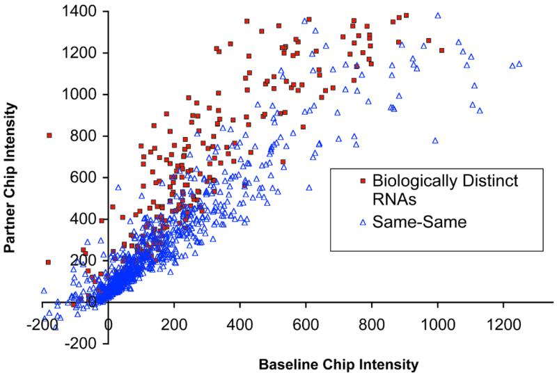
Distribution of signals produced from a single Same–Same comparison compared to signals produced from a comparison of two biologically distinct RNAs. Data represent probe sets that gave an Increase call on A chips. Signal intensity for a probe set represented on the scaled Baseline chip is plotted as a function of the corresponding intensity of the probe set represented on the scaled Partner chip.

Given the apparent non-random distribution of noise in these plots, we proceeded to standardize the process of differentiating Same–Same comparisons from comparisons of two biologically distinct RNAs. To do so, a grid was generated that subdivided the entire range of Baseline chip and Partner chip intensities. We first considered the cohort of all Increased calls in a given Same–Same comparison. Baseline chip transcript intensity was plotted on the x-axis of the grid: intensities were divided into 22 arbitrarily defined groupings that together encompassed the full range of possible Baseline intensity values. Partner chip intensities were plotted on the z-axis of the grid, with values collated into ≤8 arbitrarily defined groupings. [To systematize division of Partner chip intensities into these groups, the entire range of these intensities was first assigned values of 0–53 based on the following scheme. After Partner chips were subjected to global scaling, Partner chip intensity values ≤0 were redefined as having a value of 0 (Affymetrix software uses the Average Difference between all perfect match and mismatch probe pairs across a probe set to determine probe set/transcript intensity; thus, negative intensities are possible). For Partner chip probe set intensities ≥0, values were redefined in increments of 50 (i.e. 1–50 = 1, 51–100 = 2) up to values of 1000 (951–1000 = 20). The same approach was used for values of 1001–2000, but the increment was 100 (e.g. a Partner chip intensity of 1950 was re-assigned 30). From 2001–4000, the increment for grouping was 200 (intensity of 3650 = 39). From 4001–8800, the increment was 400 (e.g. 5301 = 44). All Partner intensities >8800 were redefined as 53. The iterative nature of this scheme permitted rapid conversion of each Partner chip probe set intensity value (from the GeneChip software Average Difference parameter) to the redefined value with a short series of simple ‘For...Next’ loops in the Excel macro language, Visual Basic for Applications (VBA). Bins were created using Baseline chip intensity groupings and combinations of the redefined Partner chip values. For example, for the 0–50 Baseline chip intensity grouping (one of the most common), eight Partner chip groupings were used. Partner chip group 1 (representing the lowest possible Partner chip intensities in that Baseline grouping) included all Partner chip intensities with redefined values of ≤1. Partner chip group 2 contained redefined Partner chip intensities of 2. Groups 3, 4 and 5 contained redefined intensities of 3, 4 and 5, respectively. Group 6 included redefined Partner chip intensities values of 6 and 7, group 7 contained redefined values of 8 and 9, while group 8 included all redefined values ≥10.] The y-axis of the grid was used to plot Increase calls at each x–z coordinate as a fraction of the total Increase calls represented on the whole grid. The histogram in Figure 4A represents the mean distribution of all Increase calls obtained for each of the nine A chip Same–Same comparisons. Figure 4C shows the corresponding plot for the B chip Same–Same comparisons. Figure 4B and D provide analogous compiled data for comparisons of several sets of biologically distinct RNAs.

Figure 4.

Three-dimensional plots of Baseline chip and Partner chip intensities for a Same–Same comparison and for a comparison of biologically distinct RNAs. Probe sets producing Increase or Decrease calls on A or B chips were surveyed. Baseline chip intensity is plotted on the x-axis. Intensities have been subdivided into 22 groups that are delineated by the ranges of intensity values shown. Partner chip intensities (z-axis) are also based on actual intensity values. However, these intensity values are not plotted directly. For ease of display, a sliding scale of Partner chip intensity groupings was employed and expressed as integers (1–8). This scheme satisfies the need for higher resolution of Partner chip intensity values at low Baseline chip intensities (see Fig. 3). It also accommodates the fact that, in general, Partner chip intensity values increase with respect to Baseline chip intensity values (i.e. the slope of the distribution of Partner chip versus Baseline chip intensity values is not zero, see text). The y-axis plots the number of Increase or Decrease calls at each x–z coordinate as a fraction of the total Increase or Decrease calls represented on the whole grid. [Simple VBA code was used to generate the summed distributions depicted. All A chip Same–Same comparisons were loaded into a single Excel workbook (one comparison per worksheet). The same was done for B chip Same–Same comparisons. Each comparison (i.e. each worksheet) contained a mix of all Increase and Decrease calls from that Same–Same comparison. The VBA program looped through each gene (probe set) in each sheet in a workbook. At each probe set, the program would call a procedure to map the Partner intensity (Average Difference) to one of the 0–53 categories described above. It would then call a procedure to determine where that category fell within the corresponding Baseline intensity grouping (Baseline intensity is calculated by the code as the Average Difference for the given probe set minus the Average Difference Change). The program would store this gene’s Partner–Baseline coordinates (bin location within the grid) within an array variable. At the end of the comparison (bottom of the worksheet), it would sum where all the probe sets distributed across the grid, and output this information in tabular form (expressed as a fraction of total Difference calls in that comparison) in a separate workbook and worksheet. Once all the comparisons/worksheets had been distributed across the grid, the program calls a procedure to average the fractional distribution within each individual bin in each individual comparison across the total number of comparisons. Note that for the B chip Same–Same comparisons, two of the nine RNAs were excluded from the final tallies: RNA sample 6, because the overall number of Present calls on one of the chips in the duplicate set was more than two standard deviations lower than the mean for all other B chips analyzed; and RNA sample 4, because one of the chips in the pair had the lowest percent Present calls and a SFR nearly three standard deviations higher for the mean for all of the B chips. The same VBA code was used to generate the plots of results obtained from comparisons of biologically distinct RNAs.]

The grids presented in Figure 4A–D allowed us to differentiate Increase calls in Same–Same comparisons from those generated in comparisons of biologically distinct RNAs (i.e. false positives from true positives). The most obvious feature emerging from the Same–Same comparisons is that Increase calls cluster overwhelmingly at low intensity values, whereas Increase calls from the comparisons of biologically distinct RNAs distribute over a wide range of intensities (e.g. compare in Fig. 4C and D).

These distinctions are not unique to Increase calls. Figure 4E–H plot Decrease calls generated from the Same–Same comparisons and from comparisons of biologically different RNAs. Decrease calls in the Same–Same comparisons cluster at the extremes of Baseline chip intensity values (Fig. 4E and G). As discussed above, we predicted that there should be a clustering of false Decrease calls with high intensity values (see high intensity signal scaling factor error defined in Fig. 2). On the other hand, the clustering of false Decrease calls at low intensity values cannot be simply explained by noise generated from scaling factor differences. Rather, the results indicate variation in the signal emanating from probe sets recognizing low abundance transcripts. These variations can occur in either direction, although they should, on average, favor the higher intensity chip and produce false Increase calls (low intensity signal scaling error).

Unlike the Same–Same comparisons, Figure 4F and H show that Decrease calls in comparisons of biologically distinct RNAs distribute over a wide range, rather than being clustered at one or both extremes of Baseline intensity values. The breadth of the distribution of these Decrease calls is similar to the breadth documented with Increase calls for the comparisons of biologically distinct RNAs (compare Fig. 4B and D with F and H).

Creating look-up tables for filtering noise

Using the results obtained from the Same–Same distributions, we devised a system for ranking individual transcripts with respect to their likelihood of exhibiting reproducible difference calls in replicate chip experiments. The process of creating this system is illustrated by the two types of matrices produced from the Same–Same comparison shown in Figure 4A. The first type of matrix (Fig. 5A) assigned a score of 0–3 for each grid coordinate (bin) in the entire x–z grid of Figure 4A. All bins containing data were ranked from the most common (i.e. containing the greatest fraction of false positive calls in the Same–Same comparison) to the least common. Starting from the most common bin and proceeding down the list, we grouped the bins that in aggregate contained 50% of the total difference calls. Each member of this group was assigned a score of zero. Members of the next group of bins in the ranked list that, together, contained an additional 33% of the total Difference calls were each assigned a score of 1. Members of the next group of bins that contained an additional 12% of the calls were each given a score of 2, while the remaining bins in the ranked list were each assigned a score of 3. By this definition, a score of 3 represents the bins that are the least likely to contain false positive Difference calls (the entire set of bins with scores of 3 contain, in aggregate, only 5% of the total Difference calls in Same–Same comparisons).

Figure 5.

Generation of LUTs for defining noise. (A–C) Steps used in the production of the LUT that represents A chip probe sets called Increased in all Same–Same comparisons. The scores assigned to each bin in (A) and (B) were summed to produce the LUT in (C). (D–F) Other LUTs, analogous to the one shown in (C), for Increase and Decrease calls from all Same–Same comparisons of A and B chips.

This first type of matrix represents a global survey: it scores bins irrespective of their position on the grid. The limitation is that there is considerable overlap between false positives and true positives at low Baseline chip intensity values (see Fig. 4A and B; plus row marked 0–50 in Fig. 5A). However, we noted that Partner chip intensity values of false positives were generally lower than those of true positives (compare Fig. 4A and B). Thus, in the second type of matrix (Fig. 5B), the ranking of bins was not grid-wide. Rather, it was limited to a consideration of all bins only in a given row of x–z coordinates. For each x value (representing a single range of Baseline chip intensities), we surveyed all the corresponding Partner chip intensities (represented as coordinates along the z-axis). Starting from the bin representing the lowest range of Partner chip intensity values in the given row, we grouped as many bins as necessary to accumulate 50% of the total difference calls in that row. Each of these bins was given a score of 0. Bins with the next 33% of false positive difference calls in the given row formed the next group and were each assigned a score of 1. Bins containing the next 12% were given a score of 2. Members of the last group of bins, containing the remaining 5% of difference calls in that row, were scored as 3.

The score from each bin, in each of the two matrices, was then summed so that every bin on the grid received a combined score of 0 to 6 (Fig. 5C). The same procedures, applied to the other grids in Figure 4 containing Same–Same Increase calls from the B chip as well as Same–Same Decrease calls from the A and B chips, produced the results depicted in Figure 5D–F.

Figure 5C–F were treated as look-up tables (LUT). Figure 6 provides statistical evidence that these LUTs can be used to differentiate signal from noise in individual comparisons. For example, in Figure 6A, the LUT derived from the false Increase calls from all nine Same–Same comparisons generated from 18 A chips (Fig. 5C) is used to survey each of the nine Same–Same comparisons. The data shown as stippled bars were compiled using the following procedure: (i) the Baseline chip and Partner chip intensity values for each probe set called Increased in a given Same–Same A chip comparison were noted and a score of 0–6 assigned by finding the location of this set of values on the LUT; (ii) the fractional representation of each of the seven possible scores (0–6) among all assigned scores was determined for the given Same–Same comparison; and (iii) the mean and standard deviation of the fractional representation of each score was determined across all nine Same–Same comparisons. The stippled bars in Figure 6A demonstrate that the majority (62%) of the false positive calls (noise) are represented by probe sets scored as 0 and 1. In contrast, only 9% are, in aggregate, scored 4–6.

Figure 6.

Evidence that LUTs can be used to differentiate signal from noise in individual chip comparisons. (A) The mean fractional representations ( SE) of LUT scores for probe sets called Increased in nine individual A chip Same–Same comparisons are plotted as stippled bars. The mean fractional representation ( SE) of LUT scores for probe sets called Increased in multiple duplicate A chip comparisons of biologically distinct RNAs are shown as solid bars. An asterisk indicates that the differences between the Same–Same comparisons and the comparisons of biologically distinct RNAs are statistically significant for that score (P <0.05 as defined by unpaired Student’s t-test; 1-tailed for scores of 0 and 1 and 4–6; 2-tailed for scores of 2 and 3). (B–D) Plots analogous to those shown in (A), computed with each of the other LUTs.

As further proof that the scores can be considered as measurements of noise, we analyzed the Increase calls from multiple A chip comparisons of biologically distinct RNAs using steps (i)–(iii). The results are shown as filled bars in Figure 6A. Here, the majority (52%) of probe sets called Increased are scored 4–6, while a minority (24%) are scored 0–1. The differences in distributions of scores between the Same–Same comparisons and the comparisons of biologically distinct RNAs are statistically significant (P <0.0001–0.02 for scores 4–6; P <10^–5, P < 0.001 for scores 0 and 1).

Similar significant differences were noted when we compared Increase calls on the B chip (Fig. 6C) and Decrease calls on the A and B chips (Fig. 6B and D, respectively). Based on these findings, we concluded that the LUT scores can be used as indicators of noise: the higher the score, the less likely that a given Difference call is a false positive.

LUTs identify noise systematically and do not simply point to poor performing probe sets

The Mu11K chip set is based on the outdated UniGene Build 4. Thus, it likely contains a small cohort of probe sets that, in retrospect, will prove to be poorly designed. One explanation for the efficacy of the LUT system is that it consistently identifies and filters this cohort of presumed unreliable probe sets. Therefore, we attempted to identify whether specific faulty probe sets were responsible for the noise in Same–Same comparisons. If this were the case, one would expect that the distribution of probe sets identified as false positives would be skewed, with certain probe sets showing up at disproportionately high frequency. On the other hand, if the false positives are the result of systematic errors, such as those defined in Figure 2, one would expect that there would be no consistency in the individual probe sets giving false positive results from comparison to comparison. Figure 7 establishes that the distribution of probe sets giving rise to false positive results in either A or B chip Same–Same comparisons is very similar to what would be predicted based on chance alone.

Figure 7.

The distribution of individual probe sets giving false positive Increase or Decrease calls is nearly random across all Same–Same comparisons. The number of different Same–Same comparisons in which each, individual probe set appeared as a false positive was tabulated. The fractional distribution of probe set recurrence frequency was then plotted for the A chip Same–Same comparisons (left panel, stippled bars), and for the B chip Same–Sames (right panel, stippled bars). The distribution of probe set recurrence that would be expected from chance alone is plotted as solid bars.

The LUT system is designed to stratify all probe sets called Increased or Decreased in a given comparison. However, in addition to using certain arbitrary fold-change requirements, many investigators discard all changes where both Partner and Baseline probe sets are called ‘Absent’ by GeneChip software. Such probe sets almost always receive low LUT scores. However, they constitute on average only 10% of the false positive Increase or Decrease calls in Same–Same comparisons (data not shown) and thus represent only a minor portion of the ∼90% noise reduction achieved by imposing a threshold LUT score of ≥4 (Fig. 6).

Our LUT-based noise filtration is based in part on several microarray datasets that had high false positive rates (up to 22%; see Table 1). Despite the broad range of SFRs among these Same–Same comparisons, there was little variability in the LUT score distributions (Fig. 6). In other words, a LUT threshold score ≥4 eliminates ∼90% of noise from Same–Same comparisons with high SFRs (relatively greater noise), and ∼90% of noise from datasets with relatively lower SFRs.

Further evidence of the value of the LUT-based scoring system for filtering noise

To be generally useful, the LUT scoring system should be able to predict the reliability of results from individual probe sets in individual comparisons, independent of the laboratory where the studies are performed or the tissue surveyed. Therefore, we collected every duplicated Mu11K comparison to which we had access. This database of 70 chip-to-chip comparisons was compiled from five separate series of experiments, conducted by four investigators, in two different countries, with targets prepared and hybridized by six different technicians at seven different times over a period of 14 months (Table 2). The RNAs studied were prepared from four different mouse organs, as well as from a purified gastric epithelial cell lineage and from a mixture of epithelial cells depleted of that lineage. Experiments were duplicated either by (i) preparing two separate targets from the same original RNA (‘analytic duplicates’) or (ii) performing experiments on tissues from two groups of identically treated animals resulting in two RNA pools and two sets of targets (‘biological duplicates’).

Table 2. Characteristics of database used to test LUT scoring efficacy.

Time period	Investigator	RNA prep/hyb. technician	Location	Mouse tissue	Type of duplication	Number of comparisons	Number of chips	Number of difference calls
1	L.V.H.	A,B,C	SE	Small intestine	Analytic	6	10	2379
1,2	J.C.M.	A,B,C,D,E	SE, StL	Cells	Biological	10	20	7131
3,4	A.J.S	D,E,F	StL	Stomach	Analytic	17	20	5115
5,6	I.M.U.	D,E,F	StL	Bladder	Biological	17	17	4632
7	L.V.H.	A,F	StL	Liver, small intestine	Analytic	20	24	3516
Totals	4	6	2	5	2	70	91	22773

‘SE’, Göteborg, Sweden; ‘StL’, St Louis, MO, USA. Different technicians are denoted by letters. Numbers are used to represent the different time periods when experiments were performed. The total number of A and B chips used was nearly identical (n = 48 and 43, respectively).

To determine how accurately LUT scores predict whether a given Increase or Decrease call will be duplicated, we considered each of the 22 773 Difference calls made in the 70 chip-to-chip comparisons (Table 2). Each Difference call for each probe set was scored using the relevant LUT. We then asked which of the Difference calls in each of the scoring categories were replicated in the duplicate comparison. Replication was defined as a probe set that was called different, in the same direction (Increase or Decrease), in both experiments, irrespective of the two LUT scores. Figure 8 demonstrates that on average, only 16 ± 4% of probe sets with LUT scores of 0 give rise to reproducible differences in duplicate comparisons. Reproducibility rises progressively with increasing LUT score. A score of 6 predicts replication in 71 ± 5% of the cases. The percentage replication of genes with LUT scores of ≥3 is significantly higher than the overall percentage of probe sets that show duplicated differences (Fig. 8). In contrast, probe sets receiving LUT scores of 0 and 1 have significantly worse predictive value than the overall chance of duplication (Fig. 8). The predictive value of the LUT system is remarkably consistent from comparison to comparison. In 69 of the 70 chip-to-chip comparisons, Difference calls with LUT scores >3 were more predictive of replication than those with scores of <3 (data not shown).

Figure 8.

LUTs can be used to predict the reproducibility of individual probe set Difference calls. LUTs were applied to datasets obtained from 70 chip-to-chip comparisons of biologically distinct RNA preparations. All probe sets called Increased or Decreased in individual A or B chip comparisons were considered. The LUT score is plotted as a function of the percentage (mean SEM) of probe sets that had Difference calls confirmed in duplicate comparisons. Asterisks indicate a statistically significant difference (P <0.05, by paired Student’s t-test) in the percentage duplication for that LUT score, relative to the overall rate of duplication.

Fold-change is used almost universally to stratify microarray results. Therefore, we employed the same methods described above to analyze the efficacy of using fold-change to predict reproducibility in the 70 chip-to-chip comparison database (Table 3). The analysis demonstrated that probe sets with higher fold-change have a greater chance of being replicated. For example, a single tailed, paired Student’s t-test reveals that ≥2-fold change has higher predictive value than imposing no fold-change threshold at all (P <0.009). Imposing a 10-fold change increases the odds of replication to 61 ± 5%, although on average only 8 ± 2% of probe sets in the dataset were changed by ≥10-fold.

Table 3. Analysis of fold-change versus LUT scores for predicting replication.

Fold-change threshold	% Replicated	%Total duplicated genes	LUT score
			0	1	2	3	4	5	6
None	31 ± 6	100	FC	FC	NS	LUT	LUT	LUT	LUT
2-fold	36 ± 6	67 ± 2	FC	FC	FC	NS	LUT	LUT	LUT
3-fold	42 ± 5	34 ± 4	FC	FC	FC	NS	NS	LUT	LUT
4-fold	48 ± 4	22 ± 4	FC	FC	FC	NS	NS	NS	LUT
5-fold	53 ± 4	17 ± 3	FC	FC	FC	NS	NS	NS	LUT
6-fold	56 ± 5	13 ± 3	FC	FC	FC	FC	NS	NS	LUT
7-fold	57 ± 5	11 ± 3	FC	FC	FC	FC	NS	NS	LUT
8-fold	57 ± 5	10 ± 3	FC	FC	FC	FC	NS	NS	LUT
9-fold	60 ± 5	9 ± 2	FC	FC	FC	FC	FC	NS	LUT
10-fold	61 ± 5	8 ± 2	FC	FC	FC	FC	FC	NS	LUT

‘% Replicated’, percentage (± SEM) of probe sets at or above the indicated fold-change threshold that are changed in the same direction in replicate comparisons (calculated using the approach outlined for LUT scores in Figs 8 and 9). ‘% Total duplicated genes’, percentage (mean) (± SEM) of total probe sets with duplicated Increased or Decreased calls in a given comparison that have the indicated fold-change or higher. ‘None’, overall percentage of probe sets changed in one comparison that were also changed in the duplicate comparison, regardless of fold-change; ‘LUT’, the LUT score in the column forecasts replication better than fold-change in the row; ‘FC’, the indicated fold-change has a statistically significant higher percent replication than the LUT score in the column; ‘NS’, no significant difference between LUT and fold-change (P >0.05).

Table 3 shows the effectiveness of fold-change relative to LUT score. Interestingly, a LUT score of 6 confers greater predictive value even than the biologically stringent requirement of 10-fold change (P <0.004).

The utility of the LUT system was examined further by applying it to data collected and previously published by laboratories unconnected to our own. We found only two published studies that provided the minimal criteria for applying the LUT system: i.e. replicate comparisons with the global scaling factor stated, Baseline and Partner chip intensities and Increase/Decrease calls for each probe set. In the first of these studies, Nadler et al. (14) used six sets of Mu11K chips to profile gene expression in adipose tissue harvested from obese versus lean mice belonging to three different genetic backgrounds. Forty-five ± 1% of called differences between lean and obese in one group were duplicated in at least one other group (Fig. 9). Our analysis indicated that in these three comparisons of lean versus obese mice, LUT scores of ≥3 predict better than chance whether a given probe set called Changed in one comparison will also be called Changed in one of the two other comparisons (P <0.04–0.05). LUTs of <2 identify probe sets that are less likely than chance alone to manifest reproducible changes (P <0.005 for probe sets with LUT scores of 1 compared to overall percentage duplication, P <0.004 for LUT scores of 0). Similar results were obtained by analyzing a study by Webb et al. (15). In this case, duplicate comparisons of gene expression were performed in pancreatic β cells incubated in high versus low glucose. A close relative of the Mu11K chip set (Mu6500 GeneChips) was employed for this work. Figure 9 shows that the pattern of LUT predictability is very similar to that seen in the study of Nadler et al. (14) and in the comparisons plotted in Figure 8.

Figure 9.

LUTs predict reproducibility when applied to previously published replicate GeneChip comparisons. Publicly available datasets from a triplicate comparison by Nadler et al. (14) (solid bars, expressed SE) and a duplicate comparison by Webb et al. (15) (stippled bars) are plotted as in Figure 8, with the following exceptions. First, the duplicate comparison depicted was performed with Mu6500, rather than the closely related Mu11K GeneChips. To account for the different microarrays, Mu6500 probe sets were scored using the standard LUTs for the Mu11K A chip, then for the B chip. The mean of the two was taken as the final LUT score. Secondly, although the triplicate comparison used the Mu11K GeneChip, data were not available about which chip in each comparison had the higher global intensity. Therefore, LUT scores were calculated in both directions: i.e. one as if one chip had the low scaling factor and then as if the other chip had the lower scaling factor. The mean of the two values was then taken. Finally, asterisks designate significant differences (by paired Student’s t-test) only for the experiment performed in triplicate. ‘Overall’ = overall percentage (regardless of LUT score) of probe sets with Increased or Decreased calls in one experiment that were replicated.

Utility of the LUTs for predicting biologically verifiable changes

Microarray users commonly select a subset of genes identified as changed in microarray datasets and independently verify the results by real-time quantitative RT–PCR (qRT–PCR), or other methods. To date, we have performed follow-up qRT–PCR studies of 77 genes with LUT scores of 5 or 6. Changes in expression were verified in 94%.

Three published reports also provided us with minimal criteria for retrospective LUT scoring and with the results of independent verification of GeneChip data. The study by Webb et al. (15) is described above. Lee et al. (16) used the Mu6500 chip set to analyze changes in gene expression in the aging mouse brain. Soukas et al. (17) employed the same chips to examine the effects of leptin treatment on gene expression in white adipose tissue. We grouped the data from these three studies into two categories: (i) GeneChip Difference calls verified as ≥2-fold by follow-up qRT–PCR or northern blot; (ii) Difference calls not found to be changed on subsequent assay, or found to be ≤2-fold. Table 4 shows that the average LUT score of verified genes in each of the three studies was: 4.9 ± 0.4, 4.0 ± 1.2 and 4.8 ± 0.8. On the other hand, genes that exhibited no change, or minimal change on follow-up assay had significantly lower (P <0.007) LUT scores, averaging 2.6 ± 1.1 and 1.1 ± 0.1 [Soukas et al. (17) reported no non-validated genes]. The difference between validated and non-validated changes would not necessarily have been evident based on the fold-change reported by GeneChip software. Table 4 provides examples: the verified gene L16894 (1.9-fold change, but with LUT score of 4.75); the non-validated gene W83038 (13-fold change in one comparison but with a corresponding LUT score of 2.5); and the non-validated gene X64837 (3.1- and 5-fold changes but with LUTs of 1.5 and 1.5). In addition, the average fold-change of non-verified genes in the Webb et al. study (15) was 6.4 ± 3.8, which is even higher than the average fold-change of genes with independently validated changes (5.3 ± 2.2).

Table 4. High LUT scores correlate with independent verification of chip results.

	FC 1	FC 2	Average FC	LUT 1	LUT 2	Average LUT
≥2-fold change
Webb et al. (15)
L19311	3.8	2.8	3.3	5.5	5.5	5.5
W62742	6.9	9.2	8.1	4.8	5	4.9
W53731	3.1	MI	3.1	MI	4.5	4.5
AA036265	3.3	4.8	4.1	4.0	4.75	4.4
M31690	–6.5	–7.6	–7.1	5.0	MD	5.0
Average			5.3 ± 2.2			4.9 ± 0.4
Lee et al. (16)
M88354	5.7	ND	5.7	2.5	ND	2.5
M17440	4.1	ND	4.1	5.5	ND	5.5
K01347	2.3	ND	2.3	3.3	ND	3.3
L16894	1.9	ND	1.9	4.8	ND	4.8
Average			3.5 ± 1.5			4.0 ± 1.2
Soukas et al. (17)
M82831	∼31.5	ND	∼31.5	6	ND	6.0
X56824	∼9.8	ND	∼9.8	5	ND	5.0
M33960	8.2	ND	8.2	6	ND	6.0
L39123	∼5.4	ND	∼5.4	4.5	ND	4.5
U18812	3.2	ND	3.2	4	ND	4.0
L34611	–7.7	ND	–7.7	4.5	ND	4.5
X72862	–7.7	ND	–7.7	5	ND	5.0
U13705	–6.1	ND	–6.1	5.5	ND	5.5
AA145371	–4.5	ND	–4.5	4	ND	4.0
D29016	–3.1	ND	–3.1	3.5	ND	3.5
Average			8.7 ± 7.9			4.8 ± 0.8
<2-fold change
Webb et al.(15)
J03733	5.2	2.1	3.7	MI	MI	N/A
X64837	5	3.1	4.1	1.5	1.5	1.5
W83038	9.7	13	11.4	4.8	2.5	3.6
Average			6.4 ± 3.8			2.6 ± 1.1
Lee et al. (16)
X52886	1.8	ND	1.8	1	ND	1
AA089333	1.7	ND	1.7	1.25	ND	1.3
Average			1.8 ± 0.0			1.1 ± 0.1

Three previously published datasets were scored using the LUT system. GenBank accession numbers for selected genes are shown. Because the Mu6500 GeneChip set was used in all three studies, A and B chip LUT scores were computed as described in the legend to Figure 9. Results are grouped into genes verified as having ≥2-fold change in a subsequent qRT–PCR or northern blot assay, and genes with <2-fold changes. ‘ND’, not reported in the study. ‘MI’ and ‘MD’ denote probe sets called by GeneChip software as Moderate Increase or Moderate Decrease, respectively. The LUT system only scores probe sets with Increase or Decrease calls.

DISCUSSION

We have developed one approach for filtering noise generated when a popular commercial high density, oligonucleotide-based microarray is used to compare two distinct RNA populations. The approach is based on the following strategy. Duplicate cRNAs were prepared from a single sample of gut RNA, and independently hybridized to a pair of microarrays, each containing probe sets representing >6000 mouse genes. Transcripts called Increased or Decreased in a comparison of the paired chips were considered false positives, and defined as noise. A database, developed from multiple such comparisons, allowed us to define the distribution of false positives on paired chips. This distribution was expressed in the form of a scoring system that was incorporated into LUTs (see http://gordonlab.wustl.edu/mills/ to download LUTs and for software that automates LUT scoring). [GenQuery Engine is a software package we designed to facilitate annotation of genes lists obtained from GeneChip comparisons (http://gordonlab.wustl.edu/mills/). The package culls information from internal Affymetrix databases as well as from GenBank, SwissProt, TIGR and Unigene. The scoring component of GenQuery Engine applies the appropriate LUT described in this report to each probe set in individual GeneChip comparisons. This component has the same underlying architecture as the software used to generate Figure 4.] Using a database of 70 chip-to-chip comparisons of biologically distinct RNAs, we have shown that the LUT-based scoring system can accurately forecast the likelihood that a given transcript will be called Increased or Decreased in replicate comparisons. We further show that this empirically derived, algorithmic approach to defining noise allows assessment of the overall quality of chip-to-chip comparisons and can help stratify chip results according to the likelihood of being verified by independent assay.

To date, imposing fold-change thresholds has been the most common method to filter false positives and to stratify microarray results. Although this approach is intuitively appealing, we could not find published reports where its utility has been systematically assessed. In the current study, we use our database of 70 chip-to-chip comparisons to show that probe sets showing higher fold-changes are indeed more likely to be replicated. Nonetheless, we believe that the LUT approach presents a significant improvement over arbitrary fold-change thresholds. Fold-change is a ratio and, at low intensity values, is particularly denominator-dependent (18): certain probe sets can yield high fold-changes because the denominator is at the lower limits of detectable signal. Furthermore, because fold-change does not take into account the absolute intensities of numerator and denominator, it is particularly vulnerable to artifacts produced by global scaling of chip datasets. Finally, and perhaps most importantly, fold-change is a manifestation of a biological response. Imposing an arbitrary cut-off for fold-change to mask noise runs the risk of arbitrarily masking biologically significant information.

Potential applications of the LUT system

The LUT system has proven useful for the two general types of chip experiments performed in our laboratory. The first type of experiment involves replicate comparisons of biologically distinct RNAs. Probe sets found to be changed are stratified based on their LUT scores, which are then used as criteria for selecting genes for independent validation. As reported above, changes in expression of 77 genes with LUT scores of ≥5 were independently validated by real-time qRT–PCR in 94% of cases. In contrast, 31% of genes with LUT scores <2 failed qRT–PCR validation, even though a change in expression had been documented in duplicate GeneChip comparisons. Retrospective analysis of published duplicate GeneChip comparisons by Webb et al. (15) (Table 4) further demonstrate that LUT-based stratification can be useful, after replicate comparisons, as a criterion for selecting genes for further study.

In the second type of experiment commonly performed in our laboratory, replicates are not done. The prototype is a multi-point timecourse study. Here LUT scores can be used as a cost-cutting surrogate for replication. In fact, the LUT system should be useful as an initial stringency ‘rheostat’ in any type of multi-comparison experiment where various clustering algorithms (19,20) might later be applied to detect underlying patterns of gene expression. Finally, the experimental approach to defining noise described in this report, and its empiric definition in the form of LUTs, should be applicable to other high-density oligonucleotide arrays representing genes from other species.

SUPPLEMENTARY MATERIAL

Supplementary Material is available at NAR Online.

References

- 1.Claverie J.M. (1999) Computational methods for the identification of differential and coordinated gene expression. Hum. Mol. Genet., 8, 1821–1832. [DOI] [PubMed] [Google Scholar]
- 2.Lockhart D.J. and Winzeler,E.A. (2000) Genomics, gene expression and DNA arrays. Nature, 405, 827–836. [DOI] [PubMed] [Google Scholar]
- 3.Bassett D.E.,Jr, Eisen,M.B. and Boguski,M.S. (1999) Gene expression informatics–it’s all in your mine. Nat. Genet., 21, 51–55. [DOI] [PubMed] [Google Scholar]
- 4.Young R.A. (2000) Biomedical discovery with DNA arrays. Cell, 102, 9–15. [DOI] [PubMed] [Google Scholar]
- 5.Hughes T.R., Marton,M.J., Jones,A.R., Roberts,C.J., Stoughton,R., Armour,C.D., Bennett,H.A., Coffey,E., Dai,H., He,Y.D., Kidd,M.J., King,A.M., Meyer,M.R., Slade,D., Lum,P.Y., Stepaniants,S.B., Shoemaker,D.D., Gachotte,D., Chakraburtty,K., Simon,J., Bard,M. and Friend,S.H. (2000) Functional discovery via a compendium of expression profiles. Cell, 102, 109–126. [DOI] [PubMed] [Google Scholar]
- 6.Fambrough D., McClure,K., Kazlauskas,A. and Lander,E.S. (1999) Diverse signaling pathways activated by growth factor receptors induce broadly overlapping, rather than independent, sets of genes. Cell, 97, 727–741. [DOI] [PubMed] [Google Scholar]
- 7.Wang Y., Rea,T., Bian,J., Gray,S. and Sun,Y. (1999) Identification of the genes responsive to etoposide-induced apoptosis: application of DNA chip technology. FEBS Lett., 445, 269–273. [DOI] [PubMed] [Google Scholar]
- 8.Lipshutz R.J., Fodor,S.P., Gingeras,T.R. and Lockhart,D.J. (1999) High density synthetic oligonucleotide arrays. Nat. Genet., 21, 20–24. [DOI] [PubMed] [Google Scholar]
- 9.Hooper L.V., Xu,J., Falk,P.G., Midtvedt,T. and Gordon,J.I. (1999) A molecular sensor that allows a gut commensal to control its nutrient foundation in a competitive ecosystem. Proc. Natl Acad. Sci. USA, 96, 9833–9838. [DOI] [PMC free article] [PubMed] [Google Scholar]
- 10.Guruge J.L., Falk,P.G., Lorenz,R.G., Dans,M., Wirth,H.-P., Blaser,M.J., Berg,D.E. and Gordon,J.I. (1998) Epithelial attachment alters the outcome of Helicobacter pylori infection. Proc. Natl Acad. Sci.USA, 95, 3925–3930. [DOI] [PMC free article] [PubMed] [Google Scholar]
- 11.Syder A.J., Guruge,J.L., Li,Q., Oleksiewicz,C., Lorenz,R.G., Karam,S.M., Falk,P.G. and Gordon,J.I. (1999) Helicobacter pylori attaches to NeuAcα2,3Gal-β1,4 glycoconjugates produced in the stomach of transgenic mice lacking parietal cells. Mol. Cell, 3, 263–274. [DOI] [PubMed] [Google Scholar]
- 12.Mulvey M.A., Lopez-Boado,Y.S., Wilson,C.L., Roth,R., Parks,W.C., Heuser,J. and Hultgren,S.J. (1998) Induction and evasion of host defenses by type 1-piliated uropathogenic Escherichia coli. Science, 282, 1494–1497. [DOI] [PubMed] [Google Scholar]
- 13.Lee C.K., Klopp,R.G., Weindruch,R. and Prolla,T.A. (1999) Gene expression profile of aging and its retardation by caloric restriction. Science, 285, 1390–1393. [DOI] [PubMed] [Google Scholar]
- 14.Nadler S.T., Stoehr,J.P., Schueler,K.L., Tanimoto,G., Yandell,B.S. and Attie,A.D. (2000) The expression of adipogenic genes is decreased in obesity and diabetes mellitus. Proc. Natl Acad. Sci. USA, 97, 11371–11376. [DOI] [PMC free article] [PubMed] [Google Scholar]
- 15.Webb G.C., Akbar,M.S., Zhao,C. and Steiner,D.F. (2000) Expression profiling of pancreatic beta cells: glucose regulation of secretory and metabolic pathway genes. Proc. Natl Acad. Sci. USA, 97, 5773–5778. [DOI] [PMC free article] [PubMed] [Google Scholar]
- 16.Lee C.K., Weindruch,R. and Prolla,T.A. (2000) Gene-expression profile of the ageing brain in mice. Nat. Genet., 25, 294–297. [DOI] [PubMed] [Google Scholar]
- 17.Soukas A., Cohen,P., Socci,N.D. and Friedman,J.M. (2000) Leptin-specific patterns of gene expression in white adipose tissue. Genes Dev., 14, 963–980. [PMC free article] [PubMed] [Google Scholar]
- 18.Der S.D., Zhou,A., Williams,B.R. and Silverman,R.H. (1998) Identification of genes differentially regulated by interferon alpha, beta, or gamma using oligonucleotide arrays. Proc. Natl Acad. Sci. USA, 95, 15623–15628. [DOI] [PMC free article] [PubMed] [Google Scholar]
- 19.Eisen M.B., Spellman,P.T., Brown,P.O. and Botstein,D. (1998) Cluster analysis and display of genome-wide expression patterns. Proc. Natl Acad. Sci. USA, 95, 14863–14868. [DOI] [PMC free article] [PubMed] [Google Scholar]
- 20.Tamayo P., Slonim,D., Mesirov,J., Zhu,Q., Kitareewan,S., Dmitrovsky,E., Lander,E.S. and Golub,T.R. (1999) Interpreting patterns of gene expression with self-organizing maps: methods and application to hematopoietic differentiation. Proc. Natl Acad. Sci. USA, 96, 2907–2912. [DOI] [PMC free article] [PubMed] [Google Scholar]
Associated Data
This section collects any data citations, data availability statements, or supplementary materials included in this article.