Shortcut Predictions for Fitness Properties at the Mutation–Selection–Drift Balance and for Its Buildup After Size Reduction Under Different Management Strategies

Abstract

For populations at the mutation–selection–drift (MSD) balance, I develop approximate analytical expressions giving expectations for the number of deleterious alleles per gamete, the number of loci at which any individual is homozygous for deleterious alleles, the inbreeding depression rate, and the additive and dominant components of fitness variance. These predictions are compared to diffusion ones, showing good agreement under a wide range of situations. I also give approximated analytical predictions for the changes in mean and additive variance for fitness when a population approaches a new equilibrium after its effective size is reduced to a stable value. Results are derived for populations maintained with equal family contribution or with no management after size reduction, when selection acts through viability or fertility differences. Predictions are compared to previously published results obtained from transition matrices or stochastic simulations, a good qualitative fit being obtained. Predictions are also obtained for populations of various sizes under different sets of plausible mutational parameters. They are compared to available empirical results for Drosophila, and conservation implications are discussed.

THE evolutionary fate of species and the survival prospects of endangered populations depend, among other factors, upon the genetic changes in average fitness occurring through generations. Of particular importance for conservation is the behavior of fitness in populations undergoing a substantial reduction in census size. For a given population size and rate of input of deleterious mutation, the genetic change for fitness depends upon properties such as the inbreeding depression rate and genotypic components of variance for fitness. For populations at the balance between deleterious mutation, selection, and drift, expectations for these genetic properties can be accurately predicted by means of the diffusion method (Kimura 1969), which has proven to be a powerful and reliable tool through extensive simulation studies. Diffusion predictions have been obtained (García-Dorado 2003) using different plausible experimental estimates of mutational parameters (see García-Dorado et al. 2004 for a review). However, the diffusion method usually does not provide tractable analytical expressions for equilibrium fitness genetic properties to be used in further predictions of fitness evolution, but requires numerical computation to arrive at a prediction. Fitness changes after a stable reduction in population number can be predicted using the transition matrix method (Lynch et al. 1995), but this is computationally very costly and does not provide analytical expressions with heuristic information on the process. Here I develop approximate analytical expressions (“overall frequency” approximations) for the genetic properties of fitness in populations at the mutation–selection–drift balance and for the behavior of the mean and additive variance for fitness during the population's shift from an ancestral equilibrium to a new one for a smaller effective number.

A common strategy used to increase the effective size (N_e) during ex situ conservation of small endangered populations consists of equating family contributions to the breeding pool (equal contribution, EC, method), rendering N_e-values about twice the actual population number (Wright 1938). This strategy has different implications regarding the genetic diversity maintained or the adaptation to captive conditions (Frankham et al. 2002), but here I deal only with its impact on the rate of change in genetic properties of fitness, assuming that genotypic fitness values during the conservation process are the same as in the ancestral population. In this respect, EC reduces the per-generation inbreeding rate, but also avoids natural selection for fecundity and reduces viability selection to that due to within-family genetic variability, thus allowing increased accumulation of deleterious mutations (Fernández and Caballero 2001). To assess the efficiency of EC in different instances, the fitness performance under EC must be compared to that obtained with no management (NM), when family contributions randomly depend on family fertility and offspring viability. This has been achieved for some specific cases using computer simulation and transition matrix predictions (Schoen et al. 1998; Fernández and Caballero 2001; Theodorou and Couvet 2003) or carrying out Drosophila experiments (Borlase et al. 1993; Rodríguez-Ramilo et al. 2006) but, so far, no general approach has been advanced to obtain analytical predictions for the relative advantage of EC and NM methods. I have adapted the above “shift approximation” to the case where EC is applied, considering selection operating either on fecundity or on viability, and I use these approximations to infer the conditions for which the EC method of maintenance is superior under various sets of mutational parameters.

ANALYTICAL RESULTS

The deterministic model:

Assume a panmictic diploid population where nonrecurrent deleterious mutations occur at a constant rate λ per gamete and generation, with deleterious effect s in homozygotes and hs in heterozygotes, where h is the degree of dominance. We ignore epistasis and linkage. First consider the situation where s and h are constant. As it is well known, the expected response to natural selection for relative fitness is the corresponding fitness additive variance (ΔW_s = V_a, Fisher 1930), and the rate of inbreeding depression is

(1)

where the summation is over all segregating loci, q is the frequency of the deleterious allele, and p = 1 − q.

For an infinite population, the per-generation rate of fitness decline from new mutation is ΔW_m = 2λhs. Thus, since at the mutation selection balance ΔW_m = ΔW_s, the equilibrium additive variance for a hypothetical infinite population is

(2)

The average number of copies contributed by a new not completely recessive deleterious mutation before it is eliminated is 1/hs, all these copies occurring in heterozygosis, and can be denoted as its “pervasiveness” (Crow 1979; García-Dorado et al. 2003). Therefore, the overall frequency of deleterious alleles, adding up over loci, is , and we get the well-known equilibrium equation

(3)

The equilibrium fitness genetic properties in finite populations:

For a finite population with effective size equal to the actual population number N, the heterozygous pervasiveness is approximately the same as that for the infinite one when selection against heterozygotes is the leading force (say hs > 8N, Li and Nei 1972). For this reason, the approximation has often been used to infer the genetic properties of fitness. However, as is shown later, this approximation can induce an important bias depending upon the magnitude of deleterious effects and effective population sizes.

The overall frequency of deleterious alleles and of deleterious homozygous genotypes over loci:

At the MSD balance under nonrecurrent mutation and assuming small average deleterious frequency per locus, each new mutation contributes on the average about one new heterozygous genotype at the corresponding locus. Therefore, the per-generation increase of the expected number of heterozygous loci per individual caused by new mutation is ∼. At equilibrium, the increase in due to new mutation will compensate its change from selection ( and drift (), so that

(4)

as far as q remains small, so that pq ≈ q,

(5)

and

(6)

In finite populations, the reduction in frequency due to selection against homozygous loci cannot be ignored for small h-values. Thus, at each segregating locus,

(7)

and, adding up over loci, , which can be written as

(8)

where

(9)

is the proportion of deleterious copies that undergo selection in the homozygous condition, which, for single loci, is equal to the deleterious frequency q. In appendix a we obtain the following approximate expression for K:

(10)

Therefore, from Equations 4, 5, and 8, we obtain

(11)

which gives the expected number of deleterious alleles per gamete, and

(12)

which represents the expected number of loci for which any individual is homozygous for deleterious alleles.

The equilibrium inbreeding depression rate for fitness:

Assuming again , and substituting (11) into (1), the inbreeding depression rate at the MSD balance for population size N can be approximated as

(13)

The additive and dominant components of fitness variance:

For a population with effective size N, the per-generation rate of fitness decline at MSD equilibrium is due to fixation and amounts to D_m = 2NλsU, where U is the probability of final fixation for a new mutation. The change in fitness per generation (−D_m) should equal the overall fitness change due to reductions from inbreeding depression (δ/2N) and new mutational input (2λhs) and to increase from response to natural selection, which, from Fisher's theorem, is equal to the additive variance for relative fitness (V_a). Thus

(14)

so that

(15A)

or

(15B)

When N is not too small N (i.e., for Ns ≫ 1), D_m (i.e., 2NλUs) is small and it can be ignored in the short to medium term, so that

(16)

Adding up over loci, the dominance variance is (Falconer and Mackay 1996). Since, for q ≪ p, , using Equation 12 we get

(17)

Fitness changes after permanent reduction in population number:

Consider a population at MSD balance with effective number N, which at generation 0 is suddenly reduced to a smaller stable number N′. I derive approximate predictions for the rate of change on mean and on additive variance for fitness as the population shifts to the new MSD balance (“shift approximations”).

The rate of inbreeding depression and the additive variance during the shift:

First I infer the fitness genetic properties at both the ancestral MSD balance (δ, V_a, and V_d) and the new one (δ′, V′_a, and V′_d). Then, I assume that the reduction in genetic diversity occurring while the population adjusts to the new balance is due to alleles that behave roughly as neutral under the new smaller population number. For neutral variation, a fraction (1 − f_t) of the individuals at generation t shows the genetic constitution of the ancestral panmictic population at each locus. Therefore, we can interpolate the inbreeding depression rate at a particular generation t during the shift process from the ancestral and new equilibrium values using the corresponding inbreeding coefficient

(18)

In the absence of new mutation, the evolution of additive variance under inbreeding could be predicted using the neutral approximation given by López-Fanjul et al. (2003),

where cov_t(α², H) is the expected covariance, added over loci, between the squared average effect for gene substitution α² (Falconer and Mackay 1996) and the corresponding heterozygosity H for different hypothetical populations derived with size N′ from the ancestral population t generations ago. For q ≪ p, this can be approximated as

where

(19)

(see appendix b). In our case, the additive variance undergoes an increase due to new mutation, which, after t generations, amounts to , so that

(20)

To express in terms of the genetic properties of the two equilibria, consider a future generation at which the new equilibrium has been attained, with V′_a, V′_d, and C′ to be computed using N′ instead of N. Thus, the additive variance after t additional generations should continue being V′_a, so that

Therefore

and introducing this expression into Equation 20, we get

(21)

Finally, substituting Equation 15B into this expression, we obtain

(22)

where D_m and D′_m are the per-generation rates of fitness decline due to deleterious fixation at the ancestral and the new equilibrium, respectively, and τ_t is the transitory excess in additive variance above the interpolation between V_a and V′_a using f_t. This transitory excess in additive variance can be computed as

(23)

When both N and N′ are not too small, D_m and D′_m can be neglected, and can be approximately computed as

The per-generation rate of fitness change:

The change in mean fitness from generation t to t + 1 while the population adjusts to the new balance can be computed considering the response to natural selection, the deleterious mutational input, and the inbreeding depression:

(24)

Substituting Equations 18 and 22 into Equation 24, we get

(25)

Thus, τ_t measures the transitory purging effect due to natural selection on the corresponding excess of additive variance.

For N large enough that 1/2N and D_m can be ignored, and noting that

we obtain

Therefore, assuming that per-generation changes are additive, the mean fitness at generation t is

(26A)

To have selection coefficients that remain constant through the process when expressed relative to the average population fitness, it may be more appropriate to consider the per-generation changes in mean ΔW_t as proportional rates of change, so that W_t+1 = W_t(1 − ΔW_t). In this situation, fitness decays in a nonlinear way and, since per-generation changes are small, , so that

(26B)

Thus, the fitness decline is that expected from the ancestral inbreeding depression rate, plus the decline from fixation of new deleterious mutations that accumulate as the new equilibrium is attained, minus the purging effect of selection on the transitory excess of additive variance induced by random drift of partially recessive deleterious alleles.

Equations 26 have some heuristic value and are good approximations even for small N′, but require computing D′_m and, therefore, the deleterious fixation rate from a diffusion approximation that, for nonadditive gene action, must be numerically calculated. For N and N′ large enough that both D_m and D′_m can be neglected, Equation 25 gives the following approach, which is computationally more convenient,

and, assuming that per-generation fitness changes are additive,

Or, for between-generation multiplicative fitness (see above),

(27)

The change in mean under equal family contribution:

Assume that, during the shift process discussed in the previous section, a management strategy is established where each parent contributes two offspring to the next generation (EC strategy). Thus, the corresponding inbreeding coefficient (denoted f_t^E) should be computed using the effective population size N_e ≈ 2N′. I consider separately the cases where natural selection occurs only through differences in fertility or in viability.

Fertility:

When natural selection occurs only through differences in fertility, equating family contributions (EC) implies eliminating natural selection. Then, the heterozygosity increases by 2λ due to new mutation and decreases by (where the sum is over all loci) due to drift each generation. This implies that in the new balance , and the corresponding inbreeding depression rate, obtained from Equation 1, is

where, henceforth, the zero superscript stands for the fitness genetic properties of a population maintained by EC where natural selection acts through fertility differences. Using δ′⁰ in Equation 18 gives

Furthermore, the fertility decline from generation t to t + 1 is

Using these two expressions, the expected average fertility at any generation under EC, when the per-generation fitness decline is multiplicative, is given by

(28)

which can be written as

where is the accumulated inbreeding coefficient with EC.

Once the new equilibrium is attained, the average fitness will decline at a rate λs due to continuous fixation of deleterious mutation, which represents the effects of the input of new deleterious mutation (2λhs) plus that due to inbreeding depression δ′⁰/4N′ = λs(1 − 2h).

Viability:

If natural selection acts exclusively through viability differences, EC implies that selection acts only on the additive variance expressed within sib families, which is half the population additive variance. Therefore, the efficiency of natural selection corresponds to that expected in a population with half the actual additive variance, i.e., with selection coefficients . Henceforth, the asterisk superscript stands for the fitness genetic properties of a population maintained by EC where natural selection acts through viability differences. Using s* instead of s in Equations 10–12, and substituting into Equation 1, we obtain that the inbreeding depression rate expected at the new balance is

where

Note that the probability of deleterious fixation decreases with increasing values of the compound parameter N_es. Since, in the new equilibrium, , the long-term rate of viability decline due to deleterious fixation under EC (i.e., ) will be smaller than under NM.

Since the per-generation rate of fitness change at the new equilibrium is

the corresponding additive variance should be

Thus, from Equation 21 we get

(29)

where τ_τ*/2 represents the transitory purging under EC, where

and

Since

and considering that the rate of decline from generation t to t + 1 with EC is given by

we obtain

and, rearranging,

(30)

For an ancestral population large enough that D_m and 1/4N can be ignored, this reduces to

Therefore, noting that with EC (, adding up over generations, the average fitness at generation t becomes

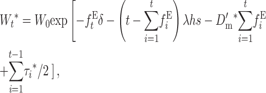or, using the accumulated inbreeding (),

Similarly, using Equation 26B for the average viability under NM, we obtain that EC gives larger average viability at generation t than NM when

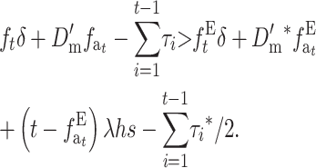(31A)

For N′ large enough that the equilibrium rate of deleterious fixation can be ignored, the condition for EC giving larger viability than NM reduces to

(31B)

The left side, δ(f_t − f_t^E), has a maximum for some intermediate f_t-value and then decreases to zero. On the contrary, () increases with t up to a limit, which is larger and takes longer to be attained for larger N′-values. Therefore, setting aside the effect of purging, this management strategy should be advantageous for the early generations during the shift. However, unless h-values are very small, EC will become disadvantageous as f_t^E approaches one. This disadvantage requires a relatively large N′-value to be important and will take a long time to emerge. Equations 31A and 31B also imply that this disadvantage will increase with increasing h-values, as these will produce small δ and large λhs. Note, however, that large λhs implies large (Equation 29); i.e., since the long-term disadvantage is due to a greater load from segregating deleterious mutations, it can be potentially recovered due to natural selection after NM is restored. As shown above, the long-term deleterious fixation rate (Equation 31A) is smaller under EC than under NM.

The purging term goes to zero as t increases, but it may be positive first and negative later, implying that delayed purging under EC can contribute to a middle-term advantage for this management strategy.

For N′ not too small, when both D_m and D_m′* can be neglected, Equation 30 reduces to the computationally more convenient expression

and

(32)

PREDICTIONS AND DISCUSSION

Checking the analytical predictions for the mutation–selection–drift balance:

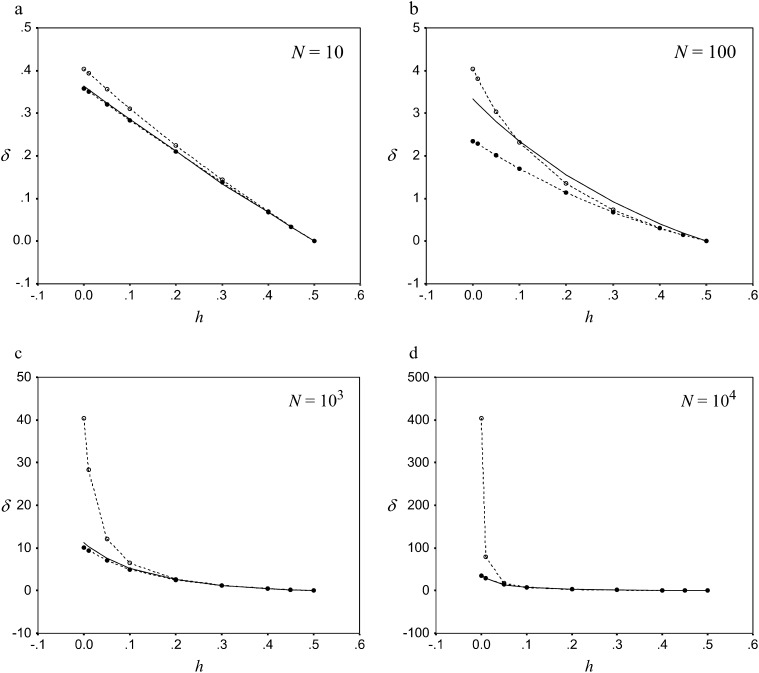
Figure 1 shows predictions for the inbreeding depression rate given by Equation 13 as a function of h, where s = 0.02 and different sections are for different population numbers. A prediction based just on the pervasiveness of the allele computed from its heterozygous effect (i.e., assuming K = 0) is given for comparison. It shows that the constraint on δ posed by selection against homozygous becomes highly relevant for h < 0.1 in large populations.

Figure 1.—

Equilibrium rates of inbreeding depression against the coefficient of dominance h. Diffusion predictions (solid line), Equation 13 predictions (dashed line with solid circles), and Equation 13 prediction assuming K = 0 (dashed line with open circles) are shown. In all cases s = 0.02 and λ = 1 for different effective population numbers: (a) N = 10, (b) N = 100, (c) N = 10³, and (d) N = 10⁴).

Predictions computed from diffusion theory are also given in Figure 1 and show that our approximation is excellent in most conditions. As an exception, our approach produces downwardly biased predictions for N = 100, suggesting that it overestimates the efficiency of natural selection when Ns = 2. This can be due to the inadequacy, in this case, of the assumption q ≪ p when accounting for natural selection (Equation 6). The predictions illustrate that the equilibrium inbreeding depression rate increases almost linearly with decreasing h-values for small populations. For large populations, however, δ becomes appreciable only for small h-values, and, then, selection against homozygous becomes a relevant limiting factor.

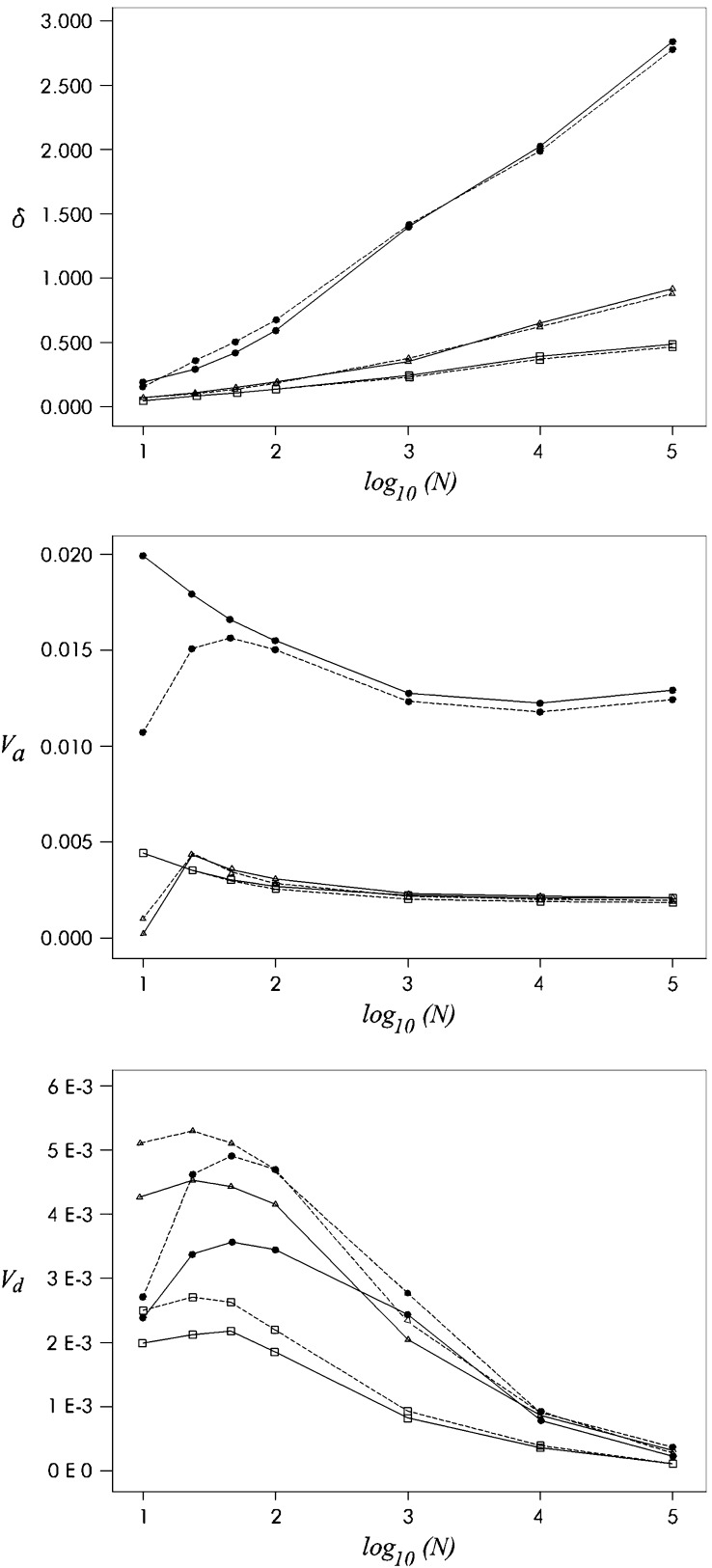
Figure 2 (top) gives predictions for the inbreeding depression rate obtained using either our approximation or the diffusion approach. Both are averaged over plausible distributions for mutational effects as in García-Dorado (2003).

Figure 2.—

Equilibrium genetic parameters for different mutational properties against log₁₀(N). Diffusion (solid line) and approximated (dashed line) predictions for the rate of inbreeding depression (δ, top), additive variance (V_a, middle), and dominant variance (V_d, bottom) against Log₁₀(N) for three different sets of mutational parameters are shown: (1) the “sensitive” S_c case, as in case c in Fernández and Caballero (2001) (solid circles), λ = 0.5, s exponentially distributed with average effect E(s) = 0.05, h uniformly distributed between 0 and exp[−ks] with average E(h) = 0.35; (2) the “tolerant” T_h case, as in case h in Fernández and Caballero (2001) (open squares), λ = 0.03, s gamma distributed with shape parameter 2.3 and average effect E(s) = 0.264, h uniformly distributed between 0 and exp[−ks] with average E(h) = 0.20; and (3) the “tolerant” T₁ case, as in García-Dorado (2003) (open triangles), λ = 0.03, s exponentially distributed with average effect E(s) = 0.224, h uniformly distributed between 0 and exp[−ks] with average E(h) = 0.20.

There has been extensive discussion of the rate of deleterious mutation and the corresponding effect distribution (García-Dorado et al. 2004). Basically, experiments by Mukai and co-workers with Drosophila melanogaster implied almost one deleterious mutation per new zygote, with average homozygous effect around a few percent, while later reanalysis and newer experiments gathered evidence that the rate of mutation with deleterious effect relevant in the context of this analysis is usually an order of magnitude below the one proposed by Mukai, with larger average homozygous effects on the order of 10⁻¹. Here I consider three mutational parameter sets, derived from Drosophila data, for which a more explicit justification can be found in García-Dorado (2003). One is a “sensitive” case (S_c) corresponding to the Mukai view, where fitness is mutationally sensitive, i.e., where most mutations have a relevant deleterious effect, although this is usually tiny or mild (the precise rates and effect distribution I use are those of model c in Fernández and Caballero 2001, to allow appropriate comparison to their simulation results). The other two are “tolerant” cases, where the deleterious effects of most mutations, although they may be large enough to constrain fixation probabilities in the evolutionary timescale, are too small to make a relevant contribution to the genetic properties studied here. In both tolerant cases, a small fraction of mutations have a mild to severe deleterious effect. One is the T₁ model in García-Dorado (2003), and the other one (T_h) is case h in Fernández and Caballero (2003), which is similar to T₁ with lower kurtosis for s.

Our approximations were averaged over 10⁴ mutations sampled from the corresponding joint distributions for s and h (see Figure 2 legend for mutational parameters). In general, they are in good agreement with the diffusion ones. This implies that mutations with small s- and h-values, for which our method gives downwardly biased δ-estimates, do not make a relevant contribution to the overall inbreeding depression rate, so that the approximation integrated over the distribution of mutational effects is highly reliable compared to the corresponding diffusion approximation (Figure 2, top). Figure 2 illustrates a δ-increase that is roughly linear on the decimal logarithm of the effective population number.

Figure 2 also gives predictions for additive (middle) and dominance (bottom) variances obtained from Equations 16 and 17, both averaged for the distributions corresponding to the different mutational parameters considered, together with the corresponding diffusion predictions (see above and Figure 2 legend). Additive variance approximations are excellent, except for small populations with S_c mutational parameters. This bias is due to the use of the approximation in Equation 16, where the rate of fitness decline from deleterious fixation in the new equilibrium (which is relevant in this particular case, see García-Dorado 2003) has been neglected. The reason is that, in this situation, mutations with very small effect, which can become fixed by drift in small populations, occur at a high rate. This bias could be corrected by using Equation 15.

The predictions for the dominance variance are reliable for large populations, but are overestimates for low to moderate size populations, the bias being important for the S_c case with N on the order of hundreds. This should again be ascribed to the inadequacy of the assumption q ≪ p (Equation 6) in this situation, where drift is relatively large.

Predictions for the additive variance and the mean for fitness during the shift process under no management:

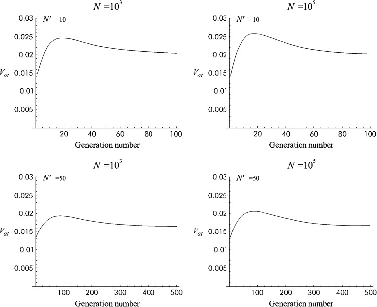
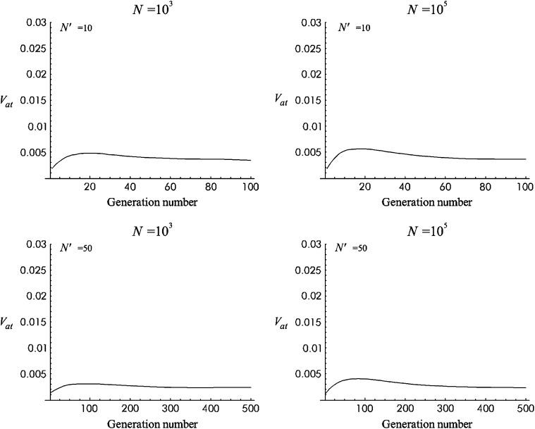
Figure 3 gives the predicted additive variance computed using this approximation for the S_c model (see parameter in Figure 2) for a 10N′ generation period after size reduction. Four situations, combining N = 10³ or 10⁵ and N′ = 10 or 50, are considered. Figure 4 is equivalent for T₁ mutational parameters. In all these cases, the additive variance reached a maximum value after ∼2N′ generations (f_t ≈ 0.64) and then decreased to approach a new balance with larger additive fitness variance. Under both models, the predicted increase in additive variance was higher for the larger ancestral population size (N = 10⁵) and for the more drastic size reduction (N′ = 10).

Figure 3.—

Additive variance with no management (NM) against generation number during 10N′ shift generations for S_c mutational parameters.

Figure 4.—

Additive variance for no management (NM) against generation number during 10N′ shift generations for T₁ mutational parameters.

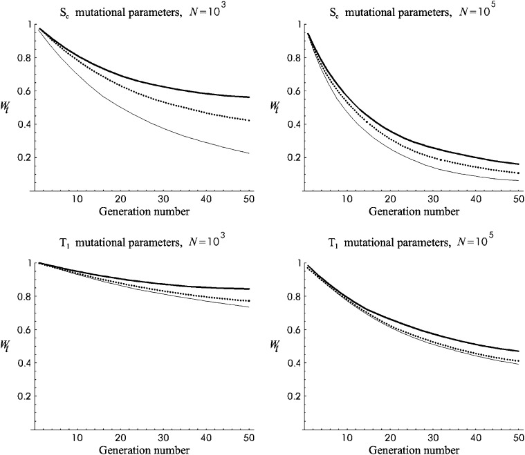
Figure 5 gives different predictions for average fitness through the first 50 shift generations under no management. Average fitness predicted using Equation 27 is considerably above the neutral expectation derived from the initial inbreeding depression rate (W_t = W₀ exp[−f_tδ]) and much higher than that including the mutational input of deleterious effects . The difference between these predictions is larger for S_c than for T₁ mutational parameters, as the former gives larger δ and larger mutational deleterious input.

Figure 5.—

Different predictions for the fitness average against generation number during the shift to a new balance for N′ = 25 under no management. Solid line, “shift approximations”; dotted line, predictions derived from the ancestral inbreeding depression rate δ; shaded line, predictions derived using δ and the mutational deleterious input.

Wang et al. (1999) obtained stochastic simulation results for N′ = 50 starting from a population at a recurrent mutation–selection balance with S_c-like mutational parameter {λ = 0.5, E(s) = 0.05, E(h) = 0.36, s exponentially distributed, h = exp[−ks]}. I obtained Equation 27 predictions for this case using ancestral genetic properties computed for the recurrent mutation model (δ and τ_t computed from Equations 1, 19, and 23, where q-values were computed from Equation 6.2.6. in Crow and Kimura 1970 for 5800 loci as in Wang et al. 1999). Our predictions are in good agreement with simulation results in their Table 2 up to generation 50 (differences <2%). From generation 50 to 100, however, the rate of viability decline in Wang et al. doubled, which is unexpected, particularly under the assumed multiplicative fitness model. On the contrary, our predictions indicate that, by generation 100, viability had recovered half of the previous decline. This difference can be partly ascribed to linkage in Wang et al.'s simulations, where the whole genome length is 2 M. As Wang et al. pointed out, associative overdominance induced by selection in the presence of linkage for h < 0.5 may reduce the effect of purging. Note that in the overdominant equilibrium the additive genetic variance is zero, so that associative overdominance, although it may induce considerable segregating load, should be expected to reduce additive variance in the long term and, therefore, to diminish the efficiency of purging. However, the above difference should also be partly a consequence of the use of Equation 27 (which neglects the fitness decay from deleterious fixation) instead of the analytically less tractable (26B) expression. This may become relevant in the long term (i.e., for high in Equation 26B), particularly for the S_c-like mutational parameter, for which D_m′ = 0.0016 for N′ = 50 (computed from diffusion theory).

Therefore, for small N′-values and S-like mutational parameters, (say N′ ∼ 10 and sensitive cases, see García-Dorado 2003), the rate of fitness decline from deleterious fixation becomes relevant, and using Equation 27 (instead of Equation 25 or its approximated expression in Equation 26B) may underestimate the long-term fitness decline.

EC vs. NM during the shift process under different mutational parameters:

We use Equations 27, 28, and 32 to predict the change in mean fertility or mean viability under NM or EC for different population numbers. In each case, predictions are averaged over 10⁴ (s, h)-values randomly sampled from the corresponding distribution, according to the mutational parameter (see Figure 2 legend).

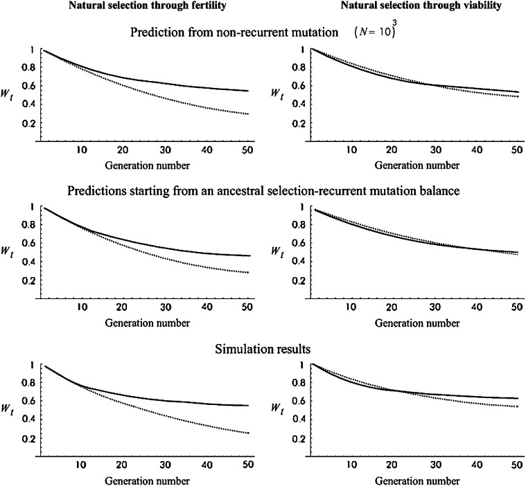
Figure 6 shows predictions for the cases simulated by Fernández and Caballero (2001) and given in their Figure 1, a–c. These refer to an ancestral population where 5800 loci segregate with the frequency expected at the balance between natural selection and recurrent mutation, as in Wang et al. (1999), but linkage was not considered in this case. S_c mutational parameters are used and Figure 6 gives the evolution of mean fitness when the effective population size is reduced to a stable value N′ = 25. I obtain predictions comparable to these simulation results following two different approaches.

Figure 6.—

Fitness average against generation number for the case simulated by Fernández and Caballero (2001): (50 shift generations for N′ = 25) predictions and simulation results. Solid lines, no management (NM); dotted lines, equal contribution (EC). Simulation results are from Fernández and Caballero (2001).

In Figure 6, top, I have used our predictions for nonrecurrent mutation assuming N = 1000. This N-value was chosen because it provides an ancestral inbreeding depression rate (δ = 1.49) very close to the value for nonrecurrent mutation in Fernández and Caballero's work (δ = 1.67). Furthermore, it also gives an equilibrium number of segregating loci (7383) that is of the order of that used in the simulation procedure. In Figure 6, middle, I have obtained predictions using ancestral genetic properties computed for the recurrent mutation model, with δ and τ_t computed from Equations 1 and 23, and using and with q-values obtained from Equation 6.2.6. in Crow and Kimura (1970) for 5800 loci, as for the Wang et al. (1999) case discussed above. Figure 6, bottom, gives Fernández and Caballero's simulation results. The left side compares results under NM and EC for natural selection acting on fertility, and the right side does the same for viability. The present shift approximations give quite precise fitness predictions for the EC-fertility case, where there is no selection, but NM and EC-viability predictions are downwardly biased by up to 10%. However, the good qualitative agreement between simulation and predictions in both cases is remarkable, indicating that, despite the approximations involved, our equations have considerable predictive power. A qualitative agreement was also found with transition matrix predictions by Schoen et al. (1998) and by Theodorou and Couvet (2003), although the absence of some details regarding the initial ancestral population and the distribution of h prevents formal comparison.

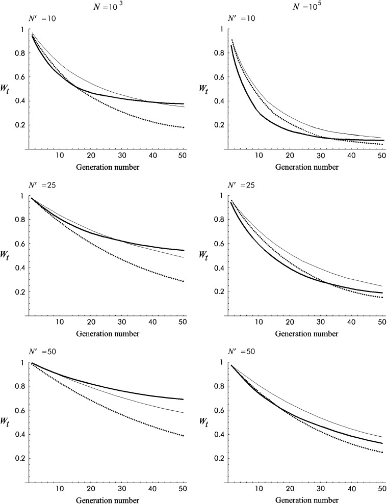
Figure 7 gives the evolution of fitness under S_c mutational parameters for NM and for fertility or viability under EC. Each section represents a different situation regarding N- and N′-values. For fertility, EC is at an advantage in the short term for large N- and small N′-values (cases with N/N′ ≳ 100), as this promotes large ancestral inbreeding depression rates and high inbreeding during the shift. Regarding viability, EC is always at an advantage for a considerable period if the ancestral population was large, but both the length of that period and the magnitude of the advantage become insignificant for smaller ancestral populations, unless the new size is very small.

Figure 7.—

Predictions for average fitness against generation number during shift from N to N′ for S_c mutational parameters. Solid line, no management (NM); dotted line, equal contribution (EC) when natural selection acts through fertility; thin line, equal contribution (EC) when selection acts through viability.

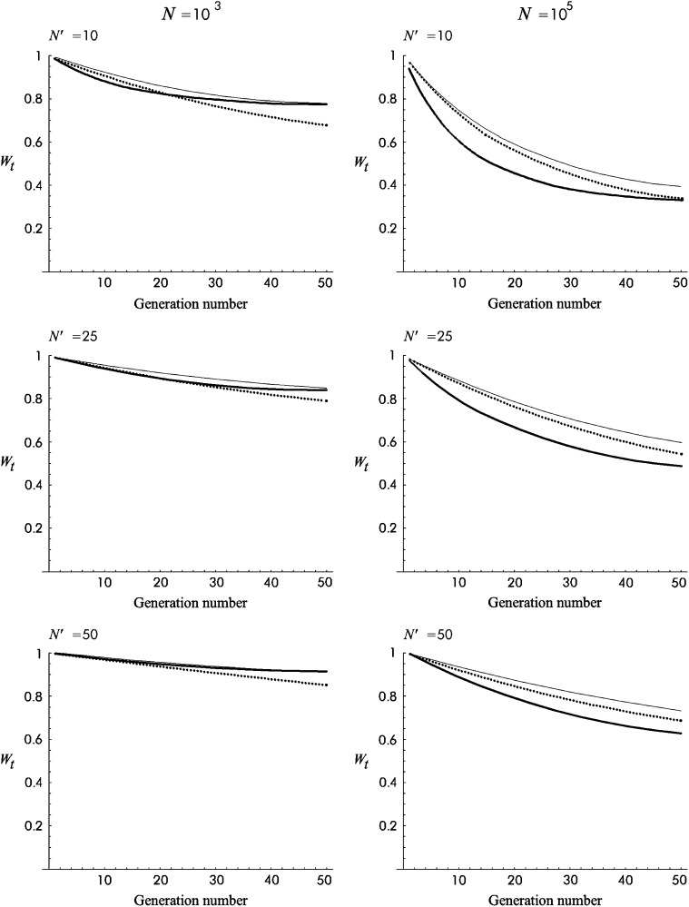
Figure 8 gives analogous results for T₁ mutational parameters. In this case, where the rate of relevant deleterious mutation is low and the average deleterious effect is moderate and predominantly recessive, EC is at an advantage for fertility in the short term for a larger spectrum of conditions (cases with N/N′ ≳ 40), because the additive variance is smaller and, therefore, purging is less efficient. Regarding viability, EC was always at some advantage during the period considered, although this was important only when the ancestral population was large.

Figure 8.—

Predictions for average fitness against generation number during shift from N to N′ for T₁ mutational parameters. Solid line, no management (NM); dotted line, equal contribution (EC) when selection acts through fertility; thin line, equal contribution (EC) when selection acts through viability.

Drosophila experimental studies have been performed to assess the advantage for EC strategies. Borlase et al. (1993) reported that, after 11 generations with N′ = 8, their population had relative fitness 0.123 if maintained with NM and 0.26 if EC was practiced. This is qualitatively consistent with our shift approximations, which predict in this case advantages of ∼0.1–0.2 for relative fertility and relative viability for all mutational parameter values considered above. Thus, using S_c mutational parameters with N = 10⁶ and N′ = 8, the approximation predicts relative fitness 0.14 after 11 generations with NM, while with EC it predicts 0.28 when selection acts through viability or 0.25 when it occurs through fertility. T models predict similar differences, but with higher fitness values (∼0.5 with EC). However, it is well known that inbreeding depression rates have considerable between-population variability, and recent results suggest that the rate of severely deleterious mutation with small h could be underestimated in mutation-accumulation experiments due to purging (García-Dorado et al. 2007). Thus, average deleterious effects could be slightly above those corresponding to T₁ parameters, leading to substantially higher inbreeding depression rates at equilibrium. As an ad hoc approximation, a T-like mutational parameter set with λ = 0.03, s exponentially distributed with average 0.3, and the same relationship between h and s as in the T₁ model, predicts for the Borlase et al. case (N = 10⁶, N′ = 8, t =11) relative fitness 0.26 under EC (both for viability and fertility) and 0.11 under NM. Thus, the Borlase et al. results are consistent with our predictions under a variety of mutational parameters, both for fertility and for viability.

Rodríguez-Ramilo et al. (2006) maintained Drosophila populations with N′ = 100 or 20 for 35 generations using NM or EC. In large populations, relative viability declined to ∼0.8, with no detectable difference between methods, while with N′ = 20, relative viability declined to ∼0.6, showing a small but consistent advantage for EC (see their Figure 5B). These results are qualitatively consistent with our approach assuming N = 10⁶ and T₁ mutational parameters, which predicts relative viability 0.90 under EC and 0.84 under NM for N′ = 100 and 0.69 under EC and 0.57 under NM for N′ = 20. The S_c mutational parameters predict a similar advantage pattern, but with too small average viability (∼0.55 for large populations and down to 0.11 for small ones).

Therefore, inspection of Figures 7 and 8, as well as empirical results, shows that EC is at an advantage regarding fitness for a wide range of situations, particularly if management is expected to be necessary for < ∼20 generations. However, analytical results and practical reasons make it convenient to separately consider fertility and viability. Thus, for relatively low N/N′ ratios, EC may convey a substantial disadvantage for fertility if detrimental mutations occur at a high rate, which is due to relaxed selection on fertility (Figure 7, left, for S_c mutational parameters). On the other hand, fertility traits might be prone to undergo adaptation to captive conditions, through modified breeding behavior, increased optimum litter sizes, etc., so that relaxed selection on fertility might become an additional advantage for EC management. In any case, it should be remembered that our conclusions refer just to direct effects on fitness and that an ancestral balance between deleterious mutation and drift is assumed and no forces other than these are considered during the process. Several mechanisms can lead to larger ancestral genetic variance and/or inbreeding depression rate for fitness, thus affecting the validity of the above predictions. Furthermore, for populations starting with high reproductive potential and good viability, other considerations, such as the improved maintenance of adaptive potential and variability or the slower rate of adaptation to captive conditions, may be more relevant when deciding on the advantages of using EC management.

APPENDIX A

Assuming Ns > 5, Li and Nei (1972) provide approximations for the whole expected number of heterozygous (n₁) and homozygous (n₂) individuals that will carry a new deleterious mutation while it will segregate in the population under two different assumptions (h > 0.3, h = 0, see below). Therefore, the ratio (where summation is over generations) can be computed as

This also gives the equilibrium ratio of the expected q²-value to the expected q-value at single generations. Thus, we compute

For h > 0.3, natural selection acts mainly through the mutant effect in the heterozygous state, so that n₁ = 1/hs and n₂ = 1/(8Nh²s²) (Equations 6b and 8b in Li and Nei 1972). Therefore, denoting by K_hs the K-value when hs > 0.3,

For h = 0, natural selection limits q-values only through selection against homozygous, and Li and Nei (1972, Equations 7b and 9c) give

and, denoting by K_s the K-value when h = 0,

We use

as a general approximation, where K is limited mainly by the more relevant deleterious effect (s or sh) in each case (i.e., the driving factor constraining is the homozygous deleterious effect when K_s ≪ K_hs and the heterozygous deleterious effect when K_hs ≪ K_s). This K approximation has been compared to values computed from diffusion approximation, showing a good behavior for quite general s-, h-, and N-values (results not shown). We note that when s goes to zero, K goes to , as is expected from diffusion theory.

APPENDIX B

The expected covariance cov_t(α², H) at any segregating locus between the squared average effect of a gene substitution (α = s/2 + (2q − 1)(1 − 2h)s/2, Falconer and Mackay 1996) and the corresponding heterozygosis in different populations randomly derived and maintained with effective size N′ from the ancestral population t generations ago can be written as cov_t(α², H) = [(s/2 + (2q − 1)(1 − 2h)s/2)², 2pq]. This gives

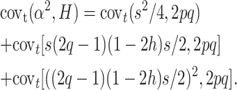Note that cov_t(s²/4, 2pq) = 0, and, for q ≪ p, cov_t[(2q − 1)², 2pq] ≈ cov_t[−4q, 2pq]. Furthermore, for q ≪ p, cov_t(q, 2pq) ≈ 2V_t(q), where V stands for variance. However, the last approximation ignores that, although for any q₀ ancestral q-value, by generation t we have E(q) = q₀, E(2pq) = 2p₀q₀(1 − f_t). To correct for this approximation we use cov_t(q, 2pq) ≈ 2(1 − f_t)V_t(q). As is well known, V_t(q) = pqf_t, so that, ignoring again quadratic q terms, pq ≈ q and

Therefore,

And, rearranging,

which, adding up over loci, gives

or

where

References

- Borlase, S. C., D. A. Loebel, R. Frankham, R. H. Nurthen, D. A. Briscoe et al., 1993. Modeling problems in conservation genetics using captive Drosophila populations: consequences of equalization of family sizes. Conserv. Biol. 7 122–131. [Google Scholar]
- Crow, J. F., 1979. Minor viability mutants in Drosophila. Genetics 92 s165–s172. [PubMed] [Google Scholar]
- Crow, J. F., and M. Kimura, 1970. An Introduction to Population Genetics Theory. Harper & Row, New York.
- Falconer, D. S., and T. Mackay, 1996. Introduction to Quantitative Genetics, Ed. 4. Longman, Essex, UK. [DOI] [PMC free article] [PubMed]
- Fernández, J., and A. Caballero, 2001. Accumulation of deleterious mutations and equalization of parental contributions in the conservation of genetic resources. Heredity 86 480–488. [DOI] [PubMed] [Google Scholar]
- Fisher, R. A., 1930. The Genetical Theory of Natural Selection. Clarendon Press, Oxford.
- Frankham, R., J. D. Ballou and D. A. Briscoe, 2002. Introduction to Conservation Genetics. Cambridge University Press, Cambridge, UK.
- García-Dorado, A., 2003. Tolerant versus sensitive genomes: the impact of deleterious mutation on fitness and conservation. Conserv. Genet. 4 311–324. [Google Scholar]
- García-Dorado, A., A. Caballero and J. F. Crow, 2003. On the persistence and pervasiveness of a new mutation. Evolution 57 2644–2646. [DOI] [PubMed] [Google Scholar]
- García-Dorado, A., C. López-Fanjul and A. Caballero, 2004. Rates and effects of deleterious mutations and their evolutionary consequences, pp. 20–32 in Evolution: From Molecules to Ecosystems, edited by A. Moya and E. Font. Oxford University Press, Oxford.
- García-Dorado, A., V. Ávila, E. Sánchez, A. Manrique and C. López-Fanjul, 2007. The buildup of mutation-selection-drift balance in laboratory Drosophila populations. Evolution Int. J. Org. Evolution 61 653–665. [DOI] [PubMed] [Google Scholar]
- Kimura, M., 1969. The number of heterozygous nucleotide sites maintained in a finite population due to steady flux of mutations. Genetics 61 893–903. [DOI] [PMC free article] [PubMed] [Google Scholar]
- Li, W. H., and M. Nei, 1972. Total number of individuals affected by a single deleterious mutation in a finite population. Am. J. Hum. Genet. 24 667–679. [PMC free article] [PubMed] [Google Scholar]
- López-Fanjul, C., A. Fernández and M.A. Toro, 2003. The effect of neutral nonadditive gene action on the quantitative index of population divergence. Genetics 164 1627–1633. [DOI] [PMC free article] [PubMed] [Google Scholar]
- Lynch, M., J. Conery and R. Bürger, 1995. Mutational meltdown in sexual population. Evolution 49 1067–1080. [DOI] [PubMed] [Google Scholar]
- Rodríguez-Ramilo, S. T., P. Moran and A. Caballero, 2006. Relaxation of selection with equalization of parental contributions in conservation programs: an experimental test with Drosophila melanogaster. Genetics 172 1043–1054. [DOI] [PMC free article] [PubMed] [Google Scholar]
- Schoen, D. J., J. L. Davis and T. M. Bataillon, 1998. Deleterious mutation accumulation and the regeneration of genetic resources. Proc. Natl. Acad. Sci. USA 95 394–399. [DOI] [PMC free article] [PubMed] [Google Scholar]
- Theodorou, K., and D. Couvet, 2003. Familial versus mass selection in small populations. Genet. Sel. Evol. 35 425–444. [DOI] [PMC free article] [PubMed] [Google Scholar]
- Wang, J., W. G. Hill, D. Charlesworth and B. Charlesworth, 1999. Dynamics of inbreeding depression due to deleterious mutations in small populations: mutations parameters and inbreeding rates. Genet. Res. 74 165–178. [DOI] [PubMed] [Google Scholar]
- Wright, S., 1938. Size of population and breeding structure in relation to evolution. Science 87 430–431. [Google Scholar]