Analysis of Kinetics in Noisy Systems: Application to Single Molecule Tethered Particle Motion

Abstract

In the tethered particle motion method the length of a DNA molecule is monitored by measuring the range of diffusion of a microsphere tethered to the surface of a microscope coverslip through the DNA molecule itself. Looping of DNA (induced by binding of a specific protein) can be detected with this method and the kinetics of the looping/unlooping processes can be measured at the single molecule level. The microsphere's position variance represents the experimental variable reporting on the polymer length. Therefore, data windowing is required to obtain position variance from raw position data. Due to the characteristic diffusion time of the microsphere, the low-pass filtering required to attain a good signal/noise ratio (S/N) in the discrimination of looped versus unlooped state impacts significantly the measurement's time resolution. Here we present a method for measuring lifetimes based on half-amplitude thresholding and then correcting the kinetic measurements, taking into account low S/N (leading to false events) and limited time resolution (leading to missed events). This method allows an accurate and unbiased estimation of the kinetic parameters under investigation, independently of the choice of the window used for variance calculation, with potential applications to other single molecule measurements with low S/N.

INTRODUCTION

The tethered particle motion method

Single molecule techniques have been first established in electrophysiology for the measurement of activity of single ion channels (1). These measurements have ever since represented a fundamental tool for the investigation of the kinetic properties of ion channels as well as of their mechanism of permeation and gating.

In the last decade, the single molecule approach has been extended to the study of many different enzymatic systems through the development of technologies apt to manipulate (2–6) and visualize (7), at the single molecule level, a variety of enzymes in the appropriate functional assays. Overcoming the limitations of bulk biochemical measurements, which sample the average signal from a very large (and often heterogeneous) population of molecules, these techniques allow the investigation of the reaction trajectory of a single enzyme, leading to an improved understanding of its biochemical mechanism and biophysical properties.

One single molecule technique is represented by the tethered particle motion method (TPM, (8–10)). In this method a biopolymer (typically a nucleic acid) is anchored at one end to the surface of a microscope coverslip and tagged at the other end with a microsphere. Thus, the microsphere is tethered to the glass surface through the polymer and exhibits a restricted Brownian diffusion with amplitude proportional to the length of the polymer itself. The range of diffusion can be measured with simple light microscopy techniques and can be used to detect variations in the length of the tether induced by the activity of structural or enzymatic proteins. This method, first developed for the study of the activity of RNA polymerase at the single molecule level (9,10), offers the great advantage of enabling biophysical and biochemical measurements at the single molecule level, yet requiring a very simple experimental apparatus. In addition to further studies on RNA polymerase (11,12), TPM has also been applied to the single molecule study of other proteins, including Lac repressor (8,13), and other systems (14–18).

Particularly interesting is the application of this method to the study of the dynamics of protein/DNA interaction, as in the case of Lac repressor (LacI): the binding of LacI simultaneously to two operators on the same DNA molecule induces the formation of a loop in the DNA molecule and alters its average end-to-end length. Therefore, the TPM signal can discriminate looped and unlooped state of the DNA molecule based on the amplitude of microsphere mobility switching between two discrete levels (8,13).

The kinetic analysis of single molecule data

As in single-channel measurements, a reliable and unbiased discrimination of the signal levels is needed for the determination of the dwell times of each state, which provides essential information on the kinetic and thermodynamic properties of the system under investigation. The methods for this type of analysis have been extensively developed for single-channel measurements. A large part of these approaches was first developed based on the use of a threshold for the discrimination between different ion conductance states (19). Because of instrumental band-pass and post-acquisition digital filtering of the data, these methods require corrections for the limited time resolution of the measurement (19–23). More recently, analysis methods based on fitting a kinetic scheme to the experimental data with a hidden-Markov algorithm (24–26) have become prevalent over threshold methods. In fact, the hidden-Markov methods provide great advantages in fitting even very complex kinetic schemes to experimental data. However, the experimental nature of the TPM measurement imposes a constraint which greatly limits the power of hidden-Markov due to the substantial difference between amplitude-based measurements (for example, patch-clamp) and variance-based measurements (for example, TPM). In a typical patch-clamp measurement, the experimental signal is represented by the current flowing through the patch, so that opening and closing of the channel is directly monitored by the alternation of a higher and a lower amplitude of the measured signal. In a typical TPM measurement, on the other hand, the position of the tethered microsphere is monitored in time and the experimental signal of interest (i.e., the signal reporting on the length of the DNA tether) is represented by the amplitude of motion of the microsphere, i.e., the variance of the measured microsphere position data. Different groups, through the years, have employed different parameters to quantify the amplitude of motion of the microsphere: the first method was based on averaging of the video images over a chosen time interval and calculation of an image-size parameter based on the measurement of the standard deviation of a Gaussian fit to the average image (8–11,14); subsequently, methods based on frame-by-frame measurement of bead position were adopted, either by measuring the standard deviation of position along one axis (15), or in the sample plane (13,17,18,27). Despite the methodological differences, in all cases, the quantity measured can be brought back to the concept of variance. This experimental condition determines a substantial difference with respect to the ion channel measurements (and all other methods also based on a direct measurement of changes in signal amplitude): in variance-based measurements, a time window has to be chosen, over which the signal variance will be measured, effectively imposing a low-pass filter to the data. Depending on the spectral characteristics of the noise and the signal/noise ratio (S/N), the choice of window can be very influential on the measured dwell times: generally, a wider window is more effective in reducing the noise and, thus, improving S/N but, at the same time, it will also reduce the time resolution in the filtered data, leading to loss of all the signal events that are short compared to the window width; this loss of events causes an overestimation of the measured dwell-times. On the other hand, a very narrow window will not cause loss of events, but will also not be effective in increasing S/N; the residual noise spikes will be able to cross the threshold and cause spurious events that fragment the true events, leading to an underestimation of the measured dwell-times. Therefore, an optimal filter is the one that offers the best tradeoff between S/N improvement and time resolution preservation. A similar experimental condition was encountered in the mechanical measurement of myosin activity with optical tweezers in the three-bead assay (28,29), where the relevant quantity is represented by the signal variance (the time-dependent amplitude of mobility of the trapped microsphere), rather than by the measured signal itself (the time-dependent position of the trapped microsphere). Smith et al. (29) developed a variance hidden-Markov method for the analysis of this type of optical tweezers measurements. This method requires the choice of an optimal window size for calculation of the variance; the choice is based on simulations and experimental measurements of the noise and signal properties (29). However, as described by the authors, the improvement of the variance hidden-Markov method over threshold methods is significant with S/N larger than ∼4. In some single molecule experiments (for example, TPM; single molecule FRET) this condition is not always satisfied, thus requiring the elaboration of an alternative approach for data analysis.

In the case of a low S/N, dwell-time analysis suffers not only from limited time resolution (due to low-pass filtering required to improve the discrimination between states, as indicated above), but also from the presence of false threshold crossings due to noise. An accurate determination of the lifetime of events measured with these methods, therefore, requires a full correction not only for missed events (false negatives due to low-pass filtering), but also for false positives.

The method for TPM kinetic analysis: application to Lac repressor

Here we present a general method for the kinetic analysis of noisy data obtained from a variance-based system switching between two variance levels. This method is demonstrated with an application to TPM data on LacI to extract quantitative information on the dwell times of the system independently of the window chosen for the variance measurement. The method is first developed simplifying the DNA-LacI system in the TPM experimental assay as a two-state system governed by first-order reaction rates in both directions. In the looped state (L), the LacI molecule binds simultaneously to the two operators on the DNA molecule: several lines of experimental evidence suggest that the TPM state with lower microsphere mobility has a 1:1 correspondence to the looped biochemical state (8,13). On the other hand, the TPM unlooped state (U) corresponds to a manifold of possible biochemical states (LacI not bound, LacI tetramer bound only to one operator, two different LacI tetramer molecules bound to the two operators, etc.). Our previous experimental work (13) allowed the description of the full scheme of the biochemical states underlying the TPM measurements on LacI, indicating that in each experimental condition adopted in the TPM experiment (mostly dependent on the LacI concentration) the unlooped state is dominated by two biochemical species at equilibrium. Thus, in this work we also extend the TPM data analysis method from the simple two-state system to this more complex and realistic representation of the experiment.

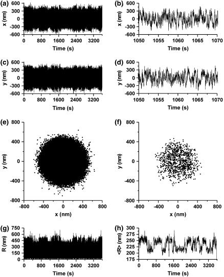
Fig. 1 shows a typical example of TPM data collected in a LacI experiment (for more details see Materials and Methods and Vanzi et al. (13)). The kinetic analysis of the system is based on the measurement of dwell times from traces such as that shown in Fig. 1 h. These data are obtained from the instantaneous measurements of microsphere position in the sample plane (R, Fig. 1 g) by convolution of the R(t) data with a normalized Gaussian function characterized by a standard deviation σ_g. This function represents the impulse response of what is commonly referred to as “Gaussian filter” (19), and the convolution described above is herein termed “Gaussian filtering” of the data.

FIGURE 1.

TPM experimental measurement. The position of the microsphere's centroid x (a shows the recording over 1 h, b shows, with an expanded timescale, a small section of the data to resolve details) and y (c shows the recording over 1 h, and d shows, with an expanded timescale, a small section of the data) coordinates are measured with a frequency of 50 Hz. (e,f) X-y scatter plots of the data displayed, respectively, in panels a, c and b, d. From the data shown in panels a and c, the instantaneous distance of the microsphere from the center of the distribution is calculated (R, g). (h) Data of panel g smoothed with a Gaussian filter with σ_g = 2 s (see text for more details).

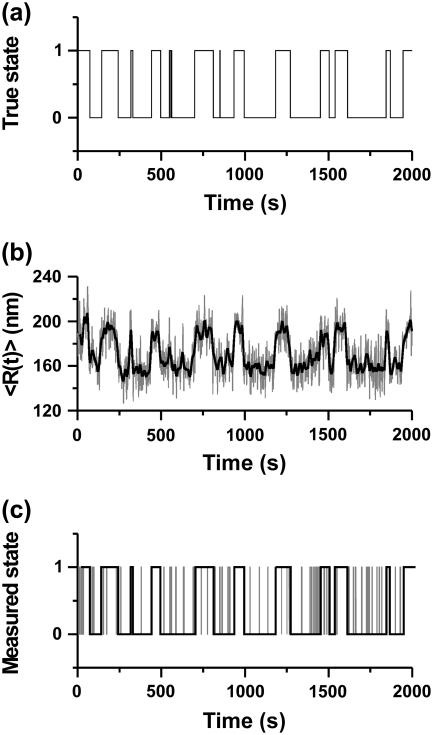
In our previous work we have experimentally demonstrated the quantitative effects of the choice of window (i.e., of the value of σ_g) on the looped and unlooped lifetimes measured by TPM (13). Fig. 2 illustrates the origin of these effects with an example. Transitions between the L and U states (Fig. 2 a) are associated with changes in the value of 〈R〉 (which is shown, for two different filters, in Fig. 2 b and represents the average mobility of the microsphere, i.e., the variance of the position signal measured in the sample plane over a chosen time interval, as illustrated in Fig. 1). Dwell time distributions and average lifetimes of L and U states can be measured by automated analysis of the 〈R〉 trace using the half-amplitude threshold method (19). When a threshold is set at half-amplitude between the two signal levels in a Gaussian-smoothed signal, true events shorter than a dead time T_d (corresponding to 1.35σ_g) are missed because they do not reach the threshold (19). Comparing the detected events (Fig. 2 c, shaded line, σ_g = 1 s and solid line, σ_g = 5 s) with the true data, which would be measured with infinite time resolution and no noise (shown in Fig. 2 a), it is evident that some events are missed (especially with σ_g = 5 s) because of limited time resolution in the filtered data. However, some false events are counted (especially with σ_g = 1 s) because of limited filtering, which leaves some residual noise capable of crossing the threshold. Missed events lead to an overestimation of dwell times, whereas false events lead both to an underestimation of dwell times and to the introduction of a spurious component (with the lifetime characteristic of the threshold-crossing false events) in the dwell time distributions. The lower limit to the time resolution of the measurement is set by the experimental apparatus (especially by the diffusion time of the microsphere, i.e., by the size of the microsphere itself). Additionally, the time resolution is decreased, and therefore the number of missed events increased, with low-pass filtering of the data that is required to increase the confidence in the discrimination between the two states. In contrast, filtering with a higher cutoff frequency (smaller σ_g) maintains higher time resolution, but increases the number of false events, due to the lower S/N attained.

FIGURE 2.

Effects of filtering on observed dwell times. Panel a shows an ideal trace with alternation between a looped state (L) and an unlooped state (U), switching between each other stochastically with an average lifetime of 50 s for both looped and unlooped state (see Materials and Methods for more details on the simulation). A TPM measurement of the system shown in panel a would lead to experimental data as those shown in panel b (shaded trace filtered with a Gaussian filter with σ_g = 1 s; black trace filtered with a Gaussian filter with σ_g = 5 s, see text for details). Panel c shows (with the same color coding as in b) the idealized traces obtained by analyzing the data in panel b with a half-amplitude threshold method.

Measurements relying on relatively high S/N (3–5 or higher, as in typical patch-clamp recordings) are characterized by a very low probability of false event detection (19), so that in the filtering and analysis of the signal, most attention has been devoted to the effects of missed events (19–22).

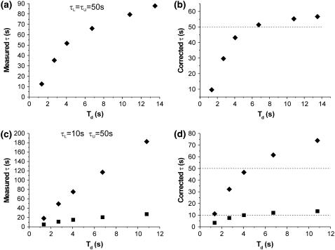
Fig. 3 shows an example of the dependence of the measured average looped and unlooped dwell times on the choice of σ_g, which determines the filter's dead time T_d. It is evident from the figure that there is a range of filters for which the effect of false events is dominant and the measured lifetimes grossly underestimate the real values. On the other hand, filtering with lower cutoff frequencies leads to a higher S/N, and therefore fewer false events, while the fraction of missed events increases, leading to an overestimate of the lifetimes. In the conditions of S/N typical of most TPM measurements, the curves of measured lifetimes display a continuity which does not warrant an intuitive choice of the right filter, if (as it is normal) the real values of the lifetimes are not known a priori. The corrections accounting exclusively for missed events (19,20) are most effective when filtering is sufficient to virtually reduce to zero the frequency of false events, while causing the loss of only a small fraction of true events. Fig. 3, a and b, demonstrates the effectiveness of one such method of correction (Eqs. 79 and 80 in Colquhoun and Sigworth (19)) when the true average lifetimes are very close in value: in this case, the corrected values tend to converge to a stable solution which is close to the true value. However, when the true average lifetimes are less similar to each other (as shown in the example of Fig. 3, c and d), or as the S/N of the measurements becomes smaller, these methods progressively fail (i.e., there is no convergence toward a unambiguous set of solutions) and corrections for the false events need to be also considered. The general method presented here takes into account both missed and false events and can be applied over a larger range of experimental conditions.

FIGURE 3.

Effect of filtering on measured lifetimes and correction for missed events. Simulated data characterized by τ_L and τ_U of 50 s (a, b) and 10 and 50 s, respectively (c, d) were filtered with different Gaussian filters (with the dead times, T_d, indicated, in each graph on the x-axis) and the measured average lifetimes were plotted versus filter's T_d (left panels). On the right panels the τ values obtained correcting for missed events only are plotted (squares for τ_L and diamonds for τ_U). (a, b) Only the values for measured and corrected τ_U were plotted for clarity, since those for τ_L overlapped.

The general concepts and mathematical corrections presented here can have a more general applicability to the analysis of noisy signals in different single molecule experiments and in other systems, in which hidden-Markov methods may not be applicable for a variety of reasons.

MATERIALS AND METHODS

The experimental TPM data acquisition and analysis

The experimental data collected in a typical TPM experiment are shown in Fig. 1. The apparatus and data collection have been described (13). Briefly, images of the microsphere are acquired at a frequency of 25 Hz and the centroid is calculated separately on the odd and even lines of each image, producing the x and y coordinates of the microsphere at a frequency of 50 Hz (an example is shown in Fig. 1, a–d). The radius of mobility of the microsphere is calculated as (see Fig. 1 g). From this, the signal variance (i.e., the average mobility of the microsphere in a given interval of time) is measured calculating 〈R(t)〉 by low-pass filtering the R(t) trace with a Gaussian filter. In this last step a choice on the averaging window size (29), corresponding to the standard deviation (σ_g) of the Gaussian filter's impulse response, must be operated. Fig. 1 h shows an example of 〈R(t)〉 calculated with σ_g = 2 s. From the 〈R(t)〉 data, the dwell times of the looped and unlooped states can be measured using, for example, a half-amplitude threshold (13,19).

Data simulations

To test the effectiveness of the correction methods presented below, we performed analysis on simulated data with known loop and unloop lifetimes and S/N properties similar to those of the TPM experimental data.

In this work we consider, at first, a two-state system (looped and unlooped DNA), in which the distribution of dwell times of each of the two states is exponential. For each chosen pair of average lifetimes (τ_L and τ_U), ideal recordings are generated as follows: the sampling rate of the recording is set to 50 Hz, as in the experimental recordings; when adding a point to the recording, a transition away from the present state (state i) is made if where Rnd is a double-precision floating-point random number between 0 and 1. An example of such an ideal recording is shown in Fig. 2 a for a τ_L and a τ_U of 50 s. As mentioned in the Introduction, in a typical TPM measurement the two states are discriminated based on the different range of microsphere mobility, i.e., based on the different variance or standard deviation in the signal of position of the microsphere. Simulated x(t) and y(t) data were generated by associating to the looped state a mean ± SD of 170 nm (both in x and y traces) and to the unlooped state a standard deviation of 220 nm, so to obtain simulated traces closely resembling the experimental data (these values of variances in the two states imply a S/N of <0.2 in the unfiltered R(t) trace). The noise imposed in these simulations is white in frequencies and Gaussian in amplitude distribution. The implications of this type of noise, as well as the assumptions adopted in the development of the correction methods below, are discussed in more detail in Appendix A.

The simulated traces were then analyzed following the same methods used for the analysis of experimental data (13).

Data were simulated with all permutations of τ_L and τ_U taking three possible values: 10 s, 50 s, and 100 s to reproduce lifetimes in a range similar to that of experimentally measured lifetimes (8,13). For each combination of τ_L and τ_U, 30 simulated traces (of the duration of 1 h each) were generated.

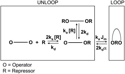
In the case of the more complete kinetic reaction scheme (shown in Fig. 4, see also (13)), the procedure followed to simulate the data was analogous, with the difference that three biochemical states (O-O, O-OR, and RO-OR) were all attributed to a unique TPM unlooped state. The rates of transitions between states (shown in Fig. 4) are defined in terms of the association and dissociation rate constants of LacI for a single operator (k_a and k_d, respectively). To provide a quantitative measurement of the effects of DNA bending energetics on the dynamics of loop formation, we introduced in the scheme the J_m factor commonly used in DNA circularization and looping (30,31). This factor describes the effective concentration of the free operator with respect to the other operator (bound to LacI), in full analogy with circularization experiments in which it is used to describe the effective concentration of one end of the circle with respect to the other (30,32). Several theoretical studies have described the dependence of J_m on the loop length and geometry (33), as well as on externally applied forces (33–35). The effects of loop strain on the rate of loop breakdown, on the other hand, have been shown to be negligible (8,13); however, for completeness (and possible applications to other systems) we introduce a phenomenological variable (α) that measures these effects (being 1 when there is no effect of strain, >1 when strain accelerates loop breakdown, and <1 when strain slows down loop breakdown, a quite unexpected case). Different sets of simulations (each set made of 30 simulated traces corresponding to 1 h of TPM recording each) were obtained varying, independently, J_m (between 10⁻⁸ M and 10⁻¹¹ M) and α (between 0.1 and 10). All simulations were run using home-written software in LABVIEW (v. 6.0, National Instruments, Austin, TX).

FIGURE 4.

Biochemical scheme of the reactions underlying the TPM measurements on Lac repressor-induced loop formation.

Development of the correction method

In this work we assume that the average and standard deviation of 〈R(t)〉 in the looped and unlooped states are known (the approach used to measure these properties of the TPM signal was described previously, (13)). Based on this knowledge and on the properties of Gaussian filters (19), we derive our method of data analysis.

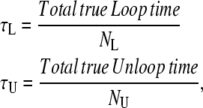
Considering two states (loop and unloop) both characterized by monoexponential distributions of dwell-times, the true average lifetime (τ) of each state (which, in the simple two-state model, corresponds to the reciprocal of the true rate constant for exit from that state) is simply described by

(1)

where N is the total number of events (loop or unloop as indicated by the subscript) in the true ideal recording.

Missed and false events affect both the total observed time in the two states and the number of transitions between them. If false and missed events could be characterized both in number and average duration, then the observed average lifetimes and number of observed events could be calculated as

(2)

(3)

(4)

(5)

where FL and FU are the numbers of false looped and unlooped states, respectively; ML and MU are the numbers of missed looped and unlooped states, respectively; and each τ represents the average lifetime of the false or missed events as indicated by the subscript.

In the TPM experiments, dwell-time analysis of the 〈R(t)〉 traces after half-amplitude thresholding produces a measurement of τ_Lo, τ_Uo, N_Lo, and N_Uo. To obtain the true values of τ_L, τ_U, N_L, and N_U from the above expressions, we need to calculate the values of FL, FU, ML, MU, τ_FL, τ_FU, τ_ML, and τ_MU as described point by point below.

Calculation of the number of false events

As mentioned above, the experimental TPM signal is smoothed with a Gaussian filter to obtain an 〈R(t)〉 trace on which the dwell times can be measured using the half-amplitude threshold method. When a threshold is chosen at a distance ϕ from the average amplitude of one state (which is, in turn, characterized by a Gaussian noise with standard deviation σ_n), the probability per unit time of threshold-crossing due to the noise has been calculated in the literature (19,36)

(6)

where f_c is the cutoff frequency of the Gaussian filter (corresponding to 0.1325/σ_g, (19)), k is a numerical factor that depends on the filter response and the noise spectrum and has a value of 0.849 for a Gaussian filter and white noise (19).

Here we will indicate with λ_FL and λ_FU the probability per unit time of generation of false loop and unloop events, respectively. Equation 6 allows calculation of the maximum number of false events as

(7)

and, similarly,

(8)

where σ_U and σ_L are the standard deviations of noise in the unlooped and looped state, respectively (false loop states are produced by threshold-crossings due to noise spikes originating from an unloop state, and vice versa). Equations 7 and 8 would allow exact calculation of the number of false events if no dynamic alternation between loop and unloop would occur. A demonstration of the validity of this expression for data with no U/L transitions, as well as a discussion on the assumption of the experimental noise in TPM being Gaussian and flat is provided in Appendix A.

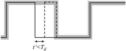
In the experimental situation, the calculation is complicated by the fact that the total time spent in each state (τ × N) is fragmented in N events rather than being continuous. Below we describe the effect of transitions between states on the observable number of false events, compared to the maximum theoretical number we just calculated in Eqs. 7 and 8. These effects are essentially due to the fact that an interval of time of duration T_d on each side of a state transition is not available for the generation of false events. In fact, false events that start within a time shorter than T_d from the previous true transition or end within a time shorter than T_d from the following true transition will not be picked out as false events. Instead, they will merge, respectively, with the previous or following true event, causing a distortion in the duration of those events but not a change in the number of transitions. If a false event is generated within a time t′ shorter than T_d after the previous true transition, the true transition and the on-transition of the false event are eliminated, since they delimit a state shorter than T_d. As a result of this, the false event is incorporated into the preceding true event, which is lengthened by the sum of duration of the false event and the time t′ (Fig. 5). The same effect takes place when a false event is followed by a true transition within a time t′ shorter than T_d.

FIGURE 5.

Effects of transitions on false events. The solid black line represents the real idealized data. The dotted line represents a false event due to crossing of the threshold by a noise spike. The thick shaded line represents the measured data obtained after half-amplitude threshold analysis applied with a filter characterized by a dead time T_d.

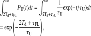
The effect described above can be summarized stating that the true unloop events that are shorter than 2T_d + τ_FL (where τ_FL is the average duration of the false loop events) cannot give rise to detectable false loop events; in fact, any false event occurring during one of these unlooped states would fall within the two cases described above. False loop events can, therefore, arise only during unlooped states longer than 2T_d + τ_FL. The fraction of these is simply given by

(9)

where P_U(t) is the true dwell-time probability distribution of the unloop state.

Thus, we obtain a corrected estimate of FL, after accounting for the fraction of unloop events too short to give raise to false loop events:

(10)

The same considerations can be symmetrically applied for the calculation of false unlooped states, obtaining:

(11)

Calculation of the duration of false events

The average duration of false looped and unlooped events due to threshold crossing by noise can be calculated based on an a priori knowledge of the standard deviation of the signal in each of the two TPM states. A similar problem has been solved for radar signals by Watts (37) based on the treatment of random noise by Rice (38). Filtering the TPM data (which is affected by noise approximated as white Gaussian noise) with a Gaussian filter (with standard deviation σ_g) imposes on the filtered signal the spectral properties of the filter itself (this point is demonstrated in Appendix A), so that the autocorrelation function of the filtered signal is

(12)

Following Watts (Eq. 7 in (37)), the duration (t_a) of a noise peak (with amplitude I) crossing the threshold (at distance φ from the average of the signal, as described above) is such that

(13)

and thus

(14)

so that

(15)

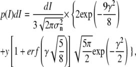
which describes the duration of the event as a function of I. The probability of a noise peak with amplitude I, on the other hand, is calculated following Rice (Eqs. 3.6–9 in (38)) as

(16)

where σ_n is the standard deviation of the noise in the state (looped or unlooped) from which the false threshold-crossing originates, erf represents the error function, and γ is defined as γ=I/σ_n.

Then, the average duration of the false events can be calculated as

(17)

with the known values of φ and σ_g, this integral is numerically solved using σ_L and σ_U in place of σ_n to calculate τ_FU and τ_FL, respectively.

Calculation of the number of missed events

Because of the limited time resolution of the filter, all events with a true duration of <T_d are missed altogether (19). Therefore the maximum number of missed loop and unloop events can be calculated as

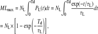(18)

and, similarly

(19)

Analogously to what was discussed above for false events, as an effect of the dynamic alternation of loop and unloop states and the limited time resolution, these numbers are decreased by the merging of adjacent states. Such merging will cause some events originally shorter than T_d to last longer than T_d in the filtered trace and, thus, not to be missed; this can take place according to two possibilities:

1. As illustrated above, an event can be lengthened by merging with a false event occurring within a time shorter than T_d from its boundaries, as shown in Fig. 5.

2. Similarly, if a short event is preceded by another true event (in the opposite state) which is missed, the two events merge and the short event in question should no longer be counted as missed.

We will now describe in detail the corrections to be introduced in the calculation of the number of missed loop events.

Point 1

We need to calculate the probability of false events that cannot be detected as such but instead merge with the adjacent true event. All false events originating within a true event with a duration comprised between T_d and 2T_d+τ_FL belong to this category, as discussed above. Also, within the true events with a longer duration, there is an interval of time corresponding to 2T_d+τ_FL partitioned at the two sides (the beginning and the end) of the event: false events taking place at these two edges of the transition will also fall within the category described at point 1. The total probability for these two conditions is given by

(20)

Point 2

The probability of an event as described at point 2 above is simply given by

(21)

For the correction of the number of missed events, we need to incorporate only events that do not fall in the categories calculated above, thus taking (1−P₁) and (1−P₂).

Combining these two corrections into Eq. 18 yields our estimate of the number of missed loop events:

(22)

And, similarly,

(23)

Calculation of the duration of missed events

Finally, the average duration of missed loop and unloop events can be simply calculated by

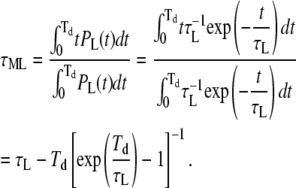(24)

And, similarly,

(25)

A more complex case: the kinetic scheme of TPM experiments on Lac repressor

The TPM measurements discriminate between the looped and unlooped state of the DNA molecule, offering a significant advantage over other biochemical or structural methods that do not distinguish directly if Lac repressor is bound to one or two operators (as in the case of filter binding assays, (39)) or reveal the presence of a loop but do not allow measurement of the kinetics of formation and disruption of such structure (as in the case of electron micrographs, (40)). However, the limitation of the TPM measurement consists in its inability to resolve between the different biochemical states that can be associated with the unlooped state (which are, potentially, up to nine, as discussed by the literature (8,41)). If we disregard the dissociation of the Lac repressor tetramer into dimers (42,43), a simplified scheme can be drawn for the biochemistry underlying the TPM experiments, as shown in Fig. 4. Based on the association and dissociation rate constants (k_a and k_d, respectively) measured for wild-type Lac repressor (39), which are also shown in the figure, at 100 pM LacI the two most populated biochemical states corresponding to the TPM unlooped state are the RO-O and RO-OR states. This is expected to give rise to a distribution of unloop dwell times which is no longer described by a single exponential (8,13). The two-state formalism developed above, therefore, needs to be improved taking into account the scheme shown in Fig. 4.

A similar biochemical scheme underlies single molecule fluorescence measurements on cholesterol oxidase (44). We solved the system of differential equations described by Lu et al. (44) imposing the initial condition U_RO-OR(0) = 0, U_O-OR(0) = 1, since every unloop state is initiated by a transition from the L to the O-OR state. A detailed description of this approach with explicit derivations is shown in Appendix B. This treatment leads to the following expression for the distribution of durations observed for the TPM unlooped state,

(26)

where a and b are defined as in Lu et al. (44),

(27)

(28)

and k₁, k₋₁, and k₂ are defined in terms of the rates indicated in Fig. 4 as follows: k₂ = J_mk_a; k₁ and k₋₁ are the rates of transition between O-OR and the other prevalent biochemical state corresponding to a TPM unloop (i.e., RO-OR at high LacI concentrations and O-O at low concentrations). So that, at the higher LacI concentrations (for example, 100 pM and 20 pM in (13)) k₁ corresponds to 2k_d and k₋₁ to k_a[LacI], while at lower concentrations (for example, 4 pM in (13)) k₁ corresponds to 2k_a[LacI] and k₋₁ to k_d. Repeating the calculations described in the previous sections using Eq. 26 for P_U(t) leads to the new set of correction equations for the full kinetic scheme. The equations are reported in Appendix B.

RESULTS

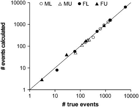
The expressions derived in the methods allow calculation of the number of events missed and created for any true couple of τ_L and τ_U and any chosen Gaussian filter, provided the knowledge of the signal amplitude and noise standard deviation in each measurable state. Using simulated data, we compared the numbers of missed and false events obtained by these calculations with those measured comparing the filtered data with the true data. An example of such a comparison is shown in Fig. 6. The data shown were obtained filtering with Gaussian filters with σ_g ranging between 1 s and 7 s. Fig. 6 demonstrates, with one example, the excellent agreement between the numbers of real and calculated missed and false events in these tests.

FIGURE 6.

Comparison between calculated and true values of ML, MU, FL, and FU. For a simulated data set with τ_L and τ_U equal to 10 s and 50 s, respectively, the values of missed and created events were calculated after filtering the data with Gaussian filters with σ_g of 1 s, 2 s, 3 s, 5 s, and 7 s. The calculated values are plotted against the true values obtained by comparing the true data with the data after filtering and idealization based on the half-amplitude threshold. The line represents a perfect correlation. The log-log scale was chosen to emphasize the good agreement of the calculated numbers with the true values over the large range of values of missed and created events involved with the array of filters used.

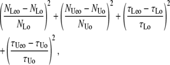
Knowing NL, NU, and the biochemical parameters (τ_L and τ_U in the case of the two-state system; k_a, k_d, α, and J_m in the case of the full biochemical scheme) as well as the signal's (φ, σ_L, σ_U) and filter's (T_d) properties, it is analytically possible to calculate, as described above, the values expected for ML, MU, FL, and FU (and, therefore, for τ_o and N_o for both loop and unloop). However, the reverse operation of calculation of true NL, NU, τ_L, and τ_U (or, NL, NU, α, and J_m in the case of the full biochemical scheme) values from the experimentally observed values of τ_Leo, τ_Ueo, N_Leo, and N_Ueo cannot be performed analytically. In comparison with the terms used in Eqs. 2–5 it should be noticed that we indicate the parameters experimentally observed with the subscript eo (these parameters are simply numbers, with their associated experimental uncertainties, provided by the measurements). The corresponding expressions for these parameters derived mathematically as a function of the true values of lifetimes and the properties of noise and filter, on the other hand, were indicated in Eqs. 2–5 with the subscript o, to emphasize that these expressions report the τ and N one would expect to observe, given a set of numerical values for the true lifetimes and the properties of noise and filter. Following a least-squares method as maximum likelihood estimator (45), the best estimates of true τ and N are those values of these variables that minimize the χ-squared expression

(29)

where, as discussed above, N_Lo, N_Uo, τ_Lo, and τ_Uo are defined in Eqs. 2–5, and N_Leo, N_Ueo, τ_Leo, and τ_Ueo are the experimentally measured values of these variables. The numerical minimization was implemented using the NMinimize function in Mathematica (v5.0, Wolfram Research, Champaign, IL), imposing the constraints that ML, MU, FL, and FU be ≥0. The numerical minimization in all cases leads to a stable, seemingly unique, solution within very large ranges of initial guesses.

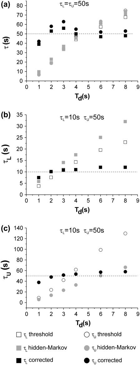
Fig. 7 shows examples of the results obtained for two cases: τ_L and τ_U both equal to 50 s (Fig. 7 a), and τ_L = 10 s, τ_U = 50 s (Fig. 7, b and c). The behavior of measured τ_L and τ_U versus filter chosen as well as the effectiveness of correcting only for missed events for these examples was shown in Fig. 3, where it was demonstrated (especially for the case of τ_L ≠ τ_U) that the corrections based solely on missed events are not adequate for the analysis of this type of data. In fact, especially in the case of τ_L and τ_U with significantly different values, correcting only for missed events does not lead to an unambiguous estimate of the true lifetimes, as the corrected values have a monotonic dependence on the chosen filter and do not tend to clearly asymptote to a stable value within a reasonable range of filters (Fig. 3 d). In Fig. 7 we also compare the effectiveness of our method with that of a hidden-Markov (HM) algorithm developed for the analysis of single molecule FRET data (46). The HM algorithm fails to lead to an unambiguous estimation of the τ-values. In fact, the effects of low-pass filtering the data to obtain the variance traces to be analyzed are not explicitly taken into account in current HM-based methods, which, in this situation, become merely a more sophisticated alternative to thresholding to obtain discrimination between the two TPM states, with no significant improvement in the estimation of the τ_L and τ_U.

FIGURE 7.

Comparison of threshold, hidden-Markov, and full correction methods. The lifetimes measured with the different methods are plotted in each graph as a function of the T_d of the filters used. (a) τ_L and τ_U are both 50 s. (b,c) τ_L = 10 s; τ_U = 50 s. (b) Values of τ_L; (c) values of τ_U. In the graphs the squares represent values measured for τ_L and the circles represent values measured for τ_U, using the half-amplitude threshold method (open symbols), the HM method (shaded symbols), and the method presented in this work (solid symbols).

It should be emphasized that this failure is not due to a limitation of the HM method per se. As discussed in the Introduction, and well detailed in Smith et al. (29), it is the fact that variance data is analyzed (rather than amplitude data) that compromises the possibility of using HM. Additionally, we should note that most of TPM data provides a S/N condition in which variance measurements must be operated with a range of window sizes encompassing time intervals comparable with those of the biological phenomena we are after. As discussed for the application of HM to the study of myosin (29), one must first determine (e.g., using simulations) the optimal size of the window for the variance calculation. In the application of HM to variance data, Smith et al. (29) also defined the conditions in which the method performs adequately, namely a S/N >∼4 and a large number of events in each experimental trace. The method proposed for the analysis of single molecule FRET data, on the other hand, performs very well even when these conditions break down (46). However, it is important to note that this method is applied to a signal directly measured as an amplitude change (in FRET efficiency), not requiring variance calculations, and thus, not suffering from all the low-pass-related issues discussed in this work.

Our method, on the other hand, is very stable over a large range of filters and allows an unbiased estimation of the true values of the lifetimes, which are indicated by the dotted lines in Fig. 7.

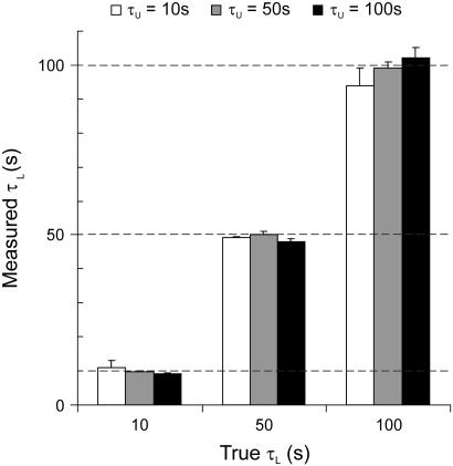
Fig. 8 summarizes results from the analysis of an array of simulated data with different combinations of τ_L and τ_U in a simple two-state system. The values of τ_L and τ_U were chosen in a range which is most significant for the expected lifetimes of looped and unlooped states in TPM measurements performed with wild-type and mutants of Lac repressor (13). In all the cases shown, the correspondence between the calculated values and the true values of the lifetimes was excellent (discrepancies were typically <5%, and in any case, <10%).

FIGURE 8.

Test of the correction method on a two-state system. The graph shows the lifetimes corrected with our method plotted versus the true lifetimes. A set of nine combinations of lifetimes for loop and unloop state between 10 s, 50 s, and 100 s was tested. The values plotted are the means obtained from all the filters applied to each trace (σ_g of 1 s, 2 s, 3 s, 5 s, and 7 s, as in Fig. 6). Error bars represent the mean ± SD.

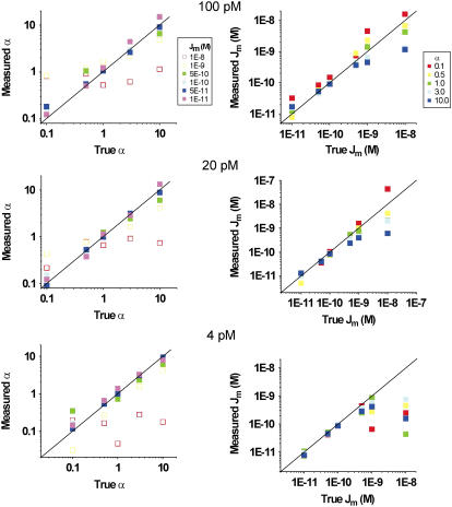
The more complex case, considering the full kinetic scheme of the LacI-DNA system in the experimental conditions of the TPM measurements, was also tested against data simulated at three different concentrations of LacI (4 pM, 20 pM, and 100 pM: the concentrations that were studied in the experimental work, (13)) and varying α and J_m in a range of two and three orders of magnitude, respectively. The ranges of these variables were chosen (from 0.1 to 10 for α; from 10⁻⁸ to 10⁻¹¹ for J_m) so to span all biologically relevant values and also to explore the limits of validity of both the analysis method and the TPM measurement in itself. Fig. 9 shows the results of these tests. Each plot compares the corrected value versus the true value of the variable considered (α, left panels; J_m, right panels). It can be noticed that, in all cases, the system fails to produce a correct estimation of α and J_m when the true J_m is >5 × 10⁻¹⁰. Such limit could be expected for the TPM technique simply considering the kinetics of the O-ORςORO reactions. With k_a = 6.2 × 10⁸ M⁻¹ s⁻¹ (39), a J_m of 10⁻⁹ M implies that loop formation from the O-OR state occurs at a rate of ∼0.6 s⁻¹. Most of the unloop events with an average lifetime of 1.7 s would, however, be missed due to the limited time resolution of the TPM experiments implemented with microspheres with a radius of few hundreds nanometers. In fact, in these conditions, filtering with a filter with T_d > 1.5–2 s is required to obtain a good discrimination between the looped and unlooped state. Thus, the measurement of J_m values above 5 × 10⁻¹⁰ M is not attainable with this technique. However, the approaching of this limit in the experimental measurements is clearly indicated by the corrected values of J_m leveling off (especially at the higher LacI concentrations) at values ∼5 × 10⁻¹⁰ M or slightly larger, as seen in Fig. 9. Thus, within the limits of validity imposed by the physical properties of microsphere diffusion in the TPM experiment, the correction method for the calculation of α and J_m proves valid through a range of values useful for measurements in many biological systems, including the LacI system.

FIGURE 9.

Test of the correction method on the full kinetic scheme of the TPM experiment. Correlation of the α (left panels) and J_m (right panels) parameters obtained with our correction method versus true values set in the data simulated for different LacI concentrations, as indicated above each set of panels (see text for description). The lines represent the perfect correlation.

DISCUSSION

The development of a variety of technologies capable of detecting and manipulating single molecules has extended the study of single molecule kinetics from the pioneering area of ion channels to many other enzymatic systems. These studies have led, in the last decade, to a much improved understanding of the biochemical and biophysical properties of many molecular motors, nucleic acid processing enzymes, and other biological systems. In the evolution of the patch-clamp techniques, in parallel with the technological improvements leading to higher S/N, a formidable attention has been devoted to the accuracy of the data analysis methods employed to obtain kinetic information from the experimental data. The patch-clamp measurements most often can rely on very high S/N and on the acquisition of experimental trajectories consisting of many hundreds or even thousands of events. These characteristics of the data allow a very effective implementation of HM algorithms. The HM algorithm can converge on a very stable fit to the data even when the kinetic model fitted is quite complex (i.e., implies several free fitting parameters) provided that the data is characterized by a very large number of events and a good S/N. HM has also been applied to laser tweezers data analysis (29): in this case the requirement of a large number of events is still fulfilled (traces of several seconds can be acquired while the characteristic times of actomyosin interactions are in the tens of milliseconds range), and S/N >3–5 can be attained.

In some cases, however, these criteria cannot be fulfilled. In the TPM experiment, typically measuring dynamics occurring on the scale of several tens of seconds, trajectories of 1–2 h are normally collected (longer traces are difficult to acquire because of both mechanical drifts in the experimental apparatus and a possible time-dependent loss of activity of the protein). In these conditions only a few tens of events can be observed in each recording. Furthermore, the TPM measurement is based on the thermal diffusion of the microsphere within the range limited by the tether, so that the confidence in the measurement of tether-length scales with the averaging time (10). When measuring dynamic processes by TPM, therefore, there is a trade-off between S/N (i.e., confidence in the loop/unloop discrimination, which is increased by low-pass filtering) and time resolution. Our characterization of the experimental system in a previous work has clearly illustrated this trade-off (13) and the need for an unbiased method for the estimation of the biologically relevant kinetic parameters. As mentioned in the previous sections, when uncorrelated measurements of the experimental variable can be obtained at rates much higher than the rates of transition between biochemical states in the system, then it is possible to reach a level of low-pass filtering at which the S/N attained is very high (i.e., the probability of generation of false events is made negligible), while the loss of information due to limitation of the measurement time resolution is not excessive. In these conditions, correction methods based on the calculation of missed events can be employed (19–21). Fig. 3 shows that these methods can have some effectiveness even for TPM measurements, provided that the lifetimes of the two biochemical states underlying the measurements are very similar and fairly long compared with the characteristic time of diffusion of the microsphere. When, on the other hand, these lifetimes are very different from each other, and at least one of them is close to the diffusion time of the microsphere, the correction only for missed events fails to produce an unambiguous estimate of the lifetimes. In fact, in these conditions, for any choice of filter, the lifetime of the longer state tends to be affected mostly by residual false events, while the lifetime of the shorter state is affected by missed events. Filters that virtually eliminate residual false events in the longer state would cause loss of the majority of the events in the short state, thus rendering the measurement unreliable. In this situation, the experimenter is forced to analyze data affected by both missed and false events. The methods presented in this work allow application of the required corrections in the case of a two-state system, as well as in the more complex case of the TPM measurements on LacI. In general, the same method can be extended to any biochemical scheme, provided that the measurable variable switches between two states and the duration probability distribution for each state can be explicitly calculated. Also, other experimental systems (both based on single molecule approaches or not) with similar properties (i.e., variance-based measurements and low S/N) can benefit from the approach described here for the measurement of dynamics to be extracted from a variance signal switching between two discrete levels.

APPENDIX A: VALIDATION OF ASSUMPTIONS ON TPM EXPERIMENTAL NOISE

All correction methods developed herein apply to data obtained after Gaussian smoothing of the raw experimental data as described in the Introduction and in the Materials and Methods (see also Fig. 1 in the main text). Therefore, in this context, we refer to the noise that is residual in the smoothed 〈R(t)〉 traces (see Fig. 1 h).

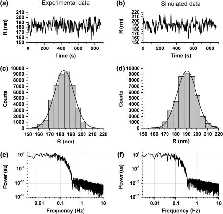
The correction methods developed in this work rest on the key assumption that the noise has Gaussian-distributed amplitude. Fig. 10 a shows an example of experimental data acquired in the presence of 100 pM LacI + 1 mM IPTG; Fig. 10 b shows an example of data simulated for a system which is stationary in the unlooped state. Fig. 10, c and d, shows the amplitude distributions of the 〈R〉 data. The figures demonstrate Gaussian distributions in the noise, confirming that this key assumption is indeed respected by the data. In Fig. 10 we show the behavior of simulated and experimental data in the absence of U/L transitions for clarity and for the following discussion on time-domain effects. However, in our previous experimental work (13) we demonstrated that the filtered experimental 〈R〉 data is characterized by noise with Gaussian-distributed amplitude also in the presence of U/L transitions.

FIGURE 10.

Amplitude and time correlation of noise. (a) Experimental recording acquired in the presence of 100 pM LacI + 1 mM IPTG. (b) Data simulated for a system stationary in the unloop state. For both panels, data filtered with σ_G=2 s was chosen. (c, d) Amplitude distributions for the data in panels a and b, respectively. The solid line represents a Gaussian fit to the data, using the function The best fit parameters were as follows: (c) A = 9874, R₀ = 183.6, σ = 18.9; (d) A = 9491, R₀ = 190.6, σ = 18.1. (e, f) Power spectra of the data shown in panels a and b, respectively.

With regard to the time correlation properties of the noise, we observe that, in the conditions of the TPM experiment, the spectral properties of the noise are in large part determined by the properties of the Gaussian filter.

The raw position data (an example is shown in Fig. 1) display an autocorrelation exponentially decaying with a time constant of 60–100 ms (data not shown), due to the diffusive properties of the microsphere. Thus, the physics of the TPM system indeed does not warrant a white (or time-uncorrelated) noise in the experimental measurements. However, below we demonstrate that even starting from an ideal white noise (as in the case of simulated data), Gaussian filtering imposes to the filtered data a power spectrum largely dominated by the properties of the filter. In fact, it can be noticed that the spectral properties of the filtered simulated data (Fig. 10 f) are indistinguishable from those of the filtered experimental data (Fig. 10 e). Thus, for the purposes of validation of our method, the simulated data is perfectly adequate.

Furthermore, that the assumptions made on the properties of the noise are indeed respected by the experimental data is demonstrated by calculating the number of false events expected according to Eq. 7 in traces obtained in the presence of 100 pM LacI + 1 mM IPTG (or in the absence of LacI altogether), when the system is trapped in the unlooped state. The numbers calculated can be compared with the number of transitions measured in those experimental traces, which are entirely due to threshold-crossing due to noise. The results of this comparison show an excellent agreement between calculated and measured values, as presented in Table 1.

TABLE 1.

Comparison of calculated and measured threshold crossings due to noise

σg (s)	σU (nm)	φ (nm)	FL measured	FL calculated
1	11.40	14.5	48	44
		6.2	80	86
2	8.64	14.5	11	12
		6.2	36	38
3	7.35	14.5	4	5
		6.2	22	23
4	6.04	14.5	2	1
		6.2	18	15

An experimental trace acquired in the presence of 100 pM LacI + 1 mM IPTG was filtered with Gaussian filters with four values of σ_g. The column labeled with σ_U reports the standard deviation of 〈R〉 in the filtered trace. The number of transitions occurring across a threshold imposed at a distance φ (indicated in the third column) from the average value of 〈R〉 was measured (FL measured) for two different values of φ. The number of transitions expected on ideal data respecting all assumptions done in this work was calculated following Eq. 7 in the main text and is reported in column labeled FL calculated.

APPENDIX B: CALCULATION OF UNLOOP DWELL TIME DISTRIBUTION FOR FULL KINETIC SCHEME

In the main text we have derived the mathematical expressions describing the number of missed events (false negatives due to low-pass filtering of the data) and false events (false positives due to threshold-crossing by residual noise in the filtered data). These expressions explicitly depend on the properties of the filter (namely its dead time, T_d), on the threshold chosen, on the noise, and on the expected shape of the dwell-time distributions. In particular, the expressions in the main text were derived for a two-state system, characterized by a monoexponential distribution of dwell-times for both the looped and unlooped states. As described in the Introduction, schematically shown in Fig. 4, and discussed in more detail in Vanzi et al. (13), however, the TPM experiment on LacI is more complex. In fact, experimental data (8,13) show that the dwell-time distribution for the unlooped sate is at least bi-exponential. Based on this observation, and on the experimental evidence suggesting that, in the conditions adopted in our measurements, LacI is predominantly in the tetrameric form (42,43), we describe the full kinetic scheme of the reactions underlying the TPM experiment as shown in Fig. 4. Based on this scheme we still expect a monoexponential distribution of dwell-times for the looped state (decaying with a characteristic lifetime of (2αk_d)⁻¹), whereas the distribution of dwell-times for the unlooped state (which, in the TPM experiment is the sum of the O-O, O-OR, and RO-OR states) becomes more complex. The calculation of a dwell-time distribution deriving from single molecule measurements lumping in one apparent state two biochemical states has been developed by Lu et al. (44) for experiments on cholesterol oxidase. In that experiment, the fluorescence from flavin adenine dinucleotide (FAD) was monitored. FAD (the oxidized form of the dinucleotide) is fluorescent, whereas FADH₂ (the reduced form) is not. The Michaelis-Menten classical enzyme kinetics for the reaction

(A1)

(where S is the cholesterol substrate and E is the enzyme) was used to calculate the distribution of dwell-times for the on-state (E-FAD, with or without S bound).

Following this example, we elaborated the equations for our scheme (Fig. 4), under the assumption that the TPM unlooped state is due to the sum of the O-OR state and either the RO-OR or the O-O state, depending on the conditions of the experiment. In fact, when k_a[R] ≫ k_d (which is the case at 100 pM LacI concentration) RO-OR is prevalent over O-O, and when k_a[R] ≪ k_d (which is the case at 4 pM LacI concentration), O-O is prevalent over RO-OR. Thus we write the following reaction path

(A2)

(where U₂ is always the O-OR state and U₁ is either RO-OR or O-O, as discussed above).

We can then write the equations governing the time-dependent probabilities of finding the system in each of these three states:

(A3)

(A4)

(A5)

This set of differential equations is solved using the Laplace transform with the initial conditions U₁(0) = 0, and U₂(0) = 1, which derives from the fact that, in the TPM experiment, the observed Loop → Unloop transition always leads into the U₂ state. The solution found is

(A6)

where

(A7)

(A8)

The probability of the system making a transition U₂ → L (i.e., ending the TPM unlooped state) is given by k₂U₂. Therefore P_U(t) = k₂U₂(t), leading to Eq. 26 in the text.

Thus, all mathematical relationships derived with the involvement of P_U(t) (i.e., FL, ML, MU, τ_MU, τ_Uo) need to be recalculated using this more complete expression for P_U(t), leading to the following results:

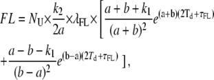(A9)

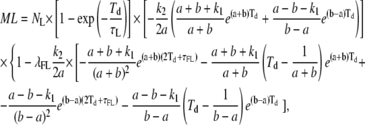(A10)

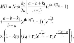(A11)

(A12)

(A13)

References

- 1.Neher, E., and B. Sakmann. 1976. Single-channel currents recorded from membrane of denervated frog muscle fibers. Nature. 260:799–802.1083489 [Google Scholar]
- 2.Bustamante, C., J. C. Macosko, and G. J. Wuite. 2000. Grabbing the cat by the tail: manipulating molecules one by one. Nat. Rev. Mol. Cell Biol. 1:130–136. [DOI] [PubMed] [Google Scholar]
- 3.Mehta, A. D., M. Rief, J. A. Spudich, D. A. Smith, and R. M. Simmons. 1999. Single-molecule biomechanics with optical methods. Science. 283:1689–1695. [DOI] [PubMed] [Google Scholar]
- 4.Capitanio, M., F. Vanzi, C. Broggio, R. Cicchi, D. Normanno, G. Romano, L. Sacconi, and F. S. Pavone. 2004. Exploring molecular motors and switches at the single-molecule level. Microsc. Res. Tech. 65:194–204. [DOI] [PubMed] [Google Scholar]
- 5.Allemand, J. F., D. Bensimon, and V. Croquette. 2003. Stretching DNA and RNA to probe their interactions with proteins. Curr. Opin. Struct. Biol. 13:266–274. [DOI] [PubMed] [Google Scholar]
- 6.Strick, T., J. Allemand, V. Croquette, and D. Bensimon. 2000. Twisting and stretching single DNA molecules. Prog. Biophys. Mol. Biol. 74:115–140. [DOI] [PubMed] [Google Scholar]
- 7.Ishijima, A., and T. Yanagida. 2001. Single molecule nanobioscience. Trends Biochem. Sci. 26:438–444. [DOI] [PubMed] [Google Scholar]
- 8.Finzi, L., and J. Gelles. 1995. Measurement of lactose repressor-mediated loop formation and breakdown in single DNA molecules. Science. 267:378–380. [DOI] [PubMed] [Google Scholar]
- 9.Schafer, D. A., J. Gelles, M. P. Sheetz, and R. Landick. 1991. Transcription by single molecules of RNA polymerase observed by light microscopy. Nature. 352:444–448. [DOI] [PubMed] [Google Scholar]
- 10.Yin, H., R. Landick, and J. Gelles. 1994. Tethered particle motion method for studying transcript elongation by a single RNA polymerase molecule. Biophys. J. 67:2468–2478. [DOI] [PMC free article] [PubMed] [Google Scholar]
- 11.Tolic-Norrelykke, S. F., A. M. Engh, R. Landick, and J. Gelles. 2004. Diversity in the rates of transcript elongation by single RNA polymerase molecules. J. Biol. Chem. 279:3292–3299. [DOI] [PubMed] [Google Scholar]
- 12.Yin, H., I. Artsimovitch, R. Landick, and J. Gelles. 1999. Nonequilibrium mechanism of transcription termination from observations of single RNA polymerase molecules. Proc. Natl. Acad. Sci. USA. 96:13124–13129. [DOI] [PMC free article] [PubMed] [Google Scholar]
- 13.Vanzi, F., C. Broggio, L. Sacconi, and F. S. Pavone. 2006. Lac repressor hinge flexibility and DNA looping: single molecule kinetics by tethered particle motion. Nucleic Acids Res. 34:3409–3420. [DOI] [PMC free article] [PubMed] [Google Scholar]
- 14.Dohoney, K. M., and J. Gelles. 2001. Chi-sequence recognition and DNA translocation by single RecBCD helicase/nuclease molecules. Nature. 409:370–374. [DOI] [PubMed] [Google Scholar]
- 15.Pouget, N., C. Dennis, C. Turlan, M. Grigoriev, M. Chandler, and L. Salome. 2004. Single-particle tracking for DNA tether length monitoring. Nucleic Acids Res. 32:e73. [DOI] [PMC free article] [PubMed] [Google Scholar]
- 16.Tolic-Norrelykke, S. F., M. B. Rasmussen, F. S. Pavone, K. Berg-Sorensen, and L. B. Oddershede. 2006. Stepwise bending of DNA by a single TATA-box binding protein. Biophys. J. 90:3694–3703. [DOI] [PMC free article] [PubMed] [Google Scholar]
- 17.van den Broek, B., F. Vanzi, D. Normanno, F. S. Pavone, and G. J. Wuite. 2006. Real-time observation of DNA looping dynamics of Type IIE restriction enzymes NaeI and NarI. Nucleic Acids Res. 34:167–174. [DOI] [PMC free article] [PubMed] [Google Scholar]
- 18.Vanzi, F., S. Vladimirov, C. R. Knudsen, Y. E. Goldman, and B. S. Cooperman. 2003. Protein synthesis by single ribosomes. RNA. 9:1174–1179. [DOI] [PMC free article] [PubMed] [Google Scholar]
- 19.Colquhoun, D., and F. J. Sigworth. 1983. Fitting and statistical analysis of single-channel records. In Single-Channel Recording. B. Sakmann and E. Neher, editors. Plenum Press, New York.
- 20.Blatz, A. L., and K. L. Magleby. 1986. Correcting single channel data for missed events. Biophys. J. 49:967–980. [DOI] [PMC free article] [PubMed] [Google Scholar]
- 21.Magleby, K. L., and D. S. Weiss. 1990. Estimating kinetic parameters for single channels with simulation. A general method that resolves the missed event problem and accounts for noise. Biophys. J. 58:1411–1426. [DOI] [PMC free article] [PubMed] [Google Scholar]
- 22.Roux, B., and R. Sauve. 1985. A general solution to the time interval omission problem applied to single channel analysis. Biophys. J. 48:149–158. [DOI] [PMC free article] [PubMed] [Google Scholar]
- 23.Qin, F., A. Auerbach, and F. Sachs. 1996. Estimating single-channel kinetic parameters from idealized patch-clamp data containing missed events. Biophys. J. 70:264–280. [DOI] [PMC free article] [PubMed] [Google Scholar]
- 24.Chung, S. H., J. B. Moore, L. G. Xia, L. S. Premkumar, and P. W. Gage. 1990. Characterization of single channel currents using digital signal processing techniques based on hidden Markov models. Philos. Trans. R. Soc. Lond. B Biol. Sci. 329:265–285. [DOI] [PubMed] [Google Scholar]
- 25.Qin, F., A. Auerbach, and F. Sachs. 2000. Hidden Markov modeling for single channel kinetics with filtering and correlated noise. Biophys. J. 79:1928–1944. [DOI] [PMC free article] [PubMed] [Google Scholar]
- 26.Qin, F., A. Auerbach, and F. Sachs. 2000. A direct optimization approach to hidden Markov modeling for single channel kinetics. Biophys. J. 79:1915–1927. [DOI] [PMC free article] [PubMed] [Google Scholar]
- 27.Pouget, N., C. Turlan, N. Destainville, L. Salome, and M. Chandler. 2006. IS911 transpososome assembly as analyzed by tethered particle motion. Nucleic Acids Res. 34:4313–4323. [DOI] [PMC free article] [PubMed] [Google Scholar]
- 28.Finer, J. T., R. M. Simmons, and J. A. Spudich. 1994. Single myosin molecule mechanics: picoNewton forces and nanometer steps. Nature. 368:113–119. [DOI] [PubMed] [Google Scholar]
- 29.Smith, D. A., W. Steffen, R. M. Simmons, and J. Sleep. 2001. Hidden-Markov methods for the analysis of single-molecule actomyosin displacement data: the variance-hidden-Markov method. Biophys. J. 81:2795–2816. [DOI] [PMC free article] [PubMed] [Google Scholar]
- 30.Shore, D., J. Langowski, and R. L. Baldwin. 1981. DNA flexibility studied by covalent closure of short fragments into circles. Proc. Natl. Acad. Sci. USA. 78:4833–4837. [DOI] [PMC free article] [PubMed] [Google Scholar]
- 31.Yamakawa, H., and W. H. Stockmayer. 1972. Statistical mechanics of wormlike chains. II. Excluded volume effects. J. Chem. Phys. 57:2843–2854. [Google Scholar]
- 32.Shore, D., and R. L. Baldwin. 1983. Energetics of DNA twisting. I. Relation between twist and cyclization probability. J. Mol. Biol. 170:957–981. [DOI] [PubMed] [Google Scholar]
- 33.Yan, J., R. Kawamura, and J. F. Marko. 2005. Statistics of loop formation along double helix DNAs. Phys. Rev. E Stat. Nonlin. Soft Matter Phys. 71:061905. [DOI] [PubMed] [Google Scholar]
- 34.Blumberg, S., A. V. Tkachenko, and J. C. Meiners. 2005. Disruption of protein-mediated DNA looping by tension in the substrate DNA. Biophys. J. 88:1692–1701. [DOI] [PMC free article] [PubMed] [Google Scholar]
- 35.Sankararaman, S., and J. F. Marko. 2005. Formation of loops in DNA under tension. Phys. Rev. E Stat. Nonlin. Soft Matter Phys. 71:021911. [DOI] [PubMed] [Google Scholar]
- 36.Papoulis, A. 1965. Probability, Random Variables and Stochastic Processes. McGraw-Hill, New York.
- 37.Watts, S. 1999. Duration of radar false alarms in band-limited Gaussian noise. IEE Proc. Radar, Sonar Navig. 146:273–277. [Google Scholar]
- 38.Rice, S. O. 1945. Mathematical analysis of random noise. Bell. Syst. Tech. J. 24:46–156. [Google Scholar]
- 39.Hsieh, W. T., P. A. Whitson, K. S. Matthews, and R. D. Wells. 1987. Influence of sequence and distance between two operators on interaction with the lac repressor. J. Biol. Chem. 262:14583–14591. [PubMed] [Google Scholar]
- 40.Kramer, H., M. Niemoller, M. Amouyal, B. Revet, B. von Wilcken-Bergmann, and B. Muller-Hill. 1987. lac repressor forms loops with linear DNA carrying two suitably spaced lac operators. EMBO J. 6:1481–1491. [DOI] [PMC free article] [PubMed] [Google Scholar]
- 41.Brenowitz, M., A. Pickar, and E. Jamison. 1991. Stability of a Lac repressor mediated “looped complex”. Biochemistry. 30:5986–5998. [DOI] [PubMed] [Google Scholar]
- 42.Barry, J. K., and K. S. Matthews. 1999. Thermodynamic analysis of unfolding and dissociation in lactose repressor protein. Biochemistry. 38:6520–6528. [DOI] [PubMed] [Google Scholar]
- 43.Levandoski, M. M., O. V. Tsodikov, D. E. Frank, S. E. Melcher, R. M. Saecker, and M. T. Record, Jr. 1996. Cooperative and anticooperative effects in binding of the first and second plasmid Osym operators to a LacI tetramer: evidence for contributions of non-operator DNA binding by wrapping and looping. J. Mol. Biol. 260:697–717. [DOI] [PubMed] [Google Scholar]
- 44.Lu, H. P., L. Xun, and X. S. Xie. 1998. Single-molecule enzymatic dynamics. Science. 282:1877–1882. [DOI] [PubMed] [Google Scholar]
- 45.Press, W. H., S. A. Teukolsky, W. T. Vetterling, and B. P. Flannery. 1992. Numerical Recipes in C. The Art of Scientific Computing. Cambridge University Press, Cambridge, MA.
- 46.McKinney, S. A., C. Joo, and T. Ha. 2006. Analysis of single-molecule FRET trajectories using hidden Markov modeling. Biophys. J. 91:1941–1951. [DOI] [PMC free article] [PubMed] [Google Scholar]