

Abstract
The hypothetical scanning (HS) method is a general approach for calculating the absolute entropy, S, and free energy, F, by analyzing Boltzmann samples obtained by Monte Carlo (MC) or molecular dynamics (MD) techniques. With HS applied to a fluid, each configuration i of the sample is reconstructed by gradually placing the molecules in their positions at i using transition probabilities (TPs). With our recent version of HS, called HSMC-EV, each TP is calculated from MC simulations, where the simulated particles are excluded from the volume reconstructed in previous steps. In this paper we remove the excluded volume (EV) restriction, replacing it by a “free volume” (FV) approach. For liquid argon, HSMC-FV leads to an improvement in efficiency over HSMC-EV by a factor of 2–3. Importantly, the FV treatment greatly simplifies the HS implementation for liquids, allowing a much more natural application of the method for MD simulations. Given the success and popularity of MD, the present development of the HSMD method for liquids is an important advancement for HS methodology. Results for the HSMD-FV approach presented here agree well with our HSMC and thermodynamic integration results. The efficiency of HSMD-FV is equivalent to HSMC-EV. The potential use of HSMC(MD)-FV in protein systems with explicit water is discussed.
I. INTRODUCTION
Free energy evaluation is a central issue in atomistic modeling.1–5 When the free energy is known, equilibrium properties can be calculated. Examples include equilibria associated with chemical reactions, solvation processes, and conformational changes. The free energy of binding, for example, is critical in the understanding of many important biological processes. Using common simulation methods such as Monte Carlo (MC)6 or molecular dynamics (MD),7,8 it is fairly straightforward to determine mechanical properties such as a system’s energy or pressure. It is well known, on the other hand, that serious challenges are presented in the calculation of the entropy or related quantities such as the free energy, and the chemical potential. Existing free energy approaches are typically complicated and very computationally expensive. Research continues in this area because feasible methodology does not exist for many important systems.
One example of a successful approach is thermodynamic integration (TI).1–5 Here, the evaluation of the free energy, F, is based on the integration of free energy derivatives (calculable observables in an MC or MD simulation) to thus provide the difference in the free energy, ΔFm,n between two states m and n. (Note that the absolute free energy for one state would only be known if that for the other was known.) While TI is a robust approach, for complex systems such as proteins, such an integration is feasible only if the structural variance between the two states is very small; otherwise, the integration path can become prohibitively lengthy and complex. Therefore, it is important to develop methods that enable one to calculate the absolute Fm and Fn from two samples of the states m and n. In this case, ΔFm,n = Fm − Fn can be calculated even for significantly different states since the integration path between m and n is avoided.
Meirovitch has proposed a unique approach for calculating the absolute free energy, where two related approximate techniques, the local states (LS) method9–13 and the hypothetical scanning (HS) method14–16 have been developed and applied to magnetic systems, polymers, and peptides. In the HS method, one “analyzes” system configurations, i, in an attempt to compute the Boltzmann probability, PiB, where knowledge of its value leads directly to the absolute free energy. In practice, the calculated HS probabilities, PiHS, are estimates for the true PiB, where various approximations are invoked to make the calculations tractable. One general way of doing this involves a simplification the model system during the analysis. (For instance, PiHS could be estimated by dropping certain details or interactions, ignoring higher correlations, etc. See as examples, Refs. 17 and 18.) Another way is to maintain the full model details, but to calculate PiHS stochastically. This is the approach used in the HSMC method,19–26 where PiHS is approximated, in stages, by MC sampling. This method provides a number of significant advantages. An important example is its ability to incorporate the effect of long range correlations, such as in the hairpin structure of a peptide. Another important point is that this methodology is capable, at least in principle, of yielding the exact Boltzmann probability (and therefore the exact free energy) in the limit of infinite sampling. Recently, we have successfully applied HSMC to liquids (argon19–21 and water20,21), peptides in vacuum,22–24 and lattice polymers.25,26 Present efforts in our lab have been aimed at adapting this methodology for new systems, and widening its applicability in general.
In this paper, we explore new options for the HSMC methodology for liquids, and test these modifications on an argon system of N particles. With HS applied to a fluid, each configuration i of a given sample is reconstructed by gradually placing the molecules in their positions at i using transition probabilities (TPs). In our original HSMC treatment, the volume is divided into L3 small cells. For each argon configuration, N of these cells are occupied (by atoms) and N-L3 are vacant. The cells are visited in a predefined order and the TP of a cell (occupied or empty) is calculated from MC simulations, where the volume reconstructed in previous steps becomes excluded in each succeeding MC simulation. PiHS is obtained as a product of L3 transition probabilities (TPs) calculated for all cells. In this paper we remove the excluded volume (EV) restriction, replacing it by a “free volume” (FV) approach, i.e., the empty cells are not considered explicitly and only N TPs for the particles are calculated. This new approach is shown to yield reasonably accurate results, with a noticeable improvement in computational efficiency. Furthermore, these new modifications simplify the HS implementation considerably. A prime goal of this work is to use these modifications to extend the methodology for sampling with the MD technique. Thus, to introduce the HSMD method for liquids. In the next section (Sec. II) we describe the HSMC(MD) methodology as applied to liquids, and discuss the distinction of the various approaches. This is followed by a presentation and comparison of results in Sec. III.
II. THEORY AND IMPLEMENTATION
A. Free energy and its fluctuation
We start by defining the free energy and discussing some of its properties. For simplicity we consider a discrete system of configurations, i with energy Ei. (We use the notation Ei to represent, more specifically, E(Xi), where Xi is coordinate set of configuration i.) The Boltzmann probability, PiB,
| (1) |
where kB is the Boltzmann constant, T is the absolute temperature, and Z is the partition function. Using PiB, the ensemble average energy, 〈E〉, is given by
| (2) |
The entropy, S, and free energy, F, can also be formally expressed as ensemble averages,
| (3) |
and
| (4) |
An extremely important property of this representation of F (but not other representations) is that its variance vanishes, σ2(F)=0; indeed, substituting the expression for PiB in the brackets [Eq. (4)] leads to a constant, −kBTlnZ for any i.16,27 This means that the exact free energy can be obtained from a single structure i if PiB is known. Moreover, while F is an extensive variable, its zero fluctuation property holds for any number of atoms N. This important property is not shared by the entropy and the energy - their fluctuations increase as ~N½ and therefore it is difficult to estimate them accurately for a large system.
In the HS method, evaluation of the free energy (entropy) is achieved by calculating approximate values for PiB, which are denoted as PiHS. Note that PiHS calculated for a single configuration leads to a corresponding single configuration estimate for the free energy
| (5) |
which as discussed above, gives the free energy exactly when PiHS = PiB. Obviously, the accuracy of FiHS can vary depending on the accuracy of PiHS, thus the values of FiHS are typically averaged. More specifically, the average of ln PiHS, over a Boltzmann sample of configurations, gives rise to approximate entropy and free energy functionals, SA and FA,
| (6) |
and
| (7) |
where i runs over the entire ensemble. Using Jensen’s inequality, SA can be shown rigorously to be an upper bound15,21 for the correct entropy S thus FA is a lower bound of F. PiHS is generally a function of a set of parameters or running conditions (see for example, Refs. 17–19), which effectively determine its accuracy. That is, for a given approximation, α, (α defines the HS parameter set) one obtains a corresponding SA(α) and FA(α). Furthermore, the better the approximation, the smaller is SA(α), and the larger is FA(α).
It is important to stress that unlike the correct Boltzmann probability distribution, the distribution of PiHS values (for any given approximation, α) does not give rise to the zero fluctuation property observed in Eq. (4) for the correct free energy. In other words, one observes a non-zero fluctuation, σA, in FA, due to the fact that the quantity, FiHS (averaged in Eq. (7)) is not the same for all i. This fluctuation, which is defined by
| (8) |
is however expected to decrease as the approximation improves, meaning that for very good approximations of PiHS, the free energy can be very accurately determined by averaging FiHS over just a handful of configurations (or even a single one21). The HSMC and HSMD methods can provide this accuracy, and very good values for the free energy have been obtained from a small number of configurations.
B. Other free energy functionals
In this section we will briefly introduce a number of other free energy functionals that will be reported in the results. A more thorough discussion of these quantities is available in Ref 21.
We have shown above that the Boltzmann average of FiHS in Eq. (7) is a lower bound estimate (FA) for the correct free energy, F. Averaging FiHS instead over the approximate distribution, PiHS, produces a corresponding free energy upper bound denoted by FB,15,28
| (9) |
(It is noted that the superscript, B, in FB, is not meant to represent the word Boltzmann as it does in the case of PiB.) The minimum free energy principle states that FB as a function of P satisfies FB(P)≥ F, becoming minimal for PiB, FB(PiB) = F [Eq. (1)]. It is necessary to rewrite Eq. (9) such that FB can be estimated by importance sampling from a (Boltzmann) sample of configurations generated with PiB (rather than PiHS). The resulting expression is
| (10) |
In practice FB is estimated as the ratio of simple arithmetic averages, which are accumulated for each of the quantities, exp[FiHS / kBT][FiHS] and exp[FiHS/ kBT]. It should be noted, however, that the statistical reliability of this estimation (unlike the estimation of FA) decreases sharply with increasing system size, because the overlap between the probability distributions PiB and PiHS decreases exponentially [see discussion in Ref. 12].
Another way to estimate FB is by using a “reversed-Schmidt procedure”13,16 which enables one to extract from the given unbiased sample of size n generated with PiB an effectively smaller biased sample generated with PiHS. Thus, the configurations of the unbiased sample are treated consecutively. If a configuration i was accepted to the biased sample, the next configuration j would be accepted with a transition probability, Aij =min{1, exp[(Ej − Ei)/kBT]PjHS / PiHS}, where Aij is a generalized MC procedure, which satisfies the detailed balance condition and is carried out with random numbers. The acceptance rate R provides a measure for the effective size of the accepted biased sample,
| (11) |
where naccept is the number of accepted configurations. The effectiveness of this procedure is again limited by the overlap of the distributions, PiB and PiHS. R is a useful gauge of the reliability of FB. The closer is R to 1, the better is the overlap between PiB and PiHS, the closer is FB to F, and the smaller is the sample size required to estimate FB reliably.
In order to overcome some of the statistical limitations in the evaluation of FB, we introduced in Ref. 21 a potentially more efficient way to estimate the upper bound. This estimate is appropriate for cases were the FiHS values exhibit a Gaussian distribution about FA, a condition that is typically satisfied for the stochastic HSMC and HSMD methods. This (Gaussian) approximation of the upper bound, is denoted by FGB, and is given by the simple expression,
| (12) |
We see that FGB depends only on FA and the fluctuation, σA. This is an advantage of FGB because these quantities are typically easier to estimate than FB from Eq. (10).
With values for both a lower bound, FA, and an upper bound FB or FGB, the averages, FM and FGM, are defined by
| (13) |
and
| (14) |
respectively. These averages often become a better approximation than either of the bounds individually. This is true, provided that their deviations from F (in magnitude) are approximately equal, and that the statistical error in FB (or FGB) is not too large. Typically, several sequentially improving approximations for FA, FB (FGB), and FM (FGM) are calculated as a function of α, and their convergence enables one to determine the correct free energy with high accuracy.
In addition to the bounds, FA and FB (FGB), it is also possible to define a functional (denoted by FD) corresponding to an exact expression for the correct free energy F. This is given by
| (15) |
Contrasting again with the simple average of FiHS(∑iPiBFiHS), which gives the upper bound FA, it is seen that averaging exp[FiHS / kBT] leads to the free energy directly. It should be noted however, that calculating reliable values for FD in practice, can be limited by insufficient overlap of the probability distributions PiB and PiHS (as in the case for FB).
The expressions defining the entropy and free energy functionals in this and the previous section are technically appropriate for deterministic probabilities, while those defined by HSMC and HSMD are stochastic bearing some noise. In the Appendix of Ref. 21 we rigorously prove that all of these functionals also apply to HSMC and HSMD, in particular, SA is an upper bound, FA is a lower bound, FB and FGB are upper bounds, and FD is exact.
The noise in the HSMC and HSMD probabilities results from statistical noise in the counts used to determine the transition probabilities (described in forthcoming sections). This counting noise is actually fundamental in its effects on the free energy and entropy estimates. The shorter the HSMC (or HSMD) simulations (which, for these methods, defines the approximation α), the greater the noise in the probabilities, and as shown in Ref. 21, this effect manifests itself in an average sense by overestimating the entropy (i.e. SA) and underestimating the free energy (i.e. FA). We note further that the effect of stochastic probabilities, and subsequent noise in the resulting FiHS (= [Ei + kBT ln PiHS]) values, implies an appropriateness for the Gaussian approximation for FGB, a condition that would not necessarily be expected for general deterministic cases.
C. Statistical Mechanics of the liquid model
In this paper we study a liquid model for argon represented by the standard Lennard-Jones potential with the parameters ε/kB=119.8 K and σ =3.405 Å. We consider N atoms enclosed in a box of volume, V, at temperature, T [(NVT) ensemble]. The configurational partition function is given by
| (16) |
where E(xN) is the potential energy, xN is the set of Cartesian coordinates and dxN is the corresponding differential. The integration is carried out over the configurational space, VN. Using the Boltzmann configurational probability density ρ(xN),
| (17) |
the total entropy, S, is
| (18) |
where SIG is the entropy of the ideal gas at the same temperature and density, and Se is the excess entropy. The corresponding excess Helmholtz free energy is,
| (19) |
where 〈E〉 is the average potential energy. To be consistent with the literature (and our previous works) we will report our results as the configurational free energy, Ac, 29 defined by
| (20) |
where σ is the van der Waals parameter from the Lennard-Jones potential. We note that in the discussion of the results, we often quote deviations as percentages of the correct value. This would not be a very meaningful measure of algorithmic performance if the constant comprising the second term in Eq. (20) were large. For our particular system, Ac is dominated by the nontrivial term, Fe, which comprises more than 75% of its numerical value.
D. Ideal HS strategy for liquids
In this section we will outline the basic strategy for HS applied to liquids, where we explain the methodology in terms of an exact (or “ideal”) HS treatment appropriate for an NVT argon system with periodic boundary conditions. This will also allow us to address the distinction between the (previous) EV and (present) FV architectures. The difference between “ideal HS” and the actual implementations (such as HSMC or HSMD) is simply in how the value of PiHS is calculated. These details will be explained in later sections.
Though liquid systems are typically simulated by MC or MD, it should first be pointed out that each argon configuration, in principle, could have been generated by an alternative exact build-up procedure, where argon atoms are added step-by-step to the initially empty volume (box) using transition probabilities (TPs). With the HS method the given MC or MD sample is assumed to have been generated by this exact build-up procedure, and thus each configuration is reconstructed with this procedure, the TPs are calculated, and their product leads to ρ(xN) and to the absolute entropy ~lnρ(xN).
D.1 Ideal excluded volume HS treatment (EV)
We explain first how the HS transition probabilities can incorporate an explicit consideration of the small (unoccupied) spaces between the particles in a liquid. It will be shown that once (the probabilities for) these spaces have been treated, these small volumes are then “excluded” from further consideration. This is the strategy that has been employed in our previous HSMC (and other HS) approaches17,19–21 for liquids. In practice, the box is divided into L3 = L × L × L cubic cells with a maximal size that still guarantees that no more than one center of a spherical argon atom occupies a cell. (See Refs. 30–32 for other examples of cell approaches for fluid free energies.) During the analysis of configuration i, the cells are visited orderly line-by-line layer-by-layer starting from one corner of the box until all of them have been treated.
The (exact) calculation of TPk for the target cell k [which could be a vacant (−) or a populated cell (+)] is outlined as follows. At step k of the process, Nk atoms (i.e., occupied cells) and k−1− Nk vacant cells have already been treated, i.e., their TPs have been calculated. These Nk atoms are now positioned at their coordinates of configuration i and together with the already visited vacant cells they define the (frozen) “past”; the L3-(k−1) as yet unvisited cells (including target cell k) define the “future volume”. To determine the TP of target cell k two future canonical partition functions are calculated, Z− (k) and Z+(k) for vacant and occupied cell k, respectively, by scanning all of the possible configurations of the remaining Nf = N−Nk (future) atoms in the future volume, while the past volume is excluded, and for Z−(k), the target cell k is excluded as well. It is stressed that while the previously treated Nk atoms are fixed, their interactions with the future atoms are included in the calculation of Z−(k) and Z+(k).
The sum, Z+(k)+Z−(k), covers all possible future atomic arrangements at step k, therefore if cell k is vacant the TPk is, p(k,−)=Z−(k)/[Z+(k)+Z−(k)]. If on the other hand, cell k is occupied, then the future partition function, Z+(k,x′), is calculated where one of the future atoms is fixed at the position, x′, the exact location (inside the target cell k) at which an atom was exhibited in configuration i. Z+(k,x′) thus covers a portion of the total configurational volume spanned by Z+(k). TPk for an occupied cell is the probability density, Z+(k, x′)/{[Z+(k)+Z−(k)]}. After cell k has been treated it becomes a past cell, empty or occupied according to configuration i. For a periodic system, this means that the images of cell k are also becoming part of the fixed past and will thus affect the TPs of the L3-k remaining future cells. In this HS procedure all the L3 TPs are calculated exactly and their product leads exactly to ρ(xN) [Eq. (16)]. (In practice, of course, scanning the entire conformational space in order to systematically calculate the exact future partition functions is unfeasible because of the exponential growth in computational time with particles and grid-points used to approximate the continuum. Therefore we have referred to this exact procedure as the “ideal HS” method.)
D.2 Ideal free volume HS treatment (FV)
In the above excluded volume (EV) treatment, the liquid volume was divided into cells, and if these cells were unoccupied, an explicit probability was calculated for them to be empty. As the reconstruction proceeds, the remaining future atoms are not “allowed” to range through these previously treated empty cells. One can instead determine a different set of TPs where the remaining future atoms are considered to range throughout these very same regions. In this “free volume” (FV) treatment, only the atoms themselves become fixed, and the consideration of cells is dropped altogether. We note for clarity, however, that in the FV method there will always be volume which is “effectively excluded” by virtue of the repulsive Lennard-Jones potential; this corresponds to regions with very low Boltzmann weight. This, however, is not the case for all empty cells in EV. We note further that while the individual EV and FV TPs will be different, their overall products must result in the same value, specifically, the overall probability density in Eq. (16).
In the FV procedure there is a total of N reconstruction steps (compared to L3 steps for EV), where a single transition probability is calculated for each atom. (The FV treatment does not involve calculating TPs for empty cells.) At step k of the process there will be Nk = k−1 fixed (past) atoms, and Nf = N−(k−1) future atoms. (As k ranges [1, N], Nk and Nf will range [0, N−1] and [N, 1], respectively.) The transition probability density must be determined for a future atom to be located at the target position x′ (the position of the kth atom in the configuration), given the Nk fixed atoms and there images, and given that the Nf future atoms can range anywhere in the liquid volume, V. This TP density can be expressed as
| (21) |
where xNk, xNf, and xNf−1 represent the coordinate sets for Nk, Nf, and Nf−1 atoms, respectively. The integral in the denominator is carried out for all Nf future atoms over the entire volume, V, and with Nk atoms fixed at xNk. In the numerator, integrations are carried out for Nf−1 atoms with one atom fixed at the position, x′ (in addition to the Nk atoms fixed at xNk). Note that the numerator and denominator in Eq. (21) are analogous to Z+(k,x′) and [Z+(k)+Z−(k)] (respectively) from the discussion of EV above. In the case of EV, however, the integration region is slightly more complex, where the future atoms will range in a (smaller) future volume, Vf, that covers the future cells (only) at step k in the reconstruction.
In “ideal HS”, the FV-TP in Eq. (21) would be evaluated by calculating the partition functions in the numerator and denominator exactly. That is, by appropriately scanning all possible positions of the future atoms over the entire volume, V. This procedure is carried out for all N steps, and clearly the overall product of TPs of the form in Eq. (21) will lead to the probability density in Eq. (17). In principle, the order of the reconstruction procedure (i.e., the order in which the atoms are treated (and then become fixed)) is immaterial. Again, the individual TPs will be different but the product will be the same. There are, however, important considerations when the HS procedure is implemented in practice. For reasons that will be discussed more fully below, we choose to treat the particles in a spatially organized progression. Specifically, we treat the atoms in any particular configuration in the same sequence that they would have been treated in the EV method (in a “line-by-line, layer-by-layer” sequence). This has the effect of grouping the fixed (past) atoms into a reasonably consolidated region.
E. The HSMC and HSMD simulation methods
Because the “ideal HS” methods are unfeasible, we have developed an HS simulation approach (HSMC or HSMD), where instead of calculating exact future partition functions, the future atoms are simulated at each reconstruction step by MC or MD. Here, the TPs are obtained by simply counting events, such as an atom being found near the target position, x′, or atom counts inside the target cell, etc. Initially, approximate boundary conditions were used and only part of the future was treated.19 More recently however,20,21 the HSMC method was developed so as to include the entire future at each HS step (i.e., all the future atoms are simulated) and the periodic boundary conditions are taken into account as well. This method (including all variants studied here) is capable, in principle, of yielding the “ideal HS” result (described above) in the limit of infinite future MC or MD sampling. For finite sampling, HSMC(MD) provides approximations PiHS for the Boltzmann probability PiB, that improve as the sampling is increased, thus giving rise to narrowing rigorous bounds for F and S (e.g., SA, FA, and FB) as discussed earlier. The basic procedures for the previously reported HSMC-EV method, and the new HSMC-FV and HSMD-FV methods are now outlined in the following subsections.
E.1 HSMC-EV
We describe first the basic implementation of HSMC for the case of an explicit treatment of excluded volume (HSMC-EV) as applied in our previously reported results.20,21 At step k, the previously defined Nk atoms, as well as their associated images, are held fixed in their assigned positions (in configuration i), while all the remaining Nf = N−Nk future atoms are allowed to move. An MC trajectory is generated for the Nf future atoms, and the TP is determined from atom counts in the target cell k. As the HS treatment proceeds from the first to the last cell, it is evident that the number of moveable future atoms decreases, and the fully mobile system at the beginning, becomes gradually “frozen down” into the exact configuration i. The MC simulation is performed in accordance with the usual procedures for liquid simulations under periodic boundary conditions,33 with the important exceptions that there are fixed atoms, and that regions inside previously defined cells are excluded. Any trial move that would place a future atom into this previously assigned volume is rejected. A two-dimensional representation of the main simulation box is given in Fig. 1. Note the heavy lines that divide the accessible future volume from the excluded past volume. (Here, for EV, the centers of the moveable atoms are not allowed above these lines.)
Fig. 1.
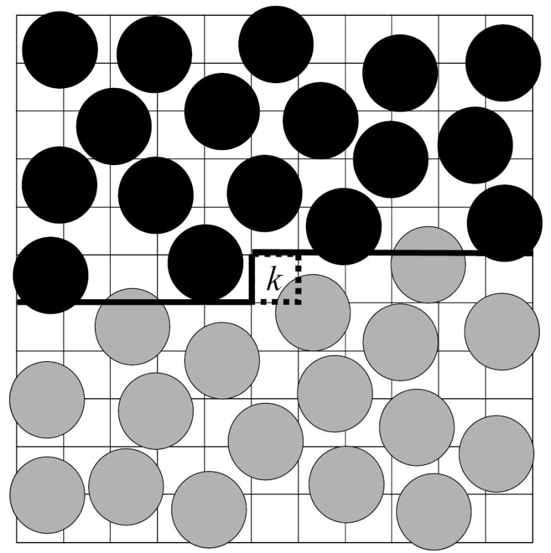
A two-dimensional (2D) illustration of the main simulation box at the kth step of the HSMC-EV reconstruction. The 2D “volume” is divided into cells, where k−1 of them have already been considered in previous steps (starting from the upper left corner). These k−1 cells comprise the “past volume” (the region above the heavy lines) which contains previously treated fixed atoms that are denoted by full black circles defined by the van der Waals radius. This region is excluded from the moveable future atoms (denoted by full grey circles) which are thus simulated in the “future volume” below the heavy lines, while in the presence of the fixed atoms. The future atoms can visit the target cell k (depicted by dotted lines) and their counts in this cell lead to the transition probability of an empty cell or the transition probability density of an occupied one. Note that for the case of an occupied target cell, counts are actually accumulated for visitations to a smaller region, Vcube (see text) located inside the target cell but not shown in the figure. For the case of HSMC(MD)-FV, the black atoms are again fixed, however, the volume is not partitioned into cells, and the (centers of the) grey atoms would be allowed to move above the heavy lines.
The transition probabilities are calculated (from the counts) in the following way. We denote by Mtot the total number of attempted moves in the MC simulation for any reconstruction step k. Mcell is the number of counts for which an atom was observed in the target cell k. The probability for the target cell to be occupied (unoccupied) by an atom is thus given by
| (22) |
For the case where the target cell k is vacant in configuration i, the transition probability is TPk=Punocc. For an occupied target cell, one has to calculate the probability density, ρocc, for an atom to be located at the precise location (inside cell k) at which it is found in configuration i. For this we define a much smaller volume (inside cell k), termed a “cube”, which is centered at x′, the exact atom position (target position). We count the visitations of atoms within this cube during the MC simulation and thus estimate the probability density as
| (23) |
where Mcube is the number of cube counts and Vcube is the cube volume. For occupied target cells TPk=ρocc. Note, however that the probability density is assumed to be uniform over the cube volume. To increase the quality of the results, we actually scale ρocc by an ensemble averaged weighting factor (see below), which serves to measure the probability density at the atom position more accurately.
The total product of TPk over all L3 cells – a product of N transition probability densities ρocc and L3-N transition probabilities for empty cells, gives rise to the estimate, ρHS (xN) for the Boltzmann probability density, ρ(xN),
| (24) |
Notice that the counting procedure (for the TPk) does not distinguish between labeled atoms, while in the integration leading to ZN all the labeled arrangements contribute, hence ρ(xN) [Eqs. (17–19)] is a labeled probability density, and N! is required in Eq. (24). These points also apply for the HSMC-FV and HSMD-FV methods below.
E.2 HSMC-FV and HSMD-FV
Most of the basic ideas underlying HSMC-FV and HSMD-FV are the same as for the case of HSMC-EV (or at least very analogous). As before, at step k we will again have Nk fixed atoms (and their images), and Nf = N − Nk future atoms which are allowed to move. An MC or MD trajectory (corresponding to HSMC-FV or HSMD-FV, respectively) is carried out for the future atoms in the presence of the Nk fixed (past) atoms, and the appropriate atom counts are accumulated. (See comments on TP calculations below.) However, during these simulations, there are no regions in the simulation box that the particles are excluded from. This proves to be a particularly desirable feature for the HSMD method. Specifically, in an HSMD-EV implementation, atoms would need to be reflected off of the excluded volume. While this can be fairly readily applied in MC (by simply rejecting moves), these reflections would prove to be somewhat more cumbersome for MD. For the FV case, rather, the only forces on the future atoms come from the Lennard-Jones interactions, and thus the future atoms will typically enter spaces between fixed atoms that would have otherwise been unavailable with EV. (The centers of the atoms can move above the heavy lines in Fig. 1.) Indeed they must sample these regions to arrive at the correct FV-TP.
As described for the case of “ideal HS”, the FV treatment simply requires N transition probabilities corresponding to probability densities of the form in Eq. (21). (Again, there are no TPs for empty cells.) Thus for HSMC(MD)-FV, one simulates, for each step k, the Nf future atoms in the presence of the Nk fixed atoms (and their images), with no explicit restrictions placed on the range of the future atoms. The probability (density) for a future atom to be located at the target position x′, is directly measured through raw counts, which is again done by centering a small counting cube at x′. The resulting transition probability density, ρx′,FV = TPk, is calculated as,
| (25) |
This is the same expression as for ρocc in Eq. (23), however the important difference is the different simulation conditions (FV vs. EV), therefore the TP densities are different. It should be noted that Mtot was defined above as the total number of attempted MC moves. For the case of HSMD, we define Mtot as the total number of MD time steps taken, and Mcube as the number of these time steps for which a future atom was found in the cube. Also, as for the case of HSMC-EV, we correct for the assumption of uniform probability density (within the cube) by scaling by an ensemble averaged weighting factor (see below). Finally, the HS estimate for overall probability density of the liquid configuration, ρHS (xN), is calculated as a product of the TPs according to Eq. (24), where here for FV, k runs from 1 to N.
The FV implementation is clearly simpler than EV, and it requires fewer HSMC(MD) simulations (N, rather than L3); furthermore, it is also exact in the limit of infinite sampling. However, some points should be made with regard to sampling TPs in practice. For some fixed atom geometries, it may be practically impossible to use standard MC and MD methods to correctly sample the probability distribution specified in Eq. (21). Open spaces that are blocked by fixed atoms can not be accessed by the moveable future atoms. Eq. (21) requires, in principle, that the future atoms be able to range over the entire volume, V. Therefore, if regions with nonnegligible Boltzmann weights are not sampled in the HSMC(MD)-FV simulations, then the calculated PiHS will be incorrect. The EV method is less prone to these dangers, as various pockets get treated (and excluded) before fixed atoms might potentially block them. For this reason, our FV implementation follows the geometrically organized order of treatment described at the end of Sec. II.D.2. The fixed atoms are grouped into consolidated regions (such as the black atoms in Fig. 1), and the very low Boltzmann weight for the future atoms in such regions (i.e., wholly among the black atoms), thus relaxes the need to sample this portion of the liquid volume in practice.
F. Implementation details and enhancements of the method
Several enhancements to the HSMC(MD) methods have been implemented. For the case of HSMC we apply MC preferential sampling,33–36 which imposes more frequent trial moves for atoms which are close to the target position x′ (or to the target cell for the case of EV). In our implementations the trial probability of each atom is proportional to 1/r2, where r is the atom’s distance measured from x′ (or the center of the target cell). The MC acceptance criterion is correspondingly altered so as to maintain detailed balance. To keep the trial probability from becoming arbitrarily large at small r, the weighting becomes flat for r2 less than ~3Å2. Additionally for the case of HSMC, it is beneficial to allow the number of MC steps at each reconstruction step (Mtot) to decrease (on average) as the number of future atoms decreases (i.e. with increasing k). This procedure maintains a roughly constant number of MC steps per future atom. In particular, we allow the maximum number of steps to depend linearly on the number of future molecules (until there are fewer than 20, in which case it is constant - see below).
Furthermore, for both HSMC and HSMD, the total run length for any particular step k is also based on its estimated sampling difficulty, which is determined from preliminary cube/cell counts accumulated during the equilibration period. In other words, longer run times are given to steps (k) that would be expected to have low transition probabilities. If, for example, very few cube counts are accumulated during the equilibration period, then the maximum number of steps is performed in the production run. Otherwise, for cases of higher preliminary counts, the run length is shorter (scaled down). There are many ways to carry out this weighting. We use several empirical settings (discrete categories) through which the number of steps is reduced from the maximum number (by up to a factor of about 5). For the case of EV, we further suggest treating occupied and unoccupied cells separately. As the unoccupied cells tend to be far easier to count reliably, significantly fewer steps should be allotted to them on average. Additional discussions of the above topics are available in Refs. 19 and 21.
Another important modification is the ensemble averaged weighting factor (mentioned above), which gives more accurate transition probability densities. This is computed during the HSMC or HSMD simulation in the following way. Every time an atom is found in the cube (defined above), we calculate the resulting (hypothetical) potential energy for this atom to be repositioned the exact location (inside the cube) at which an atom was exhibited in configuration being analyzed, that is, the target position, x′, at the center of the cube. This is done keeping all other atoms fixed. (In other words, all of the other Nf − 1 future atoms, and the Nk past atoms, remain fixed.) We denote this energy as E(x′; xN−1) and compare it to E(xN), the actual “undisplaced” potential energy of the system (as it was found in the HSMC or HSMD simulation), where it is recognized that the only difference between these two energies is due to the pairs involving the atom to be displaced. The ensemble average, 〈exp[− E(x′; xN−1) − E(xN)]/kBT〉cube, is computed over all cases (during the HSMC or HSMD simulation) where an atom is found (anywhere) in the cube. The transition probability density, ρx′,EV or ρx′,FV, [compare with Eqs. (23) and (25)] is then calculated as
| (26) |
Typical values for the ensemble average (in brackets) are on the order of 1. Nevertheless, these scaled corrections improve the overall results significantly. A detailed derivation of the weighting factor is given in the Appendix of Ref. 19.
Provided that the ensemble averaged weighting factor is used, implementations with different values for Vcube will always yield the correct free energy, F in the limit of infinite sampling. However, for finite length runs the quality of the free energy bound, FA, is affected by the size of Vcube. Generally, the ensemble averaged weighting factor (which is a function of cube size) will converge more readily as Vcube is made smaller, but a cube that is too small will lead to statistically unreliable cube counts. Thus, cube sizes at either extreme (too large or too small) will give rise to higher fluctuations and lower (poorer) values of FA.
The following points should be considered when choosing Vcube. The probability density is most sensitive to repulsive van der Waals overlaps; therefore, Vcube should be small on a scale of the molecular size. Still, a considerable range of Vcube values can give acceptable performance. For example, defining VvdW = (4/3)π(σ/2)3 as the molecular size of argon, we have found that values of Vcube/VvdW ranging from 5×10⁻⁵ to 1×10⁻² work reasonably well. Though we have not done a systematic optimization, the results reported in this work were generated using Vcube/VvdW values of about 2×10⁻³.
G. Simulation details
The argon system (also studied in Refs. 20 and 21) is comprised of 64 atoms at T=96.53K and reduced density, ρ*=Nσ3/V=0.846. In all cases the interactions were spherically truncated at a distance equal to half the box length, and the long-range energy (tail) corrections were added to the results.33 The box length for this system is 14.4 Å. The length and volume of the counting cube are 0.3429 Å and 0.04032 Å3, respectively. The cell length and volume (for the EV case) are 2.40 Å and 13.8 Å3, respectively.
The sample configurations (which are analyzed in the HSMC and HSMD procedures) were generated using the usual Metropolis MC simulation method 6 in the (NVT) ensemble under periodic boundary conditions. Thus, at each MC step an atom is selected at random and a random translational trial move is generated within a small Cartesian cube around the atom position. Step sizes were chosen to give ~40–50% acceptance. Configurations were recorded at long enough intervals to give an uncorrelated sample.
The MC simulations of the future molecules during the HS reconstruction process (HSMC-EV and HSMC-FV) are very similar to the standard MC simulations. The exceptions (which were discussed above) are: the system is only partially mobile (Nk atoms are fixed), the atoms are selected preferentially for trial moves based on their proximity to the target position (or cell), and for the EV case, the moveable future atoms are excluded from the previously treated regions. Additionally, the number of MC steps (Mtot) for HS reconstruction step k was not constant but varied with the number of future molecules and other criteria outlined in Sec. II.F. The results (Table I) are therefore given as a function of the average number of MC steps per atom, per reconstructed configuration. This is denoted by MαMC, and thus defines the level of approximation, α; the longer the HSMC simulations (larger MαMC), the better the approximation. A single HSMC (or HSMD) reconstruction is performed on each sample configuration, and the overall results are determined by averaging over a total sample size of n configurations. (e.g., an arithmetic average of FiHS is taken for FA, etc.). The results for HSMC-EV are taken from Ref. 21.
Table I.
HSMD and HSMC free energy results for liquid argon.a
| MαMC(MD) | -FA | σA | -FB | -FGB | -FM | -FGM | -FD | R | n |
|---|---|---|---|---|---|---|---|---|---|
| HSMC-EV - Explicit Treatment of Excluded Volume | |||||||||
| 24 ×105 | 4.132 (1) | 0.0330 (5) | 4.064 (4) | 4.046 (3) | 4.098 (4) | 4.089 (2) | 4.096 (3) | 0.11 | 581 |
| 48 ×105 | 4.117 (1) | 0.0224 (5) | 4.079 (4) | 4.077 (2) | 4.098 (4) | 4.097 (1) | 4.098 (3) | 0.19 | 495 |
| 96 ×105 | 4.1085 (8) | 0.0167 (5) | 4.087 (3) | 4.086 (2) | 4.098 (3) | 4.097 (1) | 4.097 (2) | 0.38 | 459 |
| 240 ×105 | 4.1046 (5) | 0.0105 (5) | 4.096 (2) | 4.096 (1) | 4.100 (2) | 4.1002 (7) | 4.100 (1) | 0.53 | 371 |
| 480 ×105 | 4.1025 (5) | 0.0078 (3) | 4.097 (1) | 4.0976 (6) | 4.100 (1) | 4.1001 (5) | 4.1000 (8) | 0.60 | 244 |
| 960 ×105 | 4.1019 (4) | 0.0053 (5) | 4.099 (1) | 4.0997 (6) | 4.100 (1) | 4.1008 (5) | 4.1007 (8) | 0.76 | 174 |
| -FTI | 4.100 (1) | ||||||||
| HSMC-FV - Free Volume Treatment | |||||||||
| 18 ×105 | 4.119 (1) | 0.0231 (9) | 4.084 (1) | 4.076 (4) | 4.1014 (8) | 4.097 (2) | 4.0994 (9) | 0.27 | 531 |
| 36 ×105 | 4.1109 (8) | 0.0177 (5) | 4.090 (1) | 4.086 (2) | 4.1006 (7) | 4.098 (1) | 4.0997 (7) | 0.37 | 484 |
| 72 ×105 | 4.1062 (6) | 0.0135 (6) | 4.0911 (7) | 4.092 (1) | 4.0987 (5) | 4.0990 (9) | 4.0987 (6) | 0.40 | 575 |
| 180 ×105 | 4.1016 (5) | 0.0097 (3) | 4.0930 (7) | 4.0941 (7) | 4.0973 (4) | 4.0978 (5) | 4.0975 (5) | 0.52 | 412 |
| 360 ×105 | 4.1003 (4) | 0.0083 (3) | 4.0935 (8) | 4.0949 (6) | 4.0969 (4) | 4.0976 (5) | 4.0971 (6) | 0.61 | 414 |
| 720 ×105 | 4.0998 (4) | 0.0071 (4) | 4.0946 (8) | 4.0958 (6) | 4.0972 (5) | 4.0978 (5) | 4.0974 (6) | 0.59 | 251 |
| -FTI | 4.100 (1) | ||||||||
| HSMD-FV - Free Volume Treatment | |||||||||
| 1 ×10⁷ | 4.146 (2) | 0.036 (2) | 4.082 (3) | 4.04 (1) | 4.114 (2) | 4.094 (5) | 4.106 (3) | 0.15 | 475 |
| 2 ×10⁷ | 4.122 (1) | 0.0247 (5) | 4.081 (3) | 4.073 (2) | 4.1016 (9) | 4.098 (2) | 4.100 (1) | 0.20 | 464 |
| 4 ×10⁷ | 4.1095 (9) | 0.0189 (4) | 4.086 (2) | 4.081 (2) | 4.0979 (9) | 4.095 (1) | 4.0968 (9) | 0.37 | 471 |
| 10 ×107 | 4.1041 (7) | 0.0144 (4) | 4.089 (1) | 4.088 (1) | 4.0963 (7) | 4.0958 (8) | 4.0960 (9) | 0.41 | 480 |
| 20 ×107 | 4.1017 (7) | 0.0112 (5) | 4.0922 (9) | 4.092 (1) | 4.0969 (6) | 4.0967 (9) | 4.0968 (7) | 0.54 | 241 |
| 20 ×107* | 4.0996 (6) | 0.0097 (4) | 4.0921 (7) | 4.0921 (9) | 4.0958 (5) | 4.0959 (7) | 4.0958 (6) | 0.60 | 242 |
| −FTI | 4.100 (1) | ||||||||
N = 64 is the number of atoms, T = 96.53 K is the temperature, ρ* = Nσ3/V = 0.846, the reduced density, where V is the volume and σ is the standard Lennard Jones distance parameter. Free energy values are given as Ac/εN where Ac is the configurational free energy [Eq. (20)] and ε is the standard Lennard-Jones energy parameter. FTI was obtained by thermodynamic integration. FA [Eq. (7)] is a lower bound of the free energy and σA [Eq. (8)] is its fluctuation. FB [Eq. (10)] is an upper bound and FGB [Eq. (12)] is its corresponding Gaussian approximation. FM [Eq. (13)] and FGM [Eq. (14)] are the averages of FA with FB and FGB, respectively. FD [Eq. (15)] is the direct estimate for the free energy. R [Eq. (11)] is the acceptance rate for the reversed-Schmidt procedure. MαMC is the average number of MC steps per atom, per reconstructed configuration. MαMD is the average number of MD steps per configuration, where the “*” in the last row corresponds to a 10 fs time step. (The other results are for a 5fs time step.) n is the number of configurations analyzed (the sample size), where a single HSMC(MD) reconstruction was performed on each configuration. The statistical error appears in parenthesis; for example, 4.098(3) = 4.098±0.003. It is noted that FA and σA are reported here as per atom quantities, however, Eq. (12) as written for FGB requires these quantities to be for the system as a whole. (See Ref. 21.) Thus the values given here must be multiplied by N before using Eqs. (12) and (14) for FGB and FGM, respectively.
The MD simulations of the future molecules (HSMD-FV) are also very similar to standard MD liquid simulations, with again the exception that Nk of the atoms are held fixed. The trajectories are integrated with the velocity form of the Verlet algorithm.37 Most of the simulations were performed with a time step of 5 fs, however a time step of 10fs was also used. The temperature was maintained with an Andersen bath,38 where all velocities (of the moveable future atoms) were reassigned from a Maxwell-Boltzmann distribution at time intervals of 2.5 ps. As for HSMC, the run lengths at each HS reconstruction step k varied depending on the estimated sampling difficulty, and therefore we report HSMD results as a function of the average number of MD steps per reconstructed configuration, denoted MαMD. We note finally that atom counts for the case of HSMD were actually accumulated in a sphere centered at x′, rather than a cube. The volume of this sphere is the same as the volume of the cube (above) used in HSMC. As observed from shorter test runs, the difference in these choices is small.
Several studies of the free energy of argon 29,31,32,39–43 have been published, most of them for systems that differ in size (as well as other modeling details) from the present one. Therefore, for an objective evaluation of our results, we also calculated the free energies for our particular system of argon using thermodynamic integration (TI). The Lennard-Jones interactions were scaled using the shifted scaling potential of Zacharias et al.44 A more detailed description of our TI calculations is available in Ref. 17.
Free energy results are presented in Table I. All values correspond to the configurational free energy, Ac [Eq. (20], per atom, and in energy units of ε (i.e., Ac/εN). Shown here are the free energy estimates FA, FB, FGB, FM, FGM, and FD, and the fluctuation in FA, σA. These free energy estimates are given as a function of either MαMC or MαMD (for HSMC or HSMD, respectively). As described above, MαMC (or MαMD) defines the level of approximation (α), where the largest values correspond to the best approximations. The free energy determined by TI for this particular argon system is −4.100 (+/− 0.001). We take this as the correct value.
III. RESULTS AND DISCUSSION
A. Results for HSMC-EV
We will first briefly summarize the results for HSMC-EV which were presented previously (Ref. 21). This will provide an acquaintance with the behavior of the various free energy functionals and aid in our comparisons with the new results for the FV treatment. The lower bound, FA [Eq. (7)], clearly shows the expected trends where the values steadily increase (improve), and approach convergence, as MαMC is increased. FA for the largest MαMC deviates from the TI value by less than 0.05%. (The statistical error in the TI result is ~0.02%.) The worst approximation, based on 40 times smaller MαMC still leads to a free energy estimate that is only ~0.8% lower than the TI value. The fluctuation, σA, in FA [Eq. (8)] also shows the expected trends, as its values consistently decrease as the approximation improves. (i.e., σA tends toward zero as FA approaches the correct value.) This behavior in the fluctuations reflects the reliability of the various free energy estimates. σA is particularly important for FGB and FGM (discussed below), as their calculation is derived directly from its value.
We noted in Ref. 21 the excellent quality (statistical reliability) of the other free energy estimates. The free energy upper bound FB [Eqs. (9, and 10)] steadily decreases (improves) as MαMC is increased. The FB value for the best approximation agrees with the TI result within the statistical uncertainty. The worst approximation deviates by only 0.9%. The Gaussian upper bound estimate FGB is in very good agreement with FB and thus shows similar converging behavior as the approximation improves. Highly accurate results are obtained for FM and FGM [Eqs. (13) and (14)], which are the averages of the lower (FA) and upper bounds (FB or FGB). Similar accuracy is also observed for the direct free energy estimate FD [Eq. (15)]. The best three approximations (MαMC) lead to values of FM, FGM and FD that match the TI value within the statistical uncertainty. In all cases FM, FGM and FD provide a better value for the free energy than the corresponding bound estimates FA, FB, or FGB at the same MαMC. As mentioned in Sec. II.B, the statistical reliability of FB and FD can be limited by insufficient overlap of the distributions, PiB and PiHS. The values of the acceptance rate, R, [Eq. (11)] for the “reversed-Schmidt procedure”12,15 (given in the table) provide a convenient gauge of this overlap, the larger is R, the better the overlap. The smallest R (~0.1) for the worst approximation is considered to be adequate (for the sample size, n), and it is seen that R steadily increases as the approximation improves.
B. Results for HSMC-FV
Before discussing the results for the new FV treatment (HSMC(MD)-FV). It should be noted that we have found it beneficial to eliminate a small fraction of the configurations from the sample. That is, we consider 95% of the reconstructed configurations, where those that resulted in the most deviant FiHS values (from the average, in either direction) were eliminated. This was not done in the EV results, and thus we will more fully discuss below why this is done for the case of FV. It is stressed however, that cutting this number of configurations from the sample has minimal effects on FA (which is the most reliable and important estimate). In no case was the change in the calculated FA more than 0.05%. This is comparable, for example, to the statistical error in the TI calculation (0.02%).
Starting with the results for HSMC-FV (Table I), we again see the expected general behavior for the various free energy functionals. The lower bound, FA, consistently increases and its fluctuation, σA, decreases as the approximation improves. The FA values for the two largest MαMC agree (within the uncertainty) with the TI result (−4.100). Similarly, the upper bounds, FB and FGB, consistently decrease as MαMC increases. Their values for the best approximation deviate from the correct value by only ~ 0.1%, however, this deviation is larger than for the best approximations in the case of HSMC-EV. For the three lowest approximations, the averages of the lower and upper bounds, FM or FGM, clearly provide a better value for the free energy than the corresponding bound estimates FA, FB, or FGB, where the maximum deviation from the correct value is less than 0.1%. FD is similarly superior to the bounds in these cases. In the case of the two highest MαMC, on the other hand, FM, FGM and FD deviate by more than does FA. The maximum deviation is still less than 0.08% however. (A discussion of the difference in accuracy of EV and FV at the highest approximations will be deferred until after the HSMD results have been presented.)
We noted that a potential advantage of HSMC-FV is that it requires fewer simulations because TPs for empty cells are not calculated. It is therefore interesting to compare the efficiency of HSMC for the cases of EV and FV. A good way to do this is to compare the tightness of the free energy bounds as a function of computational time. In Fig. 2 we give the lower and upper bounds for the first four approximations of HSMC-EV and HSMC-FV. (The lower bound is FA, while the upper bound is the average of FB and FGB. Computational times are given on the x-axis in CPU hours per configuration on an AMD 2400.) The difference in the tightness of the bounds is quite striking, with the values for FV appearing well inside those for EV. As an example, the bounds for the second approximation of HSMC-FV (requiring 0.5 hrs./config.) are very comparable (similar separation and average value) to the bounds for the third approximation of HSMC-EV (requiring 1.44 hrs./config.). This implies an increase in efficiency for HSMC-FV by a factor of two or three over the previous EV treatment.
Fig. 2.
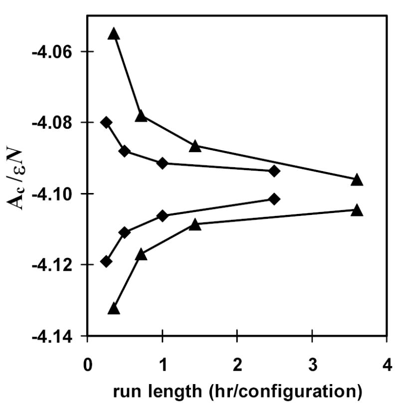
Free energy bounds as a function of computational time for liquid argon: comparison of HSMC-FV and HSMC-EV. The HSMC run length on the horizontal axis is given in CPU hours of computational time (AMD 2400) per reconstructed configuration. Shown for both methods are the free energy lower bound FA, and the upper bound, which is the average of FB and FGB. The diamonds represent the results for HSMC-FV, while the triangles correspond to HSMC-EV. Free energies are given as Ac/εN, where Ac is the configurational free energy defined in Eq. (20), ε is the standard Lennard-Jones energy parameter, and N is the number of atoms.
C. Results for HSMD-FV
We now summarize the results for the HSMD-FV method. It is noted that the approximations go as MαMD in the first five rows of HSMD results in Table I, however, MαMD = 20 ×107 appears a second time in the sixth row. This is the highest approximation which was run using a 10 fs time step (rather than 5 fs). The HSMD-FV results also show well the expected general behavior for the free energy functionals. FA consistently increases and σA decreases as the approximation improves. The FA result for the best approximation agrees with the TI value (−4.100) within the statistical uncertainty, while the worst approximation gives an FA value that is only ~1% lower. The upper bounds, FB and FGB, consistently decrease as MαMD increases, with values for the best approximation deviating from the correct value by only ~0.2%, but more so, than for HSMC-EV. Similar to HSMC-FV, FM, FGM and FD for the three lowest approximations, are much closer to the correct free energy than the corresponding bound estimates FA, FB, or FGB, while they deviate more than FA in the case of the two highest approximations. Again, the results for FM, FGM and FD for the best approximations are still very good, deviating by only ~0.1% or less.
It is worth noting that we find no dependence of our results on the choice of time step (5 or 10 fs). As mentioned, the best approximation was calculated using the larger 10 fs time step. Furthermore, we have obtained additional results (not given) using a 10 fs time step for the case of MαMD = 5 ×10⁷ steps (sample size, n = 160 configurations). The results for all of the free energy functionals and the fluctuations are the same as the tabulated results for MαMD = 10 ×107 (using a 5 fs time step) within their statistical errors.
We now compare the efficiency of HSMD-FV to that of the previous HSMC-EV method. Again we assess the tightness of the lower and upper free energy bounds for the four lowest approximations as a function of computational time. These values are plotted in Fig. 3. (The HSMD times have been scaled for a 10 fs time step. The upper bound is again the average of FB and FGB.) The trend lines trace each other fairly well. Therefore the efficiency of the two methods (HSMD-FV and HSMD-EV) is about the same. This does imply however, that this HSMD-FV implementation is not as efficient as HSMC-FV. This is most likely attributable to the MC preferential sampling performed in the latter. As described above, atoms that are close to the target position are chosen for MC moves more frequently. This is a highly beneficial modification given the observables we wish to track in the simulation (i.e. counts at the target position). Indeed the implementation of preferential sampling gave rise to substantial improvements during the initial development of HSMC.
Fig. 3.
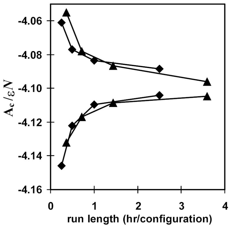
Free energy bounds as a function of computational time for liquid argon: comparison of HSMD-FV and HSMC-EV. The HSMC(MD) run length on the horizontal axis is given in CPU hours of computational time (AMD 2400) per reconstructed configuration. Shown for both methods are the free energy lower bound FA, and the upper bound, which is the average of FB and FGB. The diamonds represent the results for HSMD-FV, while the triangles correspond to HSMC-EV. Free energies are given as Ac/εN, where Ac is the configurational free energy defined in Eq. (20), ε is the standard Lennard-Jones energy parameter, and N is the number of atoms.
D. Discussion of the FV treatment
One of the similarities of HSMC-FV and HSMD-FV is the fact that the lower bound values (FA) for the highest approximations actually reach the TI value, while the functionals, FM, FGM and FD, (which at times should be considered more accurate) are greater than this value (lying outside the statistical uncertainty). This is not exhibited in the HSMC-EV results. Here, the FM, FGM and FD values become highly accurate for the three best approximations. (Note also that the fluctuations and R values for FV do not become quite as low and high respectively as they do for EV at the highest approximations.) For the FV treatment, there thus appears to be a slight skewing of the results, pushing the free energies to slightly higher values. These effects, for example, start to become visibly apparent by the fourth approximation in Figs. 2 and 3. It is further noted that beyond the fourth approximation, the bounds actually become tighter for EV. In general, the FV treatment does not provide the high accuracy ultimately provided by EV.
Though the skewing of the FV results is small (0.1% or less), it is important to analyze this shortcoming in terms of the assumptions of the method. In particular, we pointed out in Sec. II.D.2 that the TPs are based on a configuration space (for the future atoms) that covers the entire liquid volume, V. In practice, with MC or MD sampling, the future atoms do not visit the entire volume due to repulsive interactions from the fixed atoms. Therefore we rely on the assumption that any region that can not be accessed with the usual sampling/simulation methods, does not need to be accessed, due to a low Boltzmann weight for that region. Problems will arise however if fixed atoms block future atoms from accessing regions with non-negligible weight. This is why we reconstruct the configuration in a way that groups the fixed atoms together. In other words, we try to make a reasonably contiguous region of low Boltzmann weight that does not need to be sampled by the future atoms. Inevitably, there will be some cases where pockets are formed among the fixed atoms that can not be accessed. (The EV treatment can treat and exclude these pocket regions before they get blocked off.) Thus for FV, these occasional situations will affect the counts for the TP, and therefore the calculated free energy.
One can make some rough arguments for the direction that these sampling problems will push the results. We note that at the beginning of every HSMC(MD) simulation we start from the exact coordinates of configuration i. (This is for both fixed and future atoms.) It is important to point out that the future atoms must be well equilibrated before the counting begins, because this would otherwise skew the results by consistently giving “bonus counts” at the beginning of the simulation, due to the fact that a future atom always starts at the target position, x′. Now, if we have at some reconstruction step k, a situation where there is a non-negligible region that can not be accessed by the future atoms, the actual sampling is thus restricted to a smaller configuration space. Furthermore, because this restricted space contains geometries with an atom at/near the target position, it will likely favor these geometries. Said another way: If the simulation always starts from a region of configuration space that is at least partially defined by an atom at/near x′ and a matching geometry of future atoms surrounding it, then sampling bottlenecks serving to keep the system in that region should typically lead to erroneously high counts at the target position. This implies that the TP would be too high, making the overall probability estimate, PiHS, too high, and thus FiHS [Eq. (5)], and the resulting free energy functionals, will be too high.
Because these sampling problems are related to particular fixed atom geometries (that cause the sampling barriers), it is very reasonable to guess that certain configurations are more prone to give skewed free energy estimates (FiHS) when analyzed with an FV treatment. Indeed, this is the case. We have found for example, that very often the most drastically deviant (high) FiHS values come from the same handful of configurations. This is regardless of the method, HSMD-FV or HSMC-FV, or the particular level of approximation. (The various HSMC and HSMD runs are always performed using the same file of sample configurations.) Adjusting the order of the build up procedure would likely improve the results for some of these structures, however for other “well behaved” structures, it could make the results worse.
We discussed above the effects of sampling barriers on the value of FiHS and how it serves to lower the free energy estimates. Again, the effect is relatively small, only being a problem for certain configurations (or individual reconstruction steps k). However, a handful of deviant FiHS values can have a strong effect on certain free energy functionals. Good examples of this are FD and FB [Eqs. (10) and (15)]. Their calculation depends on an exponential average of FiHS, that can easily become dominated by a single configuration with an unusually high FiHS. FGB is also effected, because the fluctuations are sensitive to very deviant values. This sensitivity is why we only consider 95% of the FiHS values in calculating the FV results. It should be noted however, that the straightforward arithmetic average of FiHS (FA) is the least affected by deviant FiHS values. (We mentioned above that FA never changed by more than 0.05% when deviants were eliminated.) This is an important point because FA (which converges more rapidly than any of the other free energy functionals) will often be the primary estimate in many practical investigations where only a small sample (e.g. n ≈ 5 – 20) is analyzed. (Note that these situations can still be augmented by a (rough) estimate for σA, and therefore an estimate for FGB, which can be used as a guide in bracketing the correct value.)
It follows that the utility of the FV treatment as compared to EV depends largely on the desired accuracy for any particular investigation. If one requires highly accurate results, EV should be used. However, one might more typically desire an accuracy around 0.5% or less. Here, FV is clearly the better choice. The implementation is much simpler, and for the case of HSMC-FV, it is more computationally efficient. Furthermore, this level of accuracy is very attainable with the lower bound functional FA alone, which (as discussed above) is only mildly affected by the FV treatment.
IV. SUMMARY AND CONCLUSIONS
In this paper we have introduced the HSMD method for liquids. In order to do this we have modified our previous HS treatment which explicitly calculated the transition probabilities for excluded (empty) volumes (EV) and thus introduced a new free volume (FV) treatment. The FV approach was tested first as a variant of HSMC (HSMC-FV) and then successfully applied for molecular dynamics as HSMD-FV. Both the HSMD-FV and HSMC-FV results agree well (within 0.1% or better) with our TI results, as well as our previous HSMC-EV results. The efficiency of HSMD-FV is equivalent to that of HSMC-EV, while the efficiency of HSMC-FV has improved on HSMC-EV by more than a factor of two. We have discussed some of the differences between the EV and FV treatments, including a slight skewing of the results that occurs for FV due to sampling difficulties posed by fixed atoms in the simulations. This deviation is not expected to be troublesome in most practical applications.
Though the HSMC(MD) methods continue to be improved, at this time they are still less efficient than TI. The TI run for this argon system required 1.2 hours on an AMD 2400. A single reconstruction using HSMC-FV with MαMC = 72 ×105 requires 1 hour, and will yield essentially the same free energy value, but with a statistical uncertainty that is 10 times larger. (Still this is only +/−0.3%). The precision can be improved by reconstructing several more configurations and averaging FiHS. Furthermore, unlike other methods, the fluctuation (σA) can be estimated for this very small sample giving rise to a rough upper bound estimate (FGB) that can be used to bracket the correct value, thus the giving the methodology its own “self-checking” mechanism. While with TI, an ideal gas is integrated by gradually changing the potential energy parameters to their final values, the HSMC(MD) methods, on the other hand, are quite different. The absolute free energy is obtained, in principle, by reconstructing a single configuration, i.e., placing its molecules gradually into their positions using transition probabilities. Therefore, the HSMC(MD) methods constitute new research tools independent of TI and related methods, which enables one to calculate F by analyzing a given MC or MD sample. HSMC(MD) is general and can be applied to a variety of systems. However, clearly the implementation of HSMC(MD) is somewhat more complex than TI.
This methodology is expected to be useful in particular for protein systems. Thus, peptides and segments of proteins such as surface loops are typically flexible populating several microstates in thermodynamic equilibrium (a microstate is defined by the local conformational fluctuations around a structure such as the α-helical structure of a peptide). Calculating the free energies (hence the relative populations) of such microstates is important in structural biology, however, it becomes an extremely difficult task to achieve with the conventional methods. HSMC(MD) has been applied successfully to peptides in vacuum and a recent study has shown that differences ΔFm,n = Fm −Fn between microstates can be obtained with high accuracy already for limited computational investments (small MαMD values) due to the fact that systematic errors in Fm and Fn are similar and they are cancelled in Δ Fm,n. We intend to apply HSMD to a loop capped with water molecules where the system is simulated by MD. In this case the loop is reconstructed initially in the presence of moving waters, and the configuration of the water molecules is reconstructed next in the presence of a “frozen” loop structure. The latter reconstruction can be carried out by HSMC(MD)-FV described here. Because our main interest is in free energy differences we expect the required computer time for calculating Δ Fm,n for water to be significantly smaller than that that would be required for a reasonable accuracy of the absolute values, Fm and Fn themselves.
Acknowledgments
This work was supported by NIH grants R01 GM61916 and R01 GM66090
References
- 1.Beveridge DL, DiCapua FM. Annu Rev Biophys Biophys Chem. 1989;18:431. doi: 10.1146/annurev.bb.18.060189.002243. [DOI] [PubMed] [Google Scholar]
- 2.Kollman PA. Chem Rev. 1993;93:2395. [Google Scholar]
- 3.Jorgensen WL. Acc Chem Res. 1989;22:184. [Google Scholar]
- 4.Straatsma TP, McCammon JA. Annu Rev Phys Chem. 1992;43:407. [Google Scholar]
- 5.Meirovitch H. In: Reviews in Computational Chemistry. Lipkowitz Kenny B, Boyd Donald B., editors. Vol. 12. Wiley; New York: 1998. p. 1. [Google Scholar]
- 6.Metropolis N, Rosenbluth AW, Rosenbluth MN, Teller AH, Teller E. J Chem Phys. 1953;21:1087. [Google Scholar]
- 7.Alder BJ, Wainwright TE. J Chem Phys. 1959;31:459. [Google Scholar]
- 8.McCammon JA, Gelin BR, Karplus M. Nature. 1977;267:585. doi: 10.1038/267585a0. [DOI] [PubMed] [Google Scholar]
- 9.Meirovitch H. Chem Phys Lett. 1977;45:389. doi: 10.1016/j.cplett.2005.06.002. [DOI] [PMC free article] [PubMed] [Google Scholar]
- 10.Meirovitch H. Phys Rev B. 1984;30:2866. [Google Scholar]
- 11.Meirovitch H, Vásquez M, Scheraga HA. Biopolymers. 1987;26:651. doi: 10.1002/bip.360260508. [DOI] [PubMed] [Google Scholar]
- 12.Meirovitch H, Koerber SC, Rivier J, Hagler AT. Biopolymers. 1994;34:815. doi: 10.1002/bip.360340703. [DOI] [PubMed] [Google Scholar]
- 13.Chorin AJ. Phys Fluids. 1996;8:2656. [Google Scholar]
- 14.Meirovitch H. J Phys A. 1983;16:839. [Google Scholar]
- 15.Meirovitch H. Phys Rev A. 1985;32:3709. doi: 10.1103/physreva.32.3709. [DOI] [PubMed] [Google Scholar]
- 16.Meirovitch H. J Chem Phys. 1999;111:7215. [Google Scholar]
- 17.Szarecka A, White RP, Meirovitch H. J Chem Phys. 2003;119:12084. [Google Scholar]
- 18.Meirovitch H. J Chem Phys. 2001;114:3859. [Google Scholar]
- 19.White RP, Meirovitch H. J Chem Phys. 2003;119:12096. [Google Scholar]
- 20.White RP, Meirovitch H. Proc Natl Acad Sci USA. 2004;101:9235. doi: 10.1073/pnas.0308197101. [DOI] [PMC free article] [PubMed] [Google Scholar]
- 21.White RP, Meirovitch H. J Chem Phys. 2004;121:10889. doi: 10.1063/1.1814355. [DOI] [PubMed] [Google Scholar]
- 22.Cheluvaraja S, Meirovitch H. Proc Natl Acad Sci USA. 2004;101:9241. doi: 10.1073/pnas.0308201101. [DOI] [PMC free article] [PubMed] [Google Scholar]
- 23.Cheluvaraja S, Meirovitch H. J Chem Phys. 2004;122:054903-1. [Google Scholar]
- 24.Cheluvaraja S, Meirovitch H. J Phys Chem B. 2004;109:21963. doi: 10.1021/jp052969l. [DOI] [PMC free article] [PubMed] [Google Scholar]
- 25.White RP, Jason Funt, Meirovitch H. Chem Phys Lett. 2005;410:430. doi: 10.1016/j.cplett.2005.06.002. [DOI] [PMC free article] [PubMed] [Google Scholar]
- 26.White RP, Meirovitch H. J Chem Phys. 2005;123:214908-1. doi: 10.1063/1.2132285. [DOI] [PMC free article] [PubMed] [Google Scholar]
- 27.Meirovitch H, Alexandrowicz Z. J Stat Phys. 1976;15:123. [Google Scholar]
- 28.Gibbs W. Elementary Principles in Statistical Mechanics. Chapter XI. Yale University Press; 1902. [Google Scholar]
- 29.Li Z, Scheraga HA. J Phys Chem. 1988;92:2633. [Google Scholar]
- 30.Coldwell RL. Phys Rev A. 1973;7:270. [Google Scholar]
- 31.Gosling EM, Singer K. Pure Appl Chem. 1970;22:303. [Google Scholar]
- 32.Henchman RH. J Chem Phys. 2003;119:400. [Google Scholar]
- 33.Allen MP, Tildesley DJ. Computer simulation of liquids. Clarenden Press, Oxford; 1987. [Google Scholar]
- 34.Owicki JC. Computer modeling of matter. In: Lykos P, editor. ACS Symposium Series. Vol. 86. American Chemical Society; Washington: 1978. p. 159. [Google Scholar]
- 35.Jorgensen WL. J Phys Chem. 1983;87:5304. [Google Scholar]
- 36.Owicki JC, Scheraga HA. Chem Phys Lett. 1977;47:600. [Google Scholar]
- 37.Swope WC, Andersen HC, Berens PH, Wilson KR. J Chem Phys. 1982;76:637. [Google Scholar]
- 38.Andersen HC. J Chem Phys. 1980;72:2384. [Google Scholar]
- 39.Torrie GM, Valleau JP. Chem Phys Lett. 1974;28:578. [Google Scholar]
- 40.Torrie GM, Valleau JP. J Comp Phys. 1977;23:187. [Google Scholar]
- 41.Levesque D, Verlet L. Phys Rev. 1969;182:307. [Google Scholar]
- 42.Mezei M. Mol Simul. 1989;2:201. [Google Scholar]
- 43.Johnson JK, Zollweg JA, Gubbins KE. Mol Phys. 1993;78:591. [Google Scholar]
- 44.Zacharias M, Straatsma TP, McCammon JA. JChem Phys. 1994;100:9025. [Google Scholar]