Noise simulation in cone beam CT imaging with parallel computing

Abstract

We developed a computer noise simulation model for cone beam computed tomography imaging using a general purpose PC cluster. This model uses a mono-energetic x-ray approximation and allows us to investigate three primary performance components, specifically quantum noise, detector blurring and additive system noise. A parallel random number generator based on the Weyl sequence was implemented in the noise simulation and a visualization technique was accordingly developed to validate the quality of the parallel random number generator. In our computer simulation model, three-dimensional (3D) phantoms were mathematically modelled and used to create 450 analytical projections, which were then sampled into digital image data. Quantum noise was simulated and added to the analytical projection image data, which were then filtered to incorporate flat panel detector blurring. Additive system noise was generated and added to form the final projection images. The Feldkamp algorithm was implemented and used to reconstruct the 3D images of the phantoms. A 24 dual-Xeon PC cluster was used to compute the projections and reconstructed images in parallel with each CPU processing 10 projection views for a total of 450 views. Based on this computer simulation system, simulated cone beam CT images were generated for various phantoms and technique settings. Noise power spectra for the flat panel x-ray detector and reconstructed images were then computed to characterize the noise properties. As an example among the potential applications of our noise simulation model, we showed that images of low contrast objects can be produced and used for image quality evaluation.

1. Introduction

Cone beam computed tomography (CBCT) is a promising imaging modality and has been a research highlight in recent years, mainly because of the recent technological advent of x-ray flat panel detectors (Chen and Ning 2004, Hampton et al 2003, Mueller and Yagel 2000, Ning et al 2004). Two major types of CBCT reconstruction algorithm, Feldkamp (Feldkamp et al 1984) (based on weighted filtered backprojection) and ART (Hampton et al 2003, Mueller and Yagel 2000, Smith 1990) (based on algebraic iterations), and other variant methods, have been studied and improved in terms of accuracy and efficiency for years.

Many factors can affect the cone beam CT imaging performance such as the x-ray spectrum, photon scatter, focal spot blurring, scanning geometry, number of projections, scanner misalignment, detector blurring, detector pixel size, voxel size, reconstruction algorithms, quantum noise and electronics noise. Especially, several sources of errors and artefacts are associated with the presence of various noises that could affect the cone beam CT image quality. It is therefore necessary to assess their significance and consequence on the reconstructed images to reduce their impacts by either optimizing the scanner design or developing image correction-related algorithms.

The fluctuation in x-ray detection is an intrinsic property to the x-ray imaging and cannot be prevented with current technology (Chesler et al 1977, Riederer et al 1978). Noise in the reconstructed images is caused mainly by the photon statistics, and in this paper we refer to this type of photon fluctuation as quantum noise. The spatial resolution in the reconstructed images could be degraded by the flat panel detector blurring and is often characterized by the point spread function (PSF) or the line spread function (LSF). Additive system noise (Granfors and Aufrichtig 2000, Maolinbay et al 2000) that may originate from the scintillator structures or detector electronics was modelled in this study as well.

The scope of this paper is to present and discuss the techniques of using a parallel computing technique to simulate various types of noise in CBCT images. The noise power spectra (NPS) were computed to quantify the noise properties (Faulkner and Moores 1984, Hahn et al 1988, Kijewski et al 1991). To demonstrate the application, our noise simulation method was applied to the comparison of the two different types of filter (Ramp and Shepp–Logan) used in the Feldkamp algorithm. It was also used to generate images of analytically modelled phantoms at various noise level settings for the evaluation of low contrast performance. This paper was organized as follows. In section 2 we present the methodology including the development of a parallel random number generator based on the Weyl sequence and the master–slave programming model used in the paper. The results and their associated discussions are presented in section 3. A short summary of our study and suggested future research work are covered in section 4.

2. Theory and methods

In this section, we present the theory and background of the methods used in our noise simulation model. How we modelled the quantum noise, detector blurring and additive system noise is described in detail. A visualization technique based on the Feldkamp algorithm was developed to evaluate the quality of a parallel random number generator used in the noise simulation.

2.1. Noise and random number generator

Quantum noise production is a stochastic process by nature (Cheng et al 2004, Chesler et al 1977, Riederer et al 1978). People in the scientific community have been using numerical random number generators (RNG) for stochastic simulation such as Monte Carlo calculations for decades, and tremendous high-quality research work has been produced (Entacher et al 1999, Koniges and Leith 1989, Saarinen et al 1991, Srinivasan et al 2003). Conventional RNGs have been developed for the single central processing unit (CPU) computation. Now it is possible to use hundreds or even thousands of computing processors, either 32-bit or 64-bit, for intensive numerical applications. The computing capability for a trillion floating point operations per second (FLOPS) has also been available for the past few years. However, the research for implementing high-quality parallel random number generators (PRNG) for parallel programming is still in its early development stage (Ackermann et al 2001, Marchenko and Mikhailov 2002, Quinn 2004). Especially, there are only limited empirical statistical tests to quantify and test those PRNGs (Liang and Whitlock 2001, Srinivasan et al 2003). In this study, we applied the Weyl formalism (Holian et al 1994, Tretiakov and Wojciechowski 1999) to produce independent random number sequences and used a visualization technique presented in section 2.2 to validate the quality.

In our study, we implemented a parallel random number generator based on the Weyl sequence (Holian et al 1994) which can be expressed as

$$x_n=\{n\times \alpha \},$$ (1)

where x_n is the nth random number to be generated, α is an irrational number such as $\sqrt{2}$, {} is a mathematical operator, and {x} is the fractional part of x. For example, {1.2345} = 0.2345 because 0.2345 is the fractional part of 1.2345. It has been known for years that the Weyl sequence has the normality property which is a mathematical requirement for producing a uniform random number sequence (Holian et al 1994). For the purpose of improving the randomness property, one often needs to modify equation (1) to become a nested Weyl sequence (NWS) or a shuffled nested Weyl sequence (SNWS). For an NWS based random number generator, the equation can be formulated as (Holian et al 1994)

$$x_n=\{n\times \{n\times \alpha \}\},$$ (2)

while for an SNWS based random number generator, the method can be expressed as (Holian et al 1994)

$$s_n=M\times \{n\times \{n\times \alpha \}\}+\frac{1}{2},$$ (3)

$$x_n=\{s_n\times \{s_n\times \alpha \}\},$$ (4)

where M is a large positive integer. For quality purposes, a visualization methodology was used to test the parallel random number generator and we found that the SNWS generator passed the test while other generators failed (Tu et al 2004).

2.2. Quality of random number generator

We need to inspect the RNGs before putting them into serious numerical calculations. If any type of correlation were found in the numerical sequence, special attention would be required with the computed results. In single-CPU computing, one only has to worry about the intra-sequence correlation. However for parallel computing, we have to concern ourselves with both intra-sequence and inter-sequence correlation issues. There are a large number of methods based on either statistical methodologies or simulated physical systems in the research literature for testing the single-CPU random number generators (Knuth 1998, Press et al 1992, 1996), but very few empirical methods exist for testing the randomness and independence for parallel random number generators. One can easily extend the methodologies, either based on mathematical models or simulated physical systems, used in testing intra-sequence to develop techniques for evaluating the inter-sequence correlation. For example, we can calculate various correlation coefficients for the random number sequences within the same computing processor and between different computing processors in order to characterize different types of correlation. Another possible testing method is to apply the GRIP (geometric random inner products) formalism which is based on the geometrical probability theory (Parry and Fischbach 2000, Schleef et al 1999, Tu and Fischbach 2002, Tu and Fischbach 2003). In this paper, we developed a simple visualization methodology to quantify PRNGs including our Weyl sequence based generator and other generators popularly accessible to the scientific computational community. The key idea is based on visualizing the reconstructed images obtained from various parallel random number generators. If the RNG is not free of correlation problems, then the generated sequence should reveal various forms of hidden non-random patterns which can be identified as either regular or irregular geometrical shapes such as stripes or circles embedded in the images.

2.3. Quantum noise and additive system noise

Both the quantum and system noise were sampled directly from the Gaussian probability density function (Mathews et al 1970),

$$P\left(x\right)=\frac{1}{\sqrt{2\pi }\sigma }{\mathrm{e}}^{-\frac{x^2}{2{\sigma }^2}},$$ (5)

where σ is the standard deviation and x is the random variable. The σ in the Gaussian function of equation (5) is equal to the square root of the x-ray fluence I which is defined as the number of photons received in a unit cross-sectional area (Bushberg et al 2002). The physics for setting $\sigma =\sqrt{I}$ is based on the photon statistics which follows Poisson probability density distribution (Mathews et al 1970),

$$P_{\nu }\left(n\right)={\nu }^n{\mathrm{e}}^{-\nu }∕n!,$$ (6)

where ν = Np, N is the total trials, p is the probability for a successful event to happen, and n is the random variable. We also used the function in equation (5) to simulate the additive system noise where σ was set to 4.0 mm determined from the experimental measurement.

2.4. Detector blurring

There are various mechanisms in cone beam CT imaging that could produce blurring. Both the blurring induced by the flat panel detector and focal spot blurring play a role in reducing the image quality in terms of spatial resolution. In this paper, we used a two-dimensional (2D) Gaussian probability density function G(x, y) to model the detector blurring where

$$G(x,y)={\mathrm{e}}^{-\frac{x^2+y^2}{{\sigma }^2}}$$ (7)

and σ = 0.2 mm. The numerical value of σ was determined from the line spread function measurement (Bushberg et al 2002, Liu and Shaw 2001, 2004).

2.5. Feldkamp reconstruction algorithm

The Feldkamp reconstruction algorithm (Feldkamp et al 1984), based on the filtered backprojection (FBP) method, was used in the study. We first applied Radon transform formalism to calculate the analytical projection matrix P_θ (μ, ν) for all the projection views, where μ(ν) denotes the x-axis (y-axis) in the 2D space of the flat panel detector. The weighted projection function P_θ^′(μ, ν) was calculated by multiplying the analytical projection function P_θ(μ, ν) by a geometrical factor,

$$P_{\theta }^{\prime }(\mu ,\nu )=\frac{d_{\mathrm{so}}}{\sqrt{d_{\mathrm{so}}^2+{\mu }^2+{\nu }^2}}\times P_{\theta }(\mu ,\nu ),$$ (8)

where d_so is the distance between the isocentre and the x-ray source. Then we made a convolution with a selected filter h(μ),

$$P_{\theta }^{″}(\mu ,\nu )=P_{\theta }^{\prime }(\mu ,\nu )\ast h\left(\mu \right),$$ (9)

where * is a convolution operator. Finally, we integrated and backprojected P^″_θ(μ, ν) into the reconstructed voxel function f(x, y, z) in the object space,

$$f(x,y,z)={\int }_0^{2\pi }\frac{d_{\mathrm{so}}^2}{{(d_{\mathrm{so}}-y)}^2}{P}_{\theta }^{″}\left(\frac{d_{\mathrm{so}}}{d_{\mathrm{so}}-y}x,\frac{d_{\mathrm{so}}}{d_{\mathrm{so}}-y}z\right)\mathrm{d}\theta .$$ (10)

The Ramp (Ram–Lak) and Shepp–Logan filters (Kak and Slaney 2001, Logan and Shepp 1975) were both used in the filtered backprojection reconstruction. The noise power spectra for the reconstructed images were also calculated using these two different filters. The vertical dependence along the z direction for the noise power spectrum was also evaluated for both filters. Mathematically, the Ramp filter can be expressed as

$$h\left(n\tau \right)=\{\begin{array}{cc}1∕4{\tau }^2\hfill & n=0,\hfill \\ 0\hfill & n=\text{even},\hfill \\ -1∕n^2{\pi }^2{\tau }^2\hfill & n=\text{odd},\hfill \end{array}\phantom{\}}$$ (11)

where τ is the sampling interval. The Shepp–Logan filter can be expressed as

$$h\left(n\tau \right)=-\frac{2}{(4n^2-1){\pi }^2{\tau }^2},$$ (12)

where τ is the sampling interval.

2.6. Computing system and parallel programming model

A Linux PC cluster was used in our cone beam CT noise study. There are 24 computing units in the cluster and each unit is furnished with two (dual) Intel Xeon computing processors. One unit with 2 GB (gigabytes) memory serves as the front-ended (master) node and the rest of them with 1 GB memory serve as the computing nodes. They all run Linux operating system with kernel 2.4.18, and standard open source supporting software packages such as GNU compilers are installed in each computing unit. The most frequently used communication libraries for parallel computation such as MPI, OpenMP, PVM and Pthreads, and resource management and scheduling software such as OpenPBS, Maui and Condor were all integrated into the system.

We used a parallel master–slave programming model (Laforenza 2004, Quinn 2004, Wilkinson and Allen 2005) in our noise simulation as shown in figure 1. The geometry of the cone beam imaging is 160 cm from the x-ray source to the rotational centre and 40 cm from the rotational centre to the flat panel detector. A total of 45 computing processors were utilized to calculate up to 450 analytical projection images based on Radon transform formalism. Quantum and additive system noises were generated with an uncorrelated parallel random number generator as described in section 2.1. The Gaussian blurring function was chosen to simulate the detector blurring effect. The Feldkamp backprojection algorithm was implemented to reconstruct the 3D images.

Figure 1.

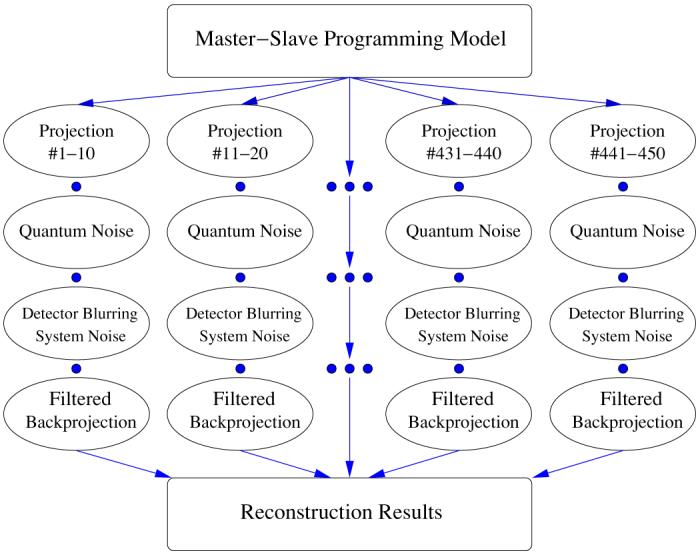
Master–slave parallel programming model.

2.7. Implementation

We now briefly summarize the noise simulation model in the following steps:

(1) Determine I₀ where I₀ is the photon fluence for the open field.

(2) Apply Radon transform formalism to calculate 450 analytical projection image matrices P(i, j) in which each matrix element contains ∑_ku_k × l_k, where u_k is the theoretical linear attenuation coefficient for a specific voxel k and l_k is the passing length, such that the photon fluence I received at each pixel in the flat panel detector is

$$I=I_0{\mathrm{e}}^{-{\sum }_k{u}_k{l}_k}.$$ (13)

(3) Add quantum noise to P(i, j) such that the photon fluence is changed from I to I^′, where

$$I^{\prime }=I_0{\mathrm{e}}^{-{\sum }_k{u}_k{l}_k}+n_q.$$ (14)

Here n_q is a random variable sampled from a Gaussian probability density function. Note that we used the mono-energetic x-ray approach.

(4) Add detector blurring such that

$$I^{″}=I_0\times \frac{I^{\prime }\ast G(x,y)}{I_0\ast G(x,y)},$$ (15)

where G(x, y) is defined in equation (7). Note that I^′ * G(x, y)/I₀ * G(x, y) is for the purpose of normalization.

(5) Add system noise such that

$$I^{‴}=I^{″}+n_s$$ (16)

where n_s is drawn from

$$P\left(x\right)=\frac{1}{\sqrt{2\pi }{\sigma }_s}{\mathrm{e}}^{-\frac{1}{2{\pi }_s^2}}.$$ (17)

Here σ_s denotes the noise level for the system noise, and is determined from the experimental measurement.

(6) Use the Feldkamp filtered backprojection method to reconstruct images as formulated in section 2.5.

2.8. Noise power spectrum (NPS)

The image quality can be evaluated and characterized by measuring the spatial resolution and noise level (Riederer et al 1978). In this paper, the noise power spectra were computed to quantify the noise properties in the reconstructed images. We also used the computed noise power spectra to compare the Ramp and Shepp–Logan filters used in the Feldkamp algorithm.

To determine the parameters in our noise simulation such as the numerical value of σ_s in equation (17), we computed and compared the noise power spectrum in the simulated projection image for the x-ray flat panel detector used in our digital imaging laboratory. For the experimental measurement of the NPS, uniform exposure images were acquired with 120 kVp x-rays filtered by a 0.5 mm thick copper plate and 1.0 mAs setting. The NPS was measured over 100 regions of interest (128 × 128 pixels in each region) that totally occupy an array of 1280 × 1280 pixel area in the central part of the image. A 2D fast Fourier transform (FFT) for each 128 × 128 square region was calculated and the NPS was computed as follows,

$$\mathrm{NPS}(f_x,f_y)=\frac{{\mid \mathrm{FFT}\left\{I(x,y)\right\}\mid }^2}{N_x{N}_y}\times {\Delta }_x{\Delta }_y$$ (18)

where I(x, y) is the projection image data, N_x (N_y) is the number of pixels in the x(y) direction, Δ_x (Δ_y) is the pixel size in the x(y) direction, and f_x (f_y) is the spatial frequency in the x(y) direction. Then we took the average from the upper 4 (y > 0) and lower 4 (y < 0) horizontal lines parallel to the x-axis (y = 0) in the spatial frequency domain (Liu and Shaw 2001, 2004). We used our noise simulation model to calculate the simulated NPS where the parameter σ_s in equation (17) is to be determined and then directly compared to the measurement data where σ_s can be estimated by a statistical method such as chi-square (χ²) statistics (Press et al 1992). Note that the normalized noise power spectra NPS(f_x, f_y)/S² were calculated, where S is the mean image signal.

To evaluate the noise distribution in the spatial frequency space for the reconstructed image, a noise-free image was first reconstructed from an analytical phantom without adding the quantum noise, detector blurring and system noise. Then images from noise-free projection and from projections with added noise were reconstructed and these two images were subtracted from each other. Then a 2D FFT computing routine for the entire 512 × 512 voxel square in the x–y reconstructed image plane at various vertical positions (z = 0.0, 1.0, 2.0, 3.0, 4.0, and 5.0 cm) was performed. The noise power spectra were computed using equation (18) and repeated 500 times to reduce the fluctuation to an acceptable level. In the end, we calculated the average from the 4 upper (y > 0) and 4 lower (y < 0) lines parallel to the x-axis (y = 0) in the spatial frequency domain. The results are presented and discussed in section 3.

3. Results and discussion

3.1. Noise quality test

We compared the Weyl sequence based parallel random number generator to other parallel random number generators by using the visualization technique formulated in section 2.2. Two parallel random number generators selected from the scalable parallel random number generator (SPRNG) library and our implemented Weyl sequence based generator, SNWS, were independently used to reconstruct images from the same analytical projection data and the results are shown in figures 2 and 3. One can easily spot some regular circular patterns in figure 2(b), while no patterns, regular or irregular, are visible in figure 2(a). Also note that various regular circular patterns are present in figure 3(b), while only smooth noisy background is seen in figure 3(a). As mentioned in section 2, we concluded that the Weyl sequence based PRNG results in better randomness and independence than other PRNGs frequently used in Monte Carlo applications. This result is important because it serves to ensure the high quality of the randomness of our noise simulation model (Knuth 1998).

Figure 2.

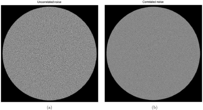
Images reconstructed from data using different parallel random number generators. (a) Uncorrelated noise image: only smooth noisy background is visible. (b) Correlated noise image: regular geometric patterns are visible.

Figure 3.

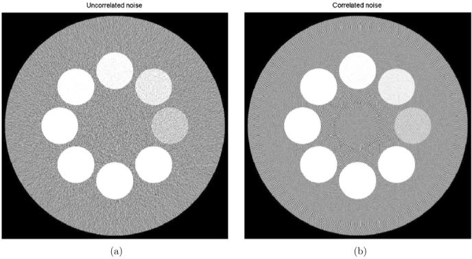
Images reconstructed from data using different parallel random number generators. (a) Image with uncorrelated noise: only smooth noisy background is visible. (b) Image with correlated noise: various circular patterns are visible.

3.2. Noise power spectrum

To determine the best numerical value for the parameter σ_s in equation (17), we computed and compared the noise power spectrum for the simulated projection image for the x-ray flat panel detector. The results from the direct measurement and computer simulation are shown and compared in figure 4. The data were taken from both the experimental measurement (Liu and Shaw 2001, 2004) and the computer simulation. It is clear that these two curves (measurement and simulation) are closely matched. The confidence interval for σ_s was computed to be 95.0% using χ² statistics (Press et al 1992). We then concluded that the parameters used in the noise simulation model for the cone beam CT are well justified.

Figure 4.

Computed NPS for the x-ray flat panel detector. Two curves, one from the experimental measurement and the other one from the computer simulation, are shown simultaneously. Note that the spatial frequency on the x-axis has been rescaled where Nyquist frequency is normalized to 1.0.

In figure 5 we compare the computed noise power spectra at the rotation plane (z = 0.0 cm) for the images reconstructed by using two different filters (Ramp and Shepp–Logan). The result indicated that the Shepp–Logan filter is a better choice over the Ramp filter simply because the noise power spectrum values for the Shepp–Logan filter are lower than the Ramp filter. In figures 6 and 7, we show the computed z-direction dependence for the 2D noise power spectra (z = 0.0 and 5.0 cm) for both the Ramp and Shepp–Logan filters. The results indicated that the overall numerical noise power values decrease when the z value increases for all the spatial frequencies. This characteristic is originated from the Feldkamp reconstruction algorithm because more interpolations are required in the backprojection when the reconstruction plane is not at the plane of z = 0. Mathematically this is equivalent to the smoothing operation (or convolution). Also note that the fan beam reconstruction is performed at the plane of z = 0.

Figure 5.

Computed NPS for the image reconstructed at the mid x–y plane where z = 0. Two curves (one for the Shepp–Logan filter and one for the Ramp filter) are compared. Note that the spatial frequency on the x-axis has been rescaled to where the Nyquist frequency is 1.0 and the y-axis is in logarithmic scale.

Figure 6.

Computed NPS for the images reconstructed at the x–y plane by using the Shepp–Logan filter at z = 0.0 and z = 5.0 cm positions. Note that the spatial frequency on the x-axis has been rescaled to where the Nyquist frequency is 1.0 and the y-axis is in logarithmic scale.

Figure 7.

Computed NPS for the images reconstructed at the x–y plane by using the Ramp filter at z = 0.0 and z = 5.0 cm positions. Note that the spatial frequency on the x-axis has been rescaled to where the Nyquist frequency is 1.0 and the y-axis is in logarithmic scale.

3.3. Applications

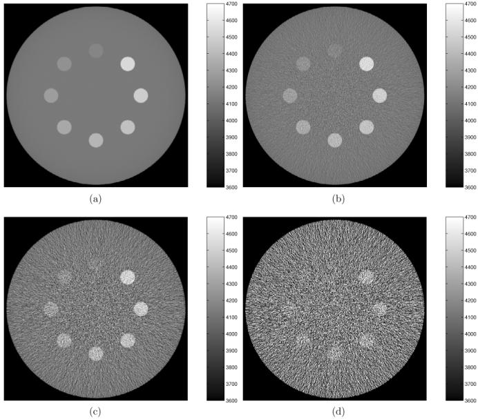
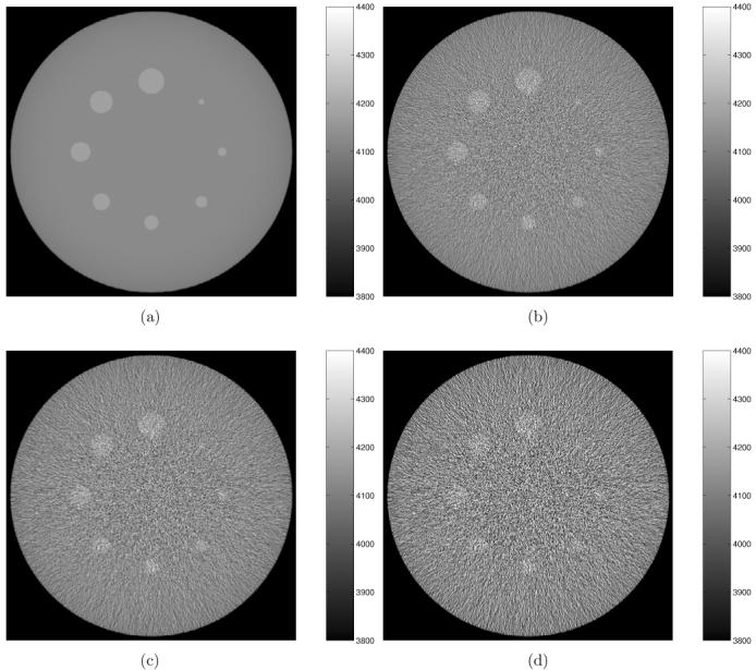
There are several potential applications for our noise simulation model such as a low contrast performance study. In figures 8, 9, 10 and 11, reconstructed images of various mathematical phantoms are shown. They potentially can be used in perception studies for evaluating the low contrast performance of the images. A total of 450 projection views were simulated and the projection image data were obtained by adding the quantum noise, detector blurring and system noise to the analytical computed projections. In figure 8 CBCT images of a 3D phantom simulated with and without the noise are shown. Note that one can do the contrast sensitivity study by varying the noise levels in our noise simulation model. The phantom consists of a cylinder having a diameter of 10.0 cm and a linear attenuation coefficient of 1.0 cm⁻¹ with eight smaller cylinders arranged in a circular manner. The smaller cylinders all have a diameter of 0.8 cm and the attenuation coefficients range from 1.01 to 1.08 cm⁻¹, leading to a contrast level ranging from 1% to 8% relative to the background. In figure 9 a similar phantom contains a big cylinder having a diameter of 10.0 cm and attenuation coefficient of 1.0 cm⁻¹ with eight smaller cylinders of various sizes arranged in a circular manner where the smaller cylinders all have the same attenuation coefficient of 1.01 cm⁻¹ and the diameters range from 0.2 to 0.9 cm. In figure 10 the images of a simulated chest phantom are reconstructed at various simulated stages. The image without adding any noise is shown in figure 10(a). The image with quantum noise is shown in figure 10(b). The image with quantum noise and detector blurring is shown in figure 10(c). The image with quantum noise, detector blurring and system noise is shown in figure 10(d). Note that we are able to show reconstructed images at various independent noise simulated states while in real measurement one can only reconstruct images where quantum noise, detector blurring and system noise have been combined together. In figure 11 we reconstructed the image by using a Gaussian smoothing filter to preprocess the projection data after quantum noise, detector blurring and system noise had been added. The image shows better visual quality if a Gaussian filter is used. Note that all images are shown at the mid x–y plane (z = 0.0) in figures 8, 9, 10 and 11.

Figure 8.

Object visibility versus contrast level. Note that images are shown at the x–y plane when z = 0. Note that the noise level is increasing in the order of (b), (c) and (d). (a) Image reconstructed from analytical projection data (no noise added). (b), (c), (d) Images reconstructed with added noise.

Figure 9.

Object visibility versus size. Note that images are shown at the x–y plane when z = 0. Note that the noise level is increasing in the order of (b), (c) and (d). (a) Image reconstructed from analytical projection data (no noise added). (b), (c), (d) Images reconstructed from projection image data with noise added.

Figure 10.

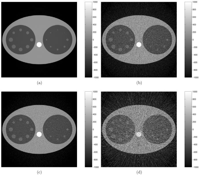
Reconstruction images shown at various simulated stages. Note that images are shown at the x–y plane where z = 0. (a) Image reconstructed from analytical projection data. (b) Image with only quantum noise simulated. (c) Image with quantum noise and detector blurring simulated. (d) Image with quantum noise, detector blurring and system noise simulated.

Figure 11.

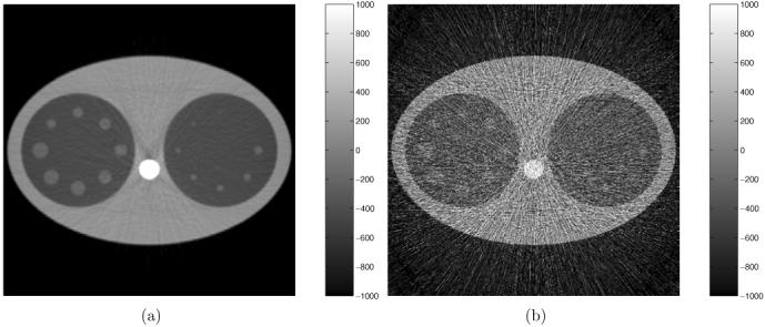
Reconstructed images in which quantum noise, detector blurring and system noise are all simulated. In this specific case, the image reconstructed with a pre-filtering process shows better image quality than the image without a pre-filtering process. Note that the same phantom is used as in figure 10 and the image is shown at the x–y plane where z = 0. See the text for details. (a) Image reconstructed with a pre-filtering process. (b) Image reconstructed without a pre-filtering process.

4. Conclusions

We have presented a parallel simulation model and developed a software tool to incorporate quantum noise, detector blurring and system noise in cone beam computed tomography imaging. A correlation-free parallel random number generator based on the Weyl sequence was implemented, tested and compared with other parallel random number generators. A visualization technique was also developed to detect the non-random patterns hidden in the parallel random number generators, and the results showed that our implemented generator delivered better quality than the other tested generators. Two different filters, the Ramp and the Shepp–Logan filter, used in the Feldkamp reconstruction algorithm were compared and the dependence on the z direction at the reconstruction x–y plane for the noise power spectrum was also evaluated. In the end, we demonstrated that our developed noise simulation model can be used for the purpose of contrast-detail study by creating mathematical phantoms for specific imaging scenarios and generating reconstructed images corresponding to various imaging techniques or conditions.

References

- Ackermann J, Tangen U, Bodekker B, Breyer J, Stoll E, McCaskill JS. Comput. Phys. Commun. 2001;140:293–302. [Google Scholar]
- Bushberg J, Seibert J, Leidholdt E, Boone J. The Essential Physics of Medical Imaging. 2nd edn Lippincott Williams & Wilkins; Philadelphia, PA: 2002. [Google Scholar]
- Chen ZK, Ning RL. Phys. Med. Biol. 2004;49:1865–80. doi: 10.1088/0031-9155/49/10/003. [DOI] [PubMed] [Google Scholar]
- Cheng QH, Cao L, Wu DJ. Acta Phys. Sin. 2004;53:2556–62. [Google Scholar]
- Chesler DA, Riederer SJ, Pelc NJ. J. Comput. Assist. Tomogr. 1977;1:64–74. doi: 10.1097/00004728-197701000-00009. [DOI] [PubMed] [Google Scholar]
- Entacher K, Uhl A, Wegenkittl S. Lecture Notes in Computer Science. Vol. 1557. Springer; Berlin: 1999. Parallel Computation; pp. 107–16. [Google Scholar]
- Faulkner K, Moores BM. Phys. Med. Biol. 1984;29:1343–52. doi: 10.1088/0031-9155/29/11/003. [DOI] [PubMed] [Google Scholar]
- Feldkamp LA, Davis LC, Kress JW. J. Opt. Soc. Am. 1984;A 1:612–9. [Google Scholar]
- Granfors PR, Aufrichtig R. Med. Phys. J. 2000;27:1324–31. doi: 10.1118/1.599010. [DOI] [PubMed] [Google Scholar]
- Hahn LJ, Jaszczak RJ, Gullberg GT, Floyd CE, Manglos SH, Greer KL, Coleman RE. Phys. Med. Biol. 1988;33:541–55. doi: 10.1088/0031-9155/33/5/003. [DOI] [PubMed] [Google Scholar]
- Hampton C, Munley M, Bourland J. Med. Phys. 2003;30:1474. [Google Scholar]
- Holian BL, Percus OE, Warnock TT, Whitlock PA. Phys. Rev. 1994;E 50:1607–15. doi: 10.1103/physreve.50.1607. [DOI] [PubMed] [Google Scholar]
- Kak AC, Slaney M. Principles of Computerized Tomographic Imaging. Society for Industrial and Applied Mathematics; Philadelphia, PA: 2001. [Google Scholar]
- Kijewski MF, Moore SC, Mueller SP, Holman BL. J. Nucl. Med. 1991;32:899. [Google Scholar]
- Knuth DE. The Art of Computer Programming. 3rd edn Vol. 2. Addison-Wesley; Reading, MA: 1998. [Google Scholar]
- Koniges AE, Leith CE. J. Comput. Phys. 1989;81:230–5. [Google Scholar]
- Laforenza D. Lecture Notes in Computer Science. Vol. 3112. Springer; Berlin: 2004. Towards a Next Generation Grid. [Google Scholar]
- Liang YF, Whitlock PA. Math. Comput. Simul. 2001;55:149–58. [Google Scholar]
- Liu XM, Shaw CC. Med. Phys. 2001;28:1080–92. doi: 10.1118/1.1376136. [DOI] [PubMed] [Google Scholar]
- Liu XM, Shaw CC. Med. Phys. 2004;31:98–110. doi: 10.1118/1.1625102. [DOI] [PubMed] [Google Scholar]
- Logan BF, Shepp LA. Duke Math. J. 1975;42:645–59. [Google Scholar]
- Maolinbay M, El-Mohri Y, Antonuk LE, Jee KW, Nassif S, Rong X, Zhao Q. Med. Phys. 2000;27:1841–54. doi: 10.1118/1.1286721. [DOI] [PubMed] [Google Scholar]
- Marchenko MA, Mikhailov GA. Russ. J. Numer. Anal. Math. Modelling. 2002;17:113–24. [Google Scholar]
- Mathews J, Walker RL, Joint A. Mathematical Methods of Physics. 2nd edn Benjamin; New York: 1970. [Google Scholar]
- Mueller K, Yagel R. IEEE Trans. Med. Imaging. 2000;19:1227–37. doi: 10.1109/42.897815. [DOI] [PubMed] [Google Scholar]
- Ning R, Tang XY, Conover D. Med. Phys. 2004;31:1195–202. doi: 10.1118/1.1711475. [DOI] [PubMed] [Google Scholar]
- Parry M, Fischbach E. J. Math. Phys. 2000;41:2417–33. [Google Scholar]
- Press WH, Vetterling WT, Flannery BP, Teukolsky SA. Numerical Recipes in C: The Art of Scientific Computing. 2nd edn Cambridge University Press; Cambridge: 1992. [Google Scholar]
- Press WH, Vetterling WT, Flannery BP, Teukolsky SA. Numerical Recipes in FORTRAN 90: The Art of Parallel Scientific Computing (Fortran Numerical Recipes v.2) 2nd edn Cambridge University Press; Cambridge: 1996. [Google Scholar]
- Quinn MJ. Parallel Programming in C with MPI and OpenMP. McGraw-Hill; Boston: 2004. [Google Scholar]
- Riederer SJ, Pelc NJ, Chesler DA. Phys. Med. Biol. 1978;23:446–54. doi: 10.1088/0031-9155/23/3/008. [DOI] [PubMed] [Google Scholar]
- Saarinen J, Tomberg J, Vehmanen L, Kaski K. IEE Proc. 1991;E 138:138–46. [Google Scholar]
- Schleef D, Parry M, Tu SJ, Woodahl B, Fischbach E. J. Math. Phys. 1999;40:1103–12. [Google Scholar]
- Smith BD. Opt. Eng., Bellingham. 1990;29:524–34. [Google Scholar]
- Srinivasan A, Mascagni M, Ceperley D. Parallel Comput. 2003;29:69–94. [Google Scholar]
- Tretiakov KV, Wojciechowski KW. Phys. Rev. 1999;E 60:7626–8. doi: 10.1103/physreve.60.7626. [DOI] [PubMed] [Google Scholar]
- Tu SJ, Fischbach E. J. Phys. A: Math. Gen. 2002;35:6557–70. [Google Scholar]
- Tu SJ, Fischbach E. Phys. Rev. 2003;E 67:016113. doi: 10.1103/PhysRevE.67.016113. [DOI] [PubMed] [Google Scholar]
- Tu SJ, Shaw CC, Chen L. Med. Phys. 2004;31:1821. [Google Scholar]
- Wilkinson B, Allen CM. Parallel Programming: Techniques and Applications Using Networked Workstations and Parallel Computers. 2nd edn Pearson; Upper Saddle River, NJ: 2005. [Google Scholar]