HotPatch: A Statistical Approach to Finding Biologically Relevant Features on Protein Surfaces

Abstract

We describe a fully automated algorithm for finding functional sites on protein structures. Our method finds surface patches of unusual physicochemical properties on protein structures, and estimates the patches’ probability of overlapping functional sites. Other methods for predicting the locations of specific types of functional sites exist, but in previous analyses, it has been difficult to compare methods when they are applied to different types of sites. Thus, we introduce a new statistical framework that enables rigorous comparisons of the usefulness of different physicochemical properties for predicting virtually any kind of functional site. The program’s statistical models were trained for 11 individual properties (electrostatics, concavity, hydrophobicity, etc.) and for 15 neural network combination properties, all optimized and tested on 15 diverse protein functions. To simulate what to expect if the program were run on proteins of unknown function, as might arise from structural genomics, we tested it on 618 proteins of diverse mixed functions. In the higher-scoring top half of all predictions, a functional residue could typically be found within the first 1.7 residues chosen at random. The program may or may not use partial information about the protein’s function type as an input, depending on which statistical model the user chooses to employ. If function type is used as an additional constraint, prediction accuracy usually increases, and is particularly good for enzymes, DNA-interacting sites, and oligomeric interfaces. The program can be accessed online at http://hotpatch.mbi.ucla.edu.

Introduction

When a protein’s structure is first solved, it is generally examined for unusual features likely to be functionally important, such as clefts^1,2, patches of certain chemical or structural properties^3,4, possible catalytic residues⁵, or exposed conserved residues^6,7. Searching for structural insights into functional mechanisms is the most common means by which we exploit our understanding of structure-function relationships.

The assessment of functional relevance from structural data is still most often guided by experience, and is rarely quantitative, even amidst the bioinformatics revolution. Our substantial knowledge of protein structure/function relationships is applied to practical problems via techniques that, for the most part, remain piecemeal and comparatively subjective. In contrast, bioinformatics has attacked genomic sequence analysis with large-scale computational methods like Psi-BLAST⁸, PROSITE^9,10, PRINTS¹¹ and Pfam¹².

Meanwhile, structural genomics initiatives (SGI) promise to deliver a great acceleration in the current rate of protein structure determination^13,14,15,16, providing an opportunity to use bioinformatic methods in structure analysis. It also creates new challenges, as it will be increasingly common for structures to be solved with unknown functions and/or novel folds^{17,18,19,20,21,22}. There will be an increasing need for automated methods to identify types of functions and locations of functional sites from protein structures^18,19,20,21.

Towards this end, sequence conservation information is often mapped onto protein structures. Sequence-based methods for finding functional residues require a collection of homologs with reasonable sequence diversity, or the presence of common sequence motifs^9,10. Methods have been developed to automatically search for clusters of conserved residues on structures^6,7,23,24. This approach can be challenging, because functional residues may not be conserved within a family if sub-families have different functions or different specificities. One method, Evolutionary Trace^7,25, attempts to exploit both sequence conservation and subfamily variation, but is hard to automate. Sequence analysis will continue to be important, but if the sequence family is too small, too diverse, or not diverse enough, it can be difficult to find functional residues this way.

It is sometimes possible to guess the locations of functional sites on a structure by comparing it to others of a similar fold, but there are many examples of proteins that share the same fold, but have very different functions^26,27,28.

Methods to identify functional sites directly from structure have also been developed. Perhaps the most common approach is to find a large cleft or pocket, a task automated by several algorithms^29,30,31,32. These methods often report that an active site is inside the largest cleft in ~80–90% of a test set of enzymes^2,30,31. Though important, these methods have some limitations. First, the largest cleft is usually several times larger than the active site, so such predictions are not very specific. Second, they are intended mainly for enzyme analysis, while about 50% of structures in PDB have no catalytic site. And third, some types of interactions, like protein binding, usually occur outside concavities³.

To predict protein-protein interaction sites, several methods identify patches of hydrophobicity^4,33,34 or patches of planar shape³⁴. Residue-residue interaction propensities^35,36,37 have been used to study protein-protein interactions, and for discriminating dimer interfaces from crystal contacts³⁸. To predict enzyme active sites, other methods use structural (3-D motif) matching against known sites^{19,22,39,40,41,42,43,44,45}. Electrostatic destabilization was used to predict the active sites of six enzymes⁴⁶. Ionizable residues, whose computed charges were independent of pH variation, were used to predict catalytic residues on three enzymes⁴⁷. To predict metal ion-binding sites, one method finds atom clusters high in ‘hydrophobic contrast’⁴⁸. In general these methods judged their success rates by different criteria, which were applied to different test sets that varied widely in size and type, making comparisons between them difficult.

The methods cited above are quite diverse, but most share three features. First, most of them look for clusters of residues that share some property in 3-D space. Second, the properties are often chosen based on intuition rather than a rigorous evaluation of their usefulness for a particular function. Third, most of them predict a region to be functional, but do not estimate the likelihood of success.

Numerous methods exist for predicting the functional types of proteins of unknown function, and other methods for predicting functional sites on proteins of known function. But it is particularly difficult to predict functional sites on proteins of totally unknown function; yet exactly this type of problem will result from structural genomics.

Here we describe an automated algorithm, HotPatch, for predicting the locations of functional sites by finding patches of unusual properties on protein surfaces. The method differs from previous efforts in four ways. First, the program computes, for each patch, a statistical estimator representing the probability that the patch overlaps a functional site. This statistic, called Functional Confidence, is a “quality factor” by which we may judge the reliability of the prediction. It is analogous to statistical estimators of homology returned by sequence analysis programs, like Psi-BLAST’s p-value⁸. Functional confidence makes it practical to use HotPatch on proteins of known or unknown functional type, by extracting only those predictions that are most reliable.

Second, our method is optimized to predict very specific patches, where specificity is defined as the fraction of residues in the predicted region that are functional. Other methods, like those that find the largest cleft, often overpredict, identifying regions larger than the functional site. Specific predictions are more useful to experimentalists, because they minimize the work they must do, e.g. when introducing mutations to test a predicted site, or when designing a site inhibitor.

Third, HotPatch treats oligomers in their biologically relevant quaternary structure. Most previous methods have restricted their analysis to monomers only, or have treated single subunits of oligomers as if they were monomers. Thus, functional sites shared between subunits (which are common) were either avoided or analyzed inaccurately.

Fourth, the approach is general. The property analyzed can be any smoothly varying local property of proteins, such as hydrophobicity, electrostatic potential, or a combination via a neural network. The functional site can be of unknown type, or of any known type, assuming there is a set of example structures on which HotPatch can be trained. When the user chooses to predict sites with a statistical model trained on a specific function, partial information about the function type is in effect an additional input. But when the user chooses a statistical model trained on a mixture of functions, the test protein’s function type need not be known ahead of time. In these cases we have decoupled the problem of functional site prediction from the problem of function type prediction. (For comparison, sequence conservation methods sometimes require no knowledge of function (e.g. BLAST), while other conservation methods (e.g. Evolutionary Trace) require detailed knowledge of the test protein’s function.)

The generality of our method and of our statistical framework allow us to rigorously compare the usefulness of 11 individual physicochemical properties, plus 15 Neural Network combination properties, all optimized for predicting 15 diverse types of functional sites.

Results and Discussion

To predict functional sites, HotPatch performs the following steps: 1. it evaluates the property of interest (individual property or Neural Network combined property) for all atoms in the protein; 2. it clusters together atoms with high values of the property; and 3. to each patch, it assigns a statistical score called Functional Confidence (FC, see Table 1 for abbreviations) describing how probable it is for the patch to overlap a functional site.

Table 1.

Definitions of Statistical Terms

Acronym	Long Name	Equ. #
speck sensk FC FFSR RCUS	specificity of patch k sensitivity of patch k Functional Confidence Fraction of Functional Surface Residues Residue Count Until Success	1 S2 (Supplement) S3 (Supplement) 2 5

Example of HotPatch Predictions

Before reporting accuracy statistics for all of HotPatch’s predictions, we first show a few examples of what the site predictions look like. Of the 15 protein functions examined in the current work, we focus first on our generic function test set (see below), a mix of all protein functions. Predictions with this set assume no knowledge of the type of function, simulating a “worst case scenario” as might be encountered in Structural Genomics. Of the 11 properties analyzed by HotPatch, for illustrative purposes we begin with examples using electrostatic potential. (Note the Neural Net is a better predictor than electrostatics by itself.) Although electrostatic potential is not useful for all function types, we can use HotPatch’s Functional Confidence (FC) as a “quality factor” to tell us when the program has confidence this property is useful for predicting a site of unknown type.

From predictions for the 618 proteins in this set of structures, the first six with the highest FC’s are shown in Fig. 1.a–f. The selection of these six involved no a priori knowledge of prediction success, only their FC’s. For each structure, Fig. 1 shows the top two (or three, in 1.b) predicted hotpatches of electrostatic potential, displayed alongside the functional sites. (See Supplementary Materials for details on the proteins, their functions and predicted residues.) The fraction of residues that are functional (i.e. specificities, see Eq. 1) in the #1 high-scoring patches on the six proteins are 80%, 83.3%, 68.4%, 87.5%, 65%, and 85%. For their #2 patches, the specificities are 0%, 100%, 60%, 100%, 70%, and 100%. Among the enzymes, the #1 patches all include one or more catalytic residues. Although we only illustrate the top six proteins, in this test set, the #1 patch overlaps a site with specificity ≥ 1/3 in the top 21 proteins with the highest FC’s.

Figure 1.

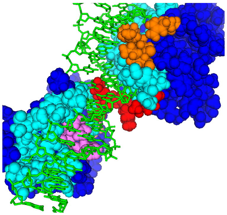
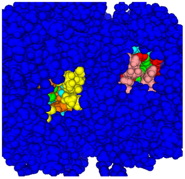
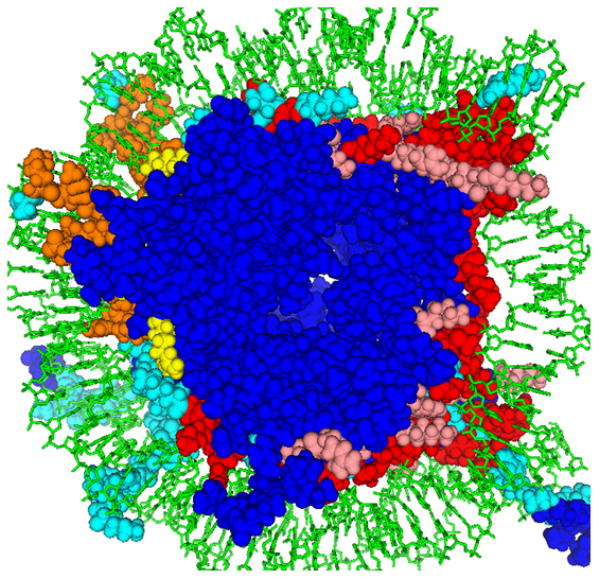
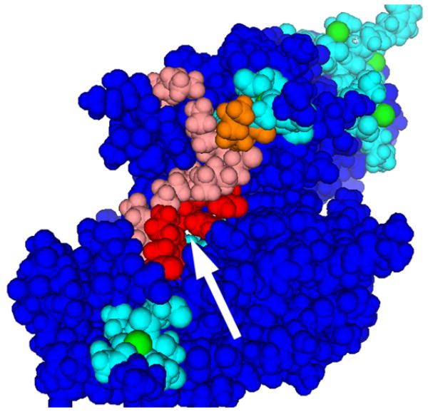
Examples of functional sites predicted using patches of electrostatic potential. The first six structures (a.–f.) have the highest FC’s from the generic function subset. The color scheme used is: red (or orange) = in patch #1 (or #2) and also in functional site, i.e. correct prediction; pink (or yellow) = in patch #1 (or #2) but not in functional site, i.e. overprediction; cyan = in functional site but not in patch #1 or 2; green = substrate (if present). a. Uroporphyrinogen decarboxylase (pdb 1URO). b. DNA-binding domains of RAP1 (pdb 1IGN); patch #3 is in violet. c. Alanine racemase (pdb 1BD0). d. Uridylyltransferase (pdb 1GUP). e. Nucleosome core particle (pdb 1AOI). f. Annexin III (pdb 1AXN); arrow points to putative channel entrance.

Several of the proteins are large complex oligomers, e.g. the nucleosome core particle (Fig. 1.e). Two proteins (Fig. 1.c,d) have active sites shared between subunits, sites that probably would not be found by other algorithms that treat oligomers as monomers. On Annexin III (Fig. 1.f), the membrane binding sites are not precisely known, but the #1 patch is found in a sequence-conserved region at a channel entrance, thus predicting an unknown binding site, and supporting theories that this region is a calcium channel⁴⁹.

The six proteins shown in Fig. 1 are diverse—two bind DNA, one binds membranes, and three are enzymes of distinct classes—but for most, the substrate is partially negatively charged (not surprising, as the property used is electrostatic). Thus, a high FC is not restricted to one functional type, but does provide hints at the nature of the interaction.

Example of a Pharmacologically Relevant HotPatch Prediction

Caspases are critical mediators of apoptosis and the inflammatory response, and are an important class of drug targets for stroke, cancer, and inflammatory disease. The highly specific nature of caspase active sites have so far frustrated drug discovery efforts. An alternative possibility is to influence their regulation by targeting an allosteric site. Traditionally it has been difficult to identify novel allosteric sites, however. As described in Hardy et al.⁵⁰, a previously unreported allosteric regulatory site was predicted by HotPatch. The #1 patch of concavity is buried between two subunits of the dimer, as shown in Fig. 1 of Hardy et al.⁵⁰ Compounds that target this allosteric site were found to inhibit the enzyme and prevent peptide binding at the active site.

The active site is not concave, however, and was not found by patches of concavity. We analyzed caspase-7 (pdb 1I51) using electrostatics. The #1 patch of electrostatic potential (FC = 48%) overlaps the active site, and includes both catalytic residues (H144, C186).

The above examples showed HotPatch predictions with high Functional Confidence scores for the generic function test set analyzed by electrostatic potential. Below we assess HotPatch predictions for many protein functions analyzed by many properties.

Protein Functions and Physical Properties Analyzed

HotPatch’s statistical models were trained against subsets of proteins of the same function, extracted from the SFR database of known functional sites [http://nih.mbi.ucla.edu/~pettit/sfr]. The subsets, described in Table 2, consist of several catalytic types (e.g. protease, abbreviated pr, hydrolase abbreviated hy, etc.), some non-catalytic types (protein-binding pb, oligomeric interface ol), and some defined by type of substrate (e.g. positive metal ion-binding mp). Subsets pb and ol distinguish between transient protein-binding interfaces and constitutively bound oligomeric interfaces. Catalytic generic (cg) includes all enzyme types. Its site residues are defined by annotation (in SFR) or by proximity to a substrate in a complex; thus they are involved in catalysis and/or substrate binding. The other enzyme types (hydrolase, transferase, etc.) are specific subsets of cg, and likewise consist of mixed catalytic/binding/recognition residues. Subsets vary in size from 618 proteins (for generic function) to 24 (proteases).

Table 2. Functional Subsets of Proteins.

Abbreviations and sizes of subsets of proteins with particular functions as extracted from the SFR Database. Site Definition describes how functional residues were defined: “notes” means by residue annotations in SFR, “prox.” means by proximity of 4 Å to a substrate or mimic of a substrate in structures of complexes. FFSR = fraction of functional residues on protein surface (see Eq. 2). (Numbers in parentheses are for structures with hydrogens added, used for electrostatic & neural net computations.)

Abbrev	Long Name	Catalytic	Site Defn.	FFSR	# Proteins
gf	generic function	Y/N	notes/prox.	0.127 (0.139)	618 (597)
ol	oligomeric interface	N	prox.	0.280 (0.302)	328 (327)
pb	protein-binding	N	notes/prox.	0.149 (0.156)	146 (145)
pr	protease	Y	notes/prox.	0.096 (0.116)	24 (23)
hy	hydrolase	Y	notes/prox.	0.084 (0.092)	103 (101)
ki	kinase	Y	notes/prox.	0.102 (0.110)	25 (23)
tr	transferase	Y	notes/prox.	0.095 (0.103)	70 (67)
or	oxidoreductase	Y	notes/prox.	0.087 (0.099)	91 (83)
cg	catalytic general	Y	notes/prox.	0.087 (0.096)	312 (295)
dn	DNA/RNA-interacting	Y/N	notes/prox.	0.153 (0.165)	114 (113)
in	negative ion-interacting	Y/N	notes/prox.	0.049 (0.052)	41 (39)
sm	small molecule-interacting	Y/N	notes/prox.	0.075 (0.083)	246 (229)
cm	carbohydrate-interacting	Y/N	notes/prox.	0.062 (0.070)	61 (59)
lp	lipid-interacting	Y/N	notes/prox.	0.060 (0.066)	40 (39)
mp	positive metal ion-binding	Y/N	notes/prox.	0.041 (0.050)	165 (152)

Two subsets are especially relevant to structural genomics initiatives: catalytic generic (cg), and generic function (gf), a mix of all kinds of functional sites. When these more generic subsets are used for training, little or nothing need be known a priori about the function type of the test protein. But when the user of HotPatch chooses to predict sites using the more specific function subsets above, function type is in effect an input.

We analyzed HotPatch’s site predictions using 11 physical properties. Electrostatic potential⁵¹ and charge⁵² (positive and negative) and surface roughness⁵³ are abbreviated as epotn, negepotn, poscharge, negcharge and rufness. Concavity was assessed in two ways: by an algorithm similar to Connolly’s⁵⁴, and by the program CAST⁵⁵, abbreviated as concav and castcav. Hydrophobicity and hydrophilicity were defined on a by-residue⁵⁶ or by-atom⁵⁷ basis, abbreviated as hydrofob.res, hydrofil.res, hydrofob.at and hydrofil.at. Below we present results of testing 11 individual properties on 15 protein functions, for 164 combinations (not 165 because we did not test castcav for subset ol; see Methods).

In addition we designed neural networks^58,59,60,61 that combine all above properties with other properties (e.g. residue exposed area) together into ‘super-predictor’ properties. Each neural network (NN) is optimized and tested on one of the 15 protein functions, e.g. the NN optimized for hydrolases is only tested on hydrolases. For all properties, individual or NN, the overfitting of data is prevented by a jackknifing technique.

Estimation of Functional Confidence

In the examples above, we used high FC values to extract successful predictions from a large data set. However, Functional Confidence is more than just a quality factor; it has a useful statistical interpretation. To define FC, we assume patches can be ordered by some value, like patch size or score. The Functional Confidence of patch k is defined as the probability that a patch of its size (or larger) will successfully overlap a functional site, given that at least one patch of its size (or larger) exists on the protein. The overlap of a patch and site is the fraction of functional residues in the patch (i.e. its specificity):

$$\mathit{spe}{c}_k=\frac{a_k}{b_k}$$ (1)

where b_k is the number of residues in patch k, and a_k is the number of residues that are both in patch k and in the site. In defining FC, “successful overlap” means that the patch specificity exceeds a fixed percentage. In the current work we set the specificity cutoff somewhat arbitrarily at 1/3. Of course other cutoffs are possible, and success criteria vary widely in the literature. (In Supplementary Materials we give a mathematical expression for FC). The FC of a patch obviously can only be defined if a protein has at least one patch of that size. HotPatch estimates FC for patch k, by comparing against a training subset of proteins with known sites, that all have at least one patch the size of k or larger.

The six examples above showed HotPatch predictions with high FC that overlapped functional sites. Is this is true in general, i.e. is the actual rate of successful overlaps for patches generally higher when their FC is higher, and lower when their FC is lower? As it is impractical to display all 164 property-function combinations tested here, for a few interesting combinations we plot actual success rates vs. estimated FC’s in Fig. 2. On the x axis, the #1 patches from all proteins in the test set are binned by their estimated FC’s. The y axis shows fractions of successful #1 patches in each FC bin, and a linear fit to the success rate. Ideally, the success ratio vs. estimated FC should be a diagonal. The success ratios are jagged due to small counts in some bins, but there is a clear upward trend.

Figure 2.

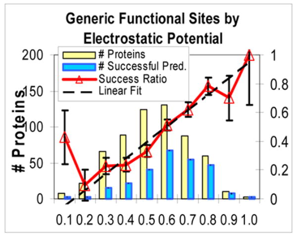
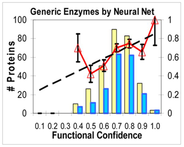
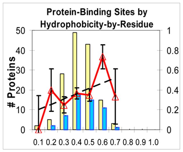
Rate of successful predictions vs. estimated Functional Confidence (FC) for some properties and functions of interest. x axis: for a large set of proteins of the same function, the estimated FC values of their #1 high-scoring patches were binned in intervals of 0.1. On the y axis: thick line with triangles: ratio of successful predictions in each bin (ideally, should be diagonal). Light bar: count of #1 patches that had an estimated FC in that bin. Dark bar: count of #1 patches in that bin that successfully overlapped a functional site. Dashed line: linear fit to unbinned success rate data. In Figs 2.a–f, the fits have slopes 1.11, 0.72, 0.67, 0.69, 0.53, and 0.65. a. Generic functional sites (all functions) by electrostatic potential. b. DNA/RNA-interacting sites by electrostatic potential. c. General catalytic sites by Neural Net combination property. d. Oligomeric interfaces by hydrophobicity. e. Protein-binding sites by hydrophobicity. f. (negative control) DNA/RNA-interacting sites by hydrophobicity.

Figs 2.d, e, and f are all for one property (hydrophobicity) but for three types of sites, that are strongly correlated, weakly correlated, and anti-correlated with hydrophobicity. As the protein function is less correlated with the property, actual success rate goes down and FC goes down, so the distribution shifts from high to low and from right to left. Fig. 2.f, a negative control (DNA/RNA-interacting sites by hydrophobicity), shows that low FC’s emitted by HotPatch can be a reliable warning when a property is a poor predictor for a given function. Also, in Supplementary Materials we present receiver-operator characteristic (ROC) curves that further show the reliability of FC estimation.

The above results show that predictions with high FC’s are more likely to overlap sites. However, for some function-property combinations, patches with high FC’s may occur rarely, since each physical property is useful for some functions but not for others. Thus we must address two important questions. First, which properties are most useful for each protein function? Second, for the best properties of each function, how often on average do high-FC patches produce useful predictions?

Measuring Usefulness of Site Predictions With Two New Statistics

To be useful, a property must produce successful predictions in many proteins. However, there is no universally accepted measure of usefulness for site prediction methods. Thus we introduce two statistics to quantify the usefulness of site predictions. One statistic, success rate, gauges the usefulness of the #1 high-scoring patch. The second, Residue Count Until Success (RCUS), considers all (high and low-scoring) patches.

Success rate is the percent of proteins whose #1 patch has specificity above a threshold (set arbitrarily at ≥ 1/3, as above, with specificity defined in Eq. 1); e.g. for a patch of ten residues, four or more functional residues mean a “success”, while three mean a “failure.” Fig. 3 graphically displays success rates for the #1 patches of all properties, averaged over all proteins in each function subset. These values, with no FC cutoff, give an overview of which properties are most useful for each function. For a given function (column in Fig. 3), the best success rate among all properties (with no FC cutoff) varies from 40% (for protein-binding) to 78% (for oligomeric interfaces and proteases).

Figure 3.

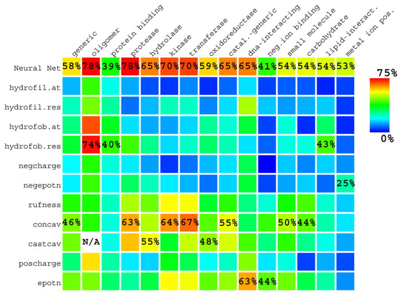
Success rates of the #1 high-scoring patch on each protein, averaged over all proteins in all functional subsets (with no FC cutoff) for all properties. Here “success” means #1 patch specificity ≥ 1/3. Besides annotating success rates for the Neural Networks, in each protein function (column) the second highest success rate (excluding the NN) is also annotated. Oligomeric interfaces were not evaluated by CAST concavity (castcav).

The large variations seen between different protein functions are partially due to large variations in the sizes of their sites. It is easy to predict the location of a big site on a small protein, but hard for a small site on a big protein. When comparing accuracies between functions, we take into account the relative difficulty of predicting sites of different sizes, by defining the Fraction of Functional Surface Residues (FFSR):

$$\mathit{FFSR}=\frac{\#\hspace{0.17em}\text{functional\hspace{0.17em}site\hspace{0.17em}residues}}{\#\hspace{0.17em}\text{surface\hspace{0.17em}residues\hspace{0.17em}on\hspace{0.17em}protein}}$$ (2)

Table 2 lists FFSR’s averaged over each subset. The easiest subset to predict is oligomer interface (ol), and the hardest is metal ion-binding (mp), with FFSR’s = 0.28 and 0.041.

Although success rate is useful for comparing physical properties for prediction, it depends on an arbitrary overlap criterion of 1/3. For example, a #1 patch of seven residues in which two residues are functional is designated a failure. Moreover, sometimes when the #1 patch has failed, the #2, #3 patches etc., may succeed. Incorporating these results can be complex, because average patch sizes vary widely.

We therefore introduce a second, simplifying statistic to measure usefulness, called Residue Count Until Success (RCUS). This takes into account all patches on a protein, and also accounts for semi-successful patches with specificity greater than zero but < 1/3. RCUS estimates how many residues an experimentalist might need to test (by, e.g., site-directed mutagenesis, labeling, etc.) before finding one functional residue. For example, if a patch had five residues, of which one was functional, and if an experimentalist picked at random from it, she might find a functional residue after picking one, or sometimes after picking five; but on average she would pick three. To generalize: if an algorithm predicts a set of regions (here, patches) ordered by a criterion (here, FC), and if we initially choose residues at random from the first patch, and secondly at random from the second patch, etc., and lastly from the non-patch surface, then RCUS is the mean number chosen until we find at least one functional residue. Obviously, a smaller RCUS is better.

Table 3 lists the median RCUS for each protein function (with no FC cutoff). These values should be compared against RCUS_RAN, the mean number of residues that would be chosen at random from the whole protein surface (typically 9–12, sometimes much higher). Equations for RCUS and RCUS_RAN are given in Methods. (In Supplementary Materials we tabulate more statistics, such as mean specificities, sensitivities, etc.)

Table 3. Median RCUS and RCUS_RAN over all proteins (with any FC).

The properties listed are the two best properties for each protein function. RCUS (Residue Count Until Success) of a prediction and RCUS_RAN (the RCUS expected for a random predictor) are defined in Eqs. 5 and 4 respectively.

Function	Property	RCUS	Random RCUS
generic	NN	2	9.6
	epotn	3	7.9
	concavity	2.5	8.4
oligomeric interface	NN	1.5	4.1
	hydrofob	1.4	4.1
protein-binding	NN	4.0	8.4
	hydrofob	3.5	8.3
protease	NN	1.4	11.8
	concavity	1.2	8.9
	rufness	2.5	8.9
hydrolase	NN	1.7	13.3
	concavity	2	11.5
	rufness	2.8	11.5
kinase	NN	1.8	9.7
	concavity	2	8.5
	epotn	2.7	8.5
transferase	NN	1.8	10.6
	concavity	1.7	9.4
	epotn	2	8.9
oxidoreductase	NN	2.1	12
	epotn	3.3	9.4
	concavity	3	9.1
catalytic general	NN	1.8	12.5
	epotn	3	9.8
	concavity	2.2	10.7
DNA/RNA interacting	NN	1.8	7.8
	epotn	1.7	7.4
	hydrofil	2.5	7.4
negative ion binding	NN	3.2	21.8
	epotn	5	19.2
	concavity	3.5	18
smallmolecule	NN	2.3	14.1
	epotn	3.5	12.4
	concavity	2.5	13.8
carbohydrate	NN	2	15.4
	epotn	6	14.4
	rufness	5	12.9
lipid-Interacting	NN	2.4	17.3
	hydrofob	6.5	16.3
	epotn	7	15.5
metal pos. ion binding	NN	2	36.3
	negepotn	10.8	23.9
	concavity	14.4	27.9

Which Properties are Most Useful for Each Protein Function?

By comparisons of the usefulness of diverse properties for diverse protein functions, novel structure-function relationships can be discovered. Of the 164 function-property combinations displayed in Fig. 3, we briefly summarize which properties are useful for predicting sites of each type. In evaluating which physical properties will be the best site predictors, we assume we know the protein function type a priori. Below we distinguish between useful function-property combinations that are to be expected from previously well-known principles, and useful combinations that are novel and unexpected. Of properties previously known to be useful, the most well-known are hydrophobicity for oligomeric interfaces^4,33,34 and concavity for enzyme sites^2,29,30,31.

We found electrostatic potential useful for many functions: generic sites, most enzyme sites, and several kinds of substrate binding sites. Some of these uses for electrostatics are well-known (e.g. for predicting DNA-binding sites^62,63). However, the use of electrostatic potential by itself to predict enzyme sites has, to our knowledge, not been reported. We found it useful for a mix of all enzyme sites, for transferases and for oxidoreductases.

We also find electrostatic potential always more useful than electric charge; and hydrophobicity more useful as defined by-residue than by-atom (i.e. by ASP⁵⁷). The only enzymes for which hydrophobicity works are the proteases, and that is marginal (success rate of 42% over all FC). Because the protease subset is small, this result is tentative.

We previously showed that surface roughness is useful for small molecule binding sites⁵³. The novel results here are that we find it moderately useful for all enzyme types and for all types of substrate binding sites (usually as the third best property).

The statistics in Fig. 3 and Table 3 are evaluated over all proteins, but in practice, only proteins with FC above a reasonable threshold would be considered actual predictions. Which threshold is reasonable depends on the protein function, however, because the difficulty of prediction (FFSR) varies. For example, in the DNA/RNA-interacting subset, there are many electrostatic patches with FC above 0.70, but in some functions that are harder to predict, no patch has FC > 0.70. Thus, for each function-property combination, we fixed a success rate and found the FC threshold at which that success rate is achieved. The percentage of all proteins with a patch FC above the threshold (the coverage) must be significant for that property to be useful for that function. For three fixed success rates (50%, 63%, and 75%) of #1 patches, Table 4 lists the FC threshold at which each success rate is achieved, and its coverage (i.e. percent of proteins with FC above the threshold).

Table 4. Improvement in success rate and RCUS as FC threshold increases.

“FC ≥ ?” gives the FC threshold above which the average success rate is equal to or greater than the rate in the top row. “Success Rate” means the fraction of proteins (among those above the threshold) whose #1 patch has specificity ≥ 1/3. “%prots” gives the coverage (the percent of proteins with an FC above threshold). For RCUS, see Eq. 5. For example: for generic functions, 72.2% of proteins have a #1 patch with FC ≥ 0.57; for these proteins, success rate is ≥ 63% and median RCUS is 1.8. “N/A” means the success rate was not achieved at any FC threshold. Values in boldface are quoted in the text.

Function	Property	Success Rate ≥ 50%			Success Rate ≥ 63%			Success Rate ≥ 75%
		FC ≥ ?	%prots	RCUS	FC ≥ ?	%prots	RCUS	FC ≥ ?	%prots	RCUS
generic	NN	0.27	100	2	0.57	72.2	1.8	0.87	1.3	1.6
	epotn	0.32	83.4	2.3	0.50	50.4	1.5	0.63	24.3	1.4
	concave	0.33	50.5	2.2	0.71	0.2	1	0.71	0.2	1
oligomeric interface	NN	0.07	100	1.5	0.07	100	1.5	0.07	100	1.5
	hydrofob	0.38	100	1.4	0.38	100	1.4	0.53	98.8	1.4
protein-binding	NN	0.50	50.3	2.6	0.62	21.4	1.6	N/A
	hydrofob	0.42	42.5	2.4	0.48	24.7	1.7	N/A
protease	NN	0.56	100	1.4	0.56	100	1.4	0.56	100	1.4
	concave	0.26	100	1.2	0.27	95.8	1.2	0.49	37.5	1
	rufness	0.33	100	2.5	0.61	12.5	1.0	N/A
hydrolase	NN	0.42	100	1.7	0.42	100	1.7	0.85	11.9	1.6
	concave	0.11	100	2.0	0.45	35	1.3	0.55	12.6	1.3
	rufness	N/A
kinase	NN	0.31	100	1.8	0.31	100	1.8	0.52	91.3	1.7
	concave	0.13	100	2.0	0.13	100	2	0.21	84	1.3
	epotn	0.08	100	2.7	0.15	87	1.9	0.38	73.9	1.7
transferase	NN	0.29	100	1.8	0.29	100	1.8	0.59	83.6	1.6
	concave	0.12	100	1.7	0.12	100	1.7	0.32	75.7	1.5
	epotn	0.10	100	2.0	0.23	86.6	1.6	0.49	62.7	1.4
oxidoreductase	NN	0.13	100	2.1	0.40	91.6	2	0.69	48.2	1.6
	epotn	0.26	81.9	2.3	0.54	39.8	1.3	0.70	7.2	1.4
	concave	0.25	68.1	2.8	N/A
catalytic general	NN	0.21	100	1.8	0.21	100	1.8	0.76	20.3	1.4
	epotn	0.14	95.3	2.5	0.49	56.1	1.5	0.66	26	1.3
	concave	0.05	100	2.2	0.32	60.1	1.8	0.60	1	1.3
DNA/RNA interacting	NN	0.28	100	1.8	0.28	100	1.8	0.68	62.8	1.4
	epotn	0.17	100	1.7	0.17	100	1.7	0.60	63.7	1.5
	hydrofoil	0.02	100	2.5	0.99	0.9	1.3	0.99	0.9	1.3
negative ion binding	NN	0.28	38.5	2.0	0.48	2.6	1.2	0.48	2.6	1.2
	epotn	0.13	87.2	4.5	0.40	28.2	1.6	0.47	12.8	1.4
	concave	0.38	14.6	3.5	0.44	7.3	3	0.53	4.9	2.5
small molecule	NN	0.02	100	2.3	0.46	72.5	1.6	0.66	28.4	1.3
	epotn	0.18	90.8	2.5	0.47	48.9	1.5	0.59	31.9	1.2
	concave	0.11	100	2.5	0.47	15.9	1.4	0.57	3.7	1.2
carbohydrate	NN	0.20	100	2.0	1.00	1.7	2.0	1.00	1.7	2.0
	epotn	0.33	47.5	3	0.46	25.4	1.8	0.56	16.9	1.5
	rufness	0.38	3.3	1	0.39	1.6	1	0.39	1.6	1
lipid-interacting	NN	0.28	100	2.4	0.47	76.9	1.9	0.83	2.6	2
	hydrofob	0.27	55	3	N/A
	epotn	N/A
metal pos. ion binding	NN	0.15	100	2.0	0.53	52	1.5	0.78	7.9	1.0
	negepotn	N/A
	concave	0.15	13.3	1.5	0.21	5.5	1	0.22	4.2	1

We now discuss the accuracy of site predictions for individual protein functions.

Generic Functional Sites

This is a mixture of all types of sites except oligomeric interfaces. This subset is important because it serves as a ‘dry run’ test of what would be expected when running HotPatch on many structures from a structural genomics initiative. As in all of our functional subsets, each protein has no homologs in the dataset with sequence identity ≥ 25%, as would be expected for difficult SGI targets.

Considering only patches of the NN property with FC ≥ 0.64 (found for 51% of all proteins of unknown function), the success rate is above 66% and the median RCUS is 1.7 residues. Even with no FC cutoff at all—a worst case scenario including all proteins of unknown function—the median RCUS is 2. Either way, for most structures of unknown function from the SGI, we expect the #1 patch (average size, 7.6 residues) will have at least three functional residues. One functional residue would usually be found within the first two chosen at random from HotPatch predictions.

For generic sites, the best individual properties are positive electrostatic potential and concavity. Considering only electrostatic patches with FC ≥ 0.5 (found for 50% of all proteins of unknown function), the success rate is above 63% and the median RCUS is 1.5. The #1 patch (average size, 5.6 residues) will usually have two functional residues. Concavity is less useful: again considering proteins in the upper half of FC scores, the success rate is 50% and RCUS = 2.2.

Enzymes

Our catalytic generic subset (cg), a mix of all kinds of enzymes, corresponds to the case where you know a protein is an enzyme, but don’t know what type. The #1 hotpatch is generally a tiny fraction of the protein surface, far smaller than the largest cleft or pocket. Considering only patches of the NN property with FC ≥ 0.63 (found on 62% of enzymes), the success rate is over 74% and the median RCUS is 1.5 residues. Even with no FC cutoff at all—including all enzymes of unknown type—the success rate is 65% and RCUS is 1.8. Either way, for most enzymes of unknown type, we expect the #1 patch (average size, 8.6 residues) will have at least three functional residues.

For enzymes in general, the best individual properties are electrostatics and concavity. Considering only electrostatic patches with FC ≥ 0.49 (found on 56% of all enzymes), the success rate is over 63% and median RCUS is 1.5. Among #1 patches of concavity, the success rate is over 63% and the RCUS is 1.8 for the top-scoring 60% of enzymes. For all cases described here, a residue involved in substrate binding or catalysis would usually be found within the first two residues chosen at random from HotPatch predictions.

If you know the functional type of the enzyme, even greater accuracy is possible. For proteases, kinases, and transferases, success rates over 80% are achieved if we consider just NN patches above moderate FC cutoffs, capturing 87%, 87%, and 55% respectively of all proteins in these classes (see Table 4). Thus the #1 patch (average ~12–15 residues) will almost always have at least four functional residues. For these higher-scoring predictions, the RCUS are 1.4–1.6, compared with the random RCUS of ~10–12 residues.

Oxidoreductases are the most complex and difficult enzyme class we have examined. The best individual properties perform relatively poorly: the success rates over all #1 patches of electrostatic potential and concavity (with no FC cutoff) are 45% and 44%, at least 6% worse than the best individual properties for other enzymes. We believe this to be because oxidoreductases have cofactors far more often than other enzymes. Oxidoreductase active sites (when excluding cofactor-binding residues) are often poorly defined, and are the smallest among enzyme types examined; thus, they are inherently difficult. Our algorithm downweights cofactor-binding residues and we consider them less interesting. Fortunately, combining multiple properties with a neural network yields greatly improved performance. Considering only NN patches with FC ≥ 0.58 (found on 75% of all oxidoreductases), the success rate is over 74% and median RCUS is 1.8.

DNA/RNA-interacting Sites

The best individual properties are electrostatic potential and hydrophilicity. Considering only electrostatic patches with FC ≥ 0.6 (found on 64% of all proteins), the success rate is over 75%, and median RCUS = 1.5. Similarly, for NN patches the success rate is over 75% when FC ≥ 0.68 (true for 63% of all proteins). The #1 patches of electrostatics and the NN property (average size 14 and 15.3 residues) will almost always have at least five DNA-interacting residues.

Small Molecule-Interacting Sites

Here ‘small molecules’ means all substrates, except macromolecules and metal ions. These sites are hard to predict due to their small size (FFSR = 0.075). Considering only patches of the NN property with FC ≥ 0.54 (found on 53% of proteins), the success rate is over 70%, and median RCUS is 1.4 residues.

The best individual properties are electrostatic potential, concavity, and roughness. Considering only electrostatic patches with FC ≥ 0.47 (found on 49% of proteins), the success rate is over 63% and RCUS = 1.5. These results are impressive considering the inherent difficulty of finding small molecule sites: for randomly located patches, the success rate is 11%, and the RCUS expected at random is a high ~12–14 residues.

Metal Ion-Binding Sites

These sites are the smallest (FFSR = 0.041) and inherently the hardest to predict of all function types considered here. The best individual properties are negative electrostatic potential, concavity and roughness, but all individual properties perform poorly. For all #1 patches of negative potential (with no FC cutoff), the success rate is 25% and RCUS is 10.8. Fortunately, combining multiple properties with an NN yields improved performance. Considering only NN patches with FC ≥ 0.53 (found for 52% of metal-binding proteins), the success rate is over 63%, and median RCUS is 1.5. This is a great improvement: the NN success rate here is more than double that of the best individual property, and ten times that expected for randomly located patches (6%). One would typically need to pick 36 residues at random from the surface before finding one metal-binding residue, but HotPatch using the NN has reduced this by a factor of ~24.

Carbohydrate and Lipid -Interacting Sites

With FFSR = 0.062 and 0.060, these sites are small and inherently hard to predict. For carbohydrate-interacting (which excludes glycosylations), considering only patches of the NN property with FC ≥ 0.51 (found on 80% of carbohydrate-binding proteins), the success rate is over 59% and RCUS = 2, to be compared with the RCUS expected at random of ~15 residues. The best individual properties are electrostatics and surface roughness, but neither performs well by itself.

For lipid-binding, considering only NN patches with FC ≥ 0.49 (found on 74% of lipid-binding proteins), the success rate is over 65%, and median RCUS is 1.8. This is to be compared with the random RCUS of ~17 residues. The best individual property is hydrophobicity. For electrostatic patches, the RCUS (with no FC cutoff) is comparable to hydrophobic patches (7 vs. 6.5), perhaps because these sites interact with negatively charged membranes⁶⁴; but the individual properties do not perform as well as the NN.

Oligomeric Interfaces and Protein-Binding Sites

In these two functional subsets, the interacting partners are proteins. But by definition, oligomeric interfaces are constitutive, while protein-binding interactions are transient. Although oligomeric interfaces are not strictly functional sites, their prediction from known structures is an important goal, e.g. to distinguish biologically relevant crystal contacts from artifacts of crystal packing^38,65.

For both types of sites, the best individual property is hydrophobicity defined by residue type. For oligomeric interfaces, considering only hydrophobic patches with FC ≥ 0.69 (found on 67% of all oligomers), the success rate is over 80%, and median RCUS is 1.3 residues. Similarly, for NN patches the success rate is over 80% when FC ≥ 0.76 (found on 82% of oligomers). The #1 NN patch (average size, 30.5 residues) will almost always have at least eleven residues in the interface, while the #1 hydrophobic patch (average size, 16.8) will almost always have at least six interface residues.

Protein-binding sites are nearly twice as hard to predict as oligomeric interfaces due to their smaller site size (FFSR = 0.15 vs. 0.28). For the former, success rates over 50% are achieved if we consider only NN patches and hydrophobic patches above reasonable FC cutoffs, that capture 50% and 43% (respectively) of all protein-binding proteins (see Table 4). Here the RCUS’s are 2.4–2.6. Thus the #1 patches (average size, 6.3–7.8 residues) will usually have three protein-binding residues. At moderate FC cutoffs, the NN provides a small improvement in coverage vs. hydrophobic patches. But for all #1 patches (with no FC cutoff), the NN does slightly worse than hydrophobicity (success rate 39% vs. 40%), a discrepancy that is discussed in Conclusions.

Negative Ion-Binding

With FFSR = 0.049, these sites are the second smallest and hardest to predict of function types examined here. The best individual properties are electrostatics and concavity. Considering only #1 electrostatic patches with FC ≥ 0.26 (found for 67% of proteins), the success rate is over 60% and RCUS = 1.8. This is to be compared with the RCUS expected at random of ~19 residues. Oddly, for all #1 patches with no FC cutoff, the NN performs worse than electrostatics (success rate 41% vs. 44%). This discrepancy is discussed in Conclusions.

Are HotPatch’s Predicted Sites More Accurate Than Finding the Biggest Cleft?

It is generally assumed a functional site can be identified by finding the largest cleft or pocket. Can HotPatch do better? Cleft-finding algorithms often report that, for enzymes, the active site is inside the largest cleft ~80–90% of the time^2,30,31. However, the largest cleft is often far larger than active sites, so such predictions are not very specific. Besides testing HotPatch’s built-in concavity method, we also tested CAST, a standard program for finding clefts⁵⁵. For enzymes, CAST’s largest cleft is typically ~26–42 residues. Fig. 3 displays success rates for HotPatch and for CAST’s largest cleft with no FC cutoff.

First, HotPatch’s Neural Nets always do better than CAST. Second, for some functional sites that are not concave (e.g. protein-binding³), other individual properties computed by HotPatch do better than concavity as computed by either HotPatch or CAST. Ignoring these cases, we ask whether Hotpatch’s #1 patch of concavity by itself does better or worse than CAST’s largest cleft. This is true for all functions but two: hydrolases (51% vs. 55%) and oxidoreductases (44% vs. 48%). Hotpatches of concavity are usually more specific than CAST. Even if two predicted regions have equal specificity, the smaller will generally have a better RCUS (see Eq. 5). Thus, even for the exceptions (hydrolases and oxidoreductases), hotpatches of concavity have an equal or better RCUS (2 vs. 2.5, and 3 vs. 3 respectively, with no FC cutoff). Of course, HotPatch does better than concavity or CAST always when using the NN, and also sometimes using other individual properties.

Are HotPatch’s Predicted Sites More Accurate Than Random Predictions?

To be useful, patches found by HotPatch must have more functional residues than would be expected in randomly chosen patches. In Table 3 we compared HotPatch’s RCUS against RCUS expected at random for each protein function (with no FC cutoff). This shows that the mean number of residues that need to be picked before finding at least one functional residue is far lower (often by a factor of 6) than with a random predictor. Also, in Supplementary Materials we show that, on average, #1 hotpatches have specificities ~2.3–19 times higher than randomly chosen patches, depending on function type.

Summary and Conclusions

To summarize: HotPatch was tested on 15 different types of functional sites. Considering as predictions only patches of the best properties with FC scores above reasonable cutoffs, in 13 of the 15 protein functions examined, a site was successfully located in ~60–80% of proteins of that type. The patch predictions are highly specific, as typically a functional residue would be found within the first two chosen at random from the patches. Remarkably, this holds true whether or not you know the type of function of the protein. If you know its function, you can use customized training sets that often yield success rates at the higher end of the scale. If you do not know its function, you can use generic parameters that still perform surprisingly well.

The “worst case scenario” of totally unknown function, which is most relevant to SGI, is represented by our generic test set (618 proteins of mixed functions with no close homologs). Considering only the top half of NN patches with higher FC’s, the #1 patch successfully overlaps a functional site in about two-thirds of proteins. With or without an FC cutoff, one would typically need to pick two or fewer residues from the NN patches before finding one functional residue. For generic functions (as for enzymes), patches of individual properties (e.g. electrostatics or concavity) are less accurate, but still useful if we limit predictions to patches above reasonable FC cutoffs.

If you know a protein is an enzyme, but don’t know the type, increased accuracy results. This situation is represented by our generic catalytic test set, for which a success rate over 74% and RCUS of 1.5 is achieved above a reasonable FC cutoff. If you know the enzyme type, still greater accuracy is possible: for most enzyme classes examined, success rates of ~74–80% are achieved with FC cutoffs that are satisfied by many proteins.

We also tested several functions defined by substrate type—lipids, carbohydrates, metal ions, negative ions, and small molecules. These smaller sites are harder to predict. For lipid, carbohydrate and metal ion sites, all individual properties perform poorly. But even here, combining properties with a Neural Network yields good results: above reasonable FC cutoffs, the RCUS ranges from 1.5 to 2, and success rates from ~60 to 65% (for small molecules, 70%). The improvement with an NN is especially dramatic for metal ion sites.

For two types of sites, DNA/RNA-interacting and oligomeric interfaces, combining multiple properties with an NN yielded only minimal benefits. Here the best individual property (electrostatics and hydrophobicity, respectively) by itself performs very well, and the best property is by far the most useful, so combining properties helps little.

Of the 15 functions examined here, we found no improvement with the NN for two of them: negative ion and protein-binding. For the ion sites, we can get success rates over 60% with electrostatic patches using a moderate FC cutoff. But oddly, for both functions, the NN has a slightly lower success rate than the best individual property (with no FC cutoffs). We believe this occurs due to a partial loss of information within the NN. As explained in Methods, when HotPatch analyzes raw individual properties, it assigns each atom an individual score, clusters by atoms, and in the last step, reclusters by residue. In contrast, when HotPatch employs neural net properties, it averages individual properties over each residue, computes one NN score for the whole residue, and then clusters. Thus, our NN loses atomic-level detail, sometimes resulting in a small reduction in accuracy.

HotPatch using NN combination properties has proven accurate and useful for 13 of 15 diverse protein functions tested. However, we emphasize that patches of ‘raw’ individual properties, though less accurate, are still of great interest, for two reasons. First, testing them allows us to quantify which properties are most important for predicting each type of site. Second, unusual patches of individual properties often hint at underlying mechanisms of molecular interaction. Thus, HotPatch’s predictions using individual properties are useful not just for finding sites, but also for the possible hints they provide at functional types and mechanisms of interaction— e.g., our six example proteins with the highest FC’s by electrostatic potential almost all interact with negatively charged substrates. At present, these mechanistic hints remain only qualitative, but in future work we will quantify this valuable information.

HotPatch was intended for use on structures originating from SGI, but, as demonstrated by its identification of an allosteric binding site on Caspase 7⁵⁰, the program will be useful to structural biologists seeking insight into individual proteins.

Materials and Methods

For individual properties, in the first step, a value of the property (score) is assigned to each atom. However, for Neural Network properties, the first step is modified. For simplicity, the NN averages individual properties over all atoms in each residue, and from all properties computes one NN score, assigning it to all atoms in the residue.

Next, we find patches. The clustering algorithm has two free parameters, which make up the Cluster Parameter Vector (CPV). To make a prediction, HotPatch evaluates the score x for all atoms. Then it iterates through many CPV’s, repeatedly finding sets of patches of high x, and computing the FC’s of all patches. The FC’s are computed from statistical models that vary with CPV. The CPV which yields the highest FC for any one patch is found, and the corresponding set of patches is retained as the output. In the final step, residues are assigned to a patch based on the patches to which their atoms belong.

Patch Finding and Patch Scores

The two free parameters of the patch-finding sub-algorithm are called the Atom Score Cutoff (ASC) and Cluster Distance (CD), which together make up the CPV. At a given CPV, only atoms p with surface property x_p > ASC are candidates for being in patches. For each atom p, we make a list of its neighbors i within a distance r_iP < CD. The rest of the process is similar to a depth-first graph search algorithm, where the nodes are candidate atoms. The first exposed candidate atom (by any ordering method) with x_p > ASC nucleates a patch, then all of its exposed neighbors i with x_i > ASC and r_iP < CD are added to the patch; then all the exposed neighbors of i are added by the same criteria, and so on recursively. The final result is independent of initial atom order.

HotPatch repeats the patch-finding process for many CPV’s. Typically, the algorithm varies over 5 CD’s in the range 3.8–5.4Å, and perhaps 9–10 ASC’s. The ASC’s were chosen by sorting atom scores of all exposed atoms in a large diverse set of structures, discarding the lowest 60%, and setting the bin dividers on the atom score axis so each bin contains an equal number of atoms. The bottom 60% of atom scores were discarded because, for low ASC’s, patches tend to spread across the whole protein.

A trick was added to prevent atoms on opposite sides of a protein from being clustered together when CD is large. For each exposed atom, a vector normal to the accessible surface on its van der waals sphere is computed; then the normals of its neighbor atoms are averaged, by a smoothing algorithm like that described in Supplementary Materials. If two atoms are within distance CD, but their smoothed normals form an angle > 120°, they are not considered neighbors. (They can still be clustered together indirectly if they share a neighbor.) This restriction is removed for patches of concavity, because atoms in the same patch may face each other on opposite sides of a pocket.

The patch score, PS, is the sum of surface-area-weighted Z-scores for all atoms i in it:

$$PS=\underset{i}{\Sigma }\frac{a_i}{a_{\mathit{Max},i}}\left(\frac{x_i-\overline{x}}{{\sigma }_x}\right)$$ (3)

where a_i is the accessible area of atom i in the structure, and a_{Max i} is the maximum possible area of a sphere with i’s radius. x̄ and σ_x are the average and standard deviation of property x (which are pre-computed from a large set of structures). If property x was smoothed, the smoothed value is used in place of x_i. For all types of physical properties, patch scores have the same units. Typically, PS > ~3 indicates a large patch.

Each patch is assigned an index j representing the bin on the PS axis in which its patch score belongs. Bin dividers on the PS axis are defined by placing into each bin an equal number of scores of patches from a large diverse set of structures. For each CPV, there is a different set of PS bin dividers, called a PSC (Patch Score Cutoff) table.

Modeling Dependence of FC on Protein Total Area

Functional Confidence is defined as the probability that a patch of a given size or larger overlaps a functional site. We expected FC would depend on the total accessible area of a protein (PTA), because as PTA gets larger, patches become more common. However, the dependence of the probability of overlap on PTA could take several possible forms. If, say, functional sites grew larger linearly as PTA increased, then sites would take up a constant fraction of the protein surface, and as patches likewise become more common, the probability that any one patch overlaps a site would be approximately constant. Our analysis showed that something like this happens for sites that interact with macromolecules (protein, DNA, RNA), as these sites slowly get bigger as PTA increases.

However, our analysis also showed that, for most types of sites (but not macromolecule-interacting sites), as PTA increases sites get larger up to a point, then site area levels off (data not shown). Thus the fraction of surface taken up by sites decreases for high PTA. For most types of sites, the probability that any one patch overlaps a site increases to a peak, then at higher PTA, the FC falls off as most patches are lost in a huge protein area.

We modeled this dependence of FC on PTA with ad hoc equations. This modeling resembles the training of a simple neural net with a single input (PTA) and a single output (FC). Neural nets usually model one type of equation. But here, because the dependence of FC on PTA could take different forms, we tried modeling three different types of equations, and picked the best fit of the three (for each patch size and each CPV). The three equations tried were a constant FC independent of PTA, an exponential decay that at high PTA asymptotically approaches a constant FC, and an ad hoc equation with a peak in the middle and different FC asymptotes at high and low PTA. We expected the second (decay) equation would work for macromolecule-interacting sites (see above), the third (peaked) equation would work for other types of sites, and the first (constant) would be useful when there are not enough proteins to model the dependence of FC on PTA.

Each of the three equations has free parameters (one, three, and five, respectively). Modeling involves optimizing each equation’s free parameters to fit observed probabilities of patches overlapping sites. HotPatch is trained by examining a set of structures with known functional sites, counting their patches, and computing the mean probability that any one patch overlaps a site. Then the free parameters of all three model equations are optimized to fit the observed patch overlap probabilities, via a Bayesian likelihood maximization scheme. The three model equations and the Bayesian likelihood maximization are described in detail in Supplementary Materials. After optimization, the best fit of the three equations for the dependence of FC on PTA is the one model finally chosen, called the PTA Model (PTAM). The process is repeated many times, finding the best PTA model for all patch score bins and for all CPV’s.

If there are, say, 5 cluster distances (CD’s) and 10 atom score cutoffs (ASC’s), then there are 50 CPV’s, and therefore 50 sets of bin dividers on the patch score (PS) axis. If there are 40 PS bins, then there are 50×40=2000 best models for FC. Overfitting is not an issue because the model finally used has at most one, three, or five free parameters.

SFR Database: Training & Testing Set of Structures and Functions

The sets of structures for training PTAM models, and for testing HotPatch, were drawn from SFR (formerly ACT), a database of structure-function relationships of proteins of known structure [http://nih.mbi.ucla.edu/~pettit/sfr]. The information on functional sites in SFR was primarily drawn from the literature and manually curated. SFR structures were chosen as a subset of PDB_SELECT⁶⁶, so no proteins are homologs, i.e. pairwise sequence identity is < 25%. SFR has a mix of monomers, oligomers, and complexes, but it references oligomeric symmetry operations, thus enabling accurate spatial analysis.

The jackknifing technique was used to avoid training set bias: that is, one-tenth of the proteins were chosen at random and thrown out; the models were then trained on the remaining nine-tenths; and the previously excluded tenth was used to test the models. This was repeated 10 times for different tenths.

SFR’s descriptions of protein interactions and sites are highly detailed, allowing us to distinguish, e.g., protease-inhibitor complexes from non-catalytic protein binding, or cofactors from substrates, etc. Site residues are defined as those described in the literature as such, or that are within 4 Å of a substrate or cofactor of the interaction. Many structures contain surrogates of the substrate; e.g. phosphate ions binding where DNA backbone normally would. Proximity to these may also define functional residues, if the literature describes the surrogate as binding similarly to the substrate.

Lists of PDB codes for each functional subset are available in Supplementary Materials.

Symmetries: Crystallographic vs. Oligomeric, and the “Model Chains”

Spatial symmetries in functional analysis are complicated by three issues. First, a PDB file represents a crystallographic asymmetric unit (AU) which is often different, either larger or smaller, than a protein’s functional quaternary structure. In these cases, we first transformed the PDB structure to the functional oligomer, which sometimes required duplicating and rotating chains, and sometimes deleting superfluous copies of chains. The necessary spatial transformations were obtained from the OGM (Oligomer-Generating Matrix) database, whose transformations were all manually curated. The two databases, SFR and OGM, are released as a package [http://nih.mbi.ucla.edu/~pettit/sfr].

Second, functional sites are often shared between subunits, so analyzing just one subunit as if it were a monomer can give a very inaccurate picture of the site. But, having transformed to the biological oligomer, we may accurately analyze shared sites.

Third, homo-oligomers may have multiple copies of a site, which, if overcounted, would cause a statistical bias toward oligomers. To prevent bias, the idea of Model Chains is introduced. The Model Chains are a non-redundant subset of the chains in each structure, after expansion to the biological oligomer. For each structure, Model Chains are chosen based on oligomeric symmetries, and on homologies to other chains in the database.

Usually the model chain is a single chain from each structure. In the case of a hetero-oligomer, there might be more than one model chain (e.g., in an A2B2 heterodimer, there might be one A and one B). In a complex of two independent proteins, the model chain might be just one: for example, in an enzyme-protein inhibitor complex, the model chain might be the enzyme, and the “substrate” the inhibitor. But if the enzyme has close homologs elsewhere in the dataset, the model chain might be the inhibitor and the “substrate” the enzyme. (SFR would denote the first possibility as a catalytic interaction and the second possibility as non-catalytic binding.) Or, in a complex of two independent proteins, both of which have no homologs elsewhere in the dataset, the structure might be included twice, once with the first chain as model and the second as substrate, and once with the second as model and the first as substrate.

Patches found by HotPatch may extend between chains. Patches entirely on non-model chains do not contribute to statistics. If a patch has two or more atoms on a model chain, the whole patch, including any part on non-models, is counted in patch statistics.

Pre-processing of Structures: Ignoring Substrates, Skipping Cofactors

Before analysis, PDB structures are pre-processed. First, as explained above, PDB files are transformed to the biological oligomers. For electric charge and potential analysis, hydrogen atoms were built in⁶⁷. For other properties, hydrogens were stripped off.

In the SFR database, all non-protein molecules in complexes are classified by their biological relevance: substrate, cofactor, or artifact of crystallization (these classifications were manually curated from the literature). Substrates and artifacts were always deleted. However, substrates were restored (in the last step) to identify functional residues by proximity to a substrate, so as to assess successful overlap between patch and site.

Cofactors, on the other hand, were not deleted. Thus they could indirectly affect residues in their vicinity, by partially burying their accessible area, or by affecting electrostatics in the vicinity. This treatment, for consistency’s sake, mimics the most common situation in PDB structures: the presence of a cofactor (if one exists) and absence of a substrate.

In a complex of two independent proteins— unlike oligomers— the non-Model chain is the “substrate” and thus deleted. Conversely, in an oligomer, non-Model chains are left in (for most functions), though patches entirely on non-Model chains are not counted.

But this pre-processing was modified when analyzing oligomeric interfaces: non-Model chains in oligomers were then treated as substrates, and thus deleted. This was necessary to “unbury” oligomeric interfaces before finding patches. This modified preprocessing is why we did not run program CAST⁵⁵ for oligomeric interfaces: it would have doubled the computational effort required, and oligomeric interfaces are known to not be concave³.

Computation of Individual Properties and Neural Networks

Details on computation of electrostatic potential⁵¹, charge⁵², concavity^54,55, surface roughness⁵³ and hydrophobicity (by residue⁵⁶ and by atom⁵⁷) are given in Supplementary Materials. Atomic properties that take on discrete values are not ideal for patch-finding, so we smoothed discrete properties (charge, hydrophobicity) by averaging the values of each atom’s exposed neighbor atoms, via an algorithm given in Supplementary Materials.

The neural nets’ inputs included all individual properties above and other simple residue properties (e.g. residue exposed area). The nets have 267 hidden units in two layers and a single output (residue score). The networks were trained with NevProp4⁵⁸.

Residue Count Until Success

Suppose a protein has N exposed residues on its surface, and c residues in its site. If we pick surface residues at random, the mean number chosen to find at least one functional residue is given by a statistical “waiting time” distribution⁶⁸. The mean RCUS_RAN is:

$$\mathit{RCU}{S}_{\text{RAN}}=\frac{N+1}{c+1}=\frac{1+\frac{1}{N}}{\mathit{FFSR}+\frac{1}{N}}\cong \frac{1}{\mathit{FFSR}}$$ (4)

Above we used FFSR ≡ c/N (see Eq. 2). Eq. 4 goes approximately as 1/FFSR because 1/N is far smaller than FFSR for all functions considered here.

Now suppose we instead used an algorithm which predicts a set of regions (here, patches) ordered by some criterion (here, FC), and we initially picked residues at random from the first patch, and secondly at random from the second patch, etc., and lastly from the non-patch surface, but stop when we find the first functional residue. In the notation of Eq. 1, define b_k as the number of residues in patch k, and a_k as the number of residues in patch k that are also functional. Also define n as the number of all patches, and q as the first patch with any functional residues at all, i.e. with a_q > 0. Then RCUS is given by

$$\mathit{RCU}S=\{\begin{array}{cc}\underset{k=1}{\overset{k<q}{\Sigma }}{b}_k+\frac{b_q+1}{a_q+1}& \text{if\hspace{0.17em}}{a}_k=0\hspace{0.17em}\text{for\hspace{0.17em}all\hspace{0.17em}}k<q\hspace{0.17em}\text{and\hspace{0.17em}}{a}_q>0\\ \underset{k=1}{\overset{n}{\Sigma }}{b}_k+\frac{N-\underset{k=1}{\overset{n}{\Sigma }}{b}_k+1}{c+1}& \text{if\hspace{0.17em}}{a}_k=0\hspace{0.17em}\text{for\hspace{0.17em}all\hspace{0.17em}}k\end{array}$$ (5)

The lower condition applies when all patches have no functional residues, and we then test the remaining (non-patch) part of the surface. This is actually worse than RCUS_RAN.

References

- 1.Lewis RA. Clefts and binding sites in protein receptors. Methods Enzymol. 1991;202:126–156. doi: 10.1016/0076-6879(91)02010-7. [DOI] [PubMed] [Google Scholar]
- 2.Laskowski RA, Luscombe NM, Swindells MB, Thornton JM. Protein clefts in molecular recognition and function. Protein Sci. 1996;5:2438–2452. doi: 10.1002/pro.5560051206. [DOI] [PMC free article] [PubMed] [Google Scholar]
- 3.Jones S, Thornton JM. Analysis of protein-protein interaction sites using surface patches. J Mol Biol. 1997;272:121–132. doi: 10.1006/jmbi.1997.1234. [DOI] [PubMed] [Google Scholar]
- 4.Lijnzaad P, Argos P. Hydrophobic patches on protein subunit interfaces: characteristics and prediction. Proteins: Struc Func Genet. 1997;28:333–343. [PubMed] [Google Scholar]
- 5.Zvelebil MJ, Sternberg MJ. Analysis and prediction of the location of catalytic residues in enzymes. Protein Eng. 1988;2 (2):127–38. doi: 10.1093/protein/2.2.127. [DOI] [PubMed] [Google Scholar]
- 6.Casari G, Sander C, Valencia A. A method to predict functional residues in proteins. Nat Struct Biol. 1995;2 (2):171–178. doi: 10.1038/nsb0295-171. [DOI] [PubMed] [Google Scholar]
- 7.Lichtarge O, Bourne HR, Cohen FE. An evolutionary trace method defines binding surfaces common to protein families. J Mol Biol. 1996;257:342–358. doi: 10.1006/jmbi.1996.0167. [DOI] [PubMed] [Google Scholar]
- 8.Altschul SF, Madden TL, Schaffer AA, Zhang JH, Zhang Z, Miller W, Lipman DJ. Gapped BLAST and PSI-BLAST: a new generation of protein database search programs. Nucleic Acids Res. 1997;25 (17):3389–3402. doi: 10.1093/nar/25.17.3389. [DOI] [PMC free article] [PubMed] [Google Scholar]
- 9.Bairoch A, Bucher P. PROSITE: recent developments. Nucleic Acids Res. 1994;22 (17):3583–9. [PMC free article] [PubMed] [Google Scholar]
- 10.Falquet L, Pagni M, Bucher P, Hulo N, Sigrist CJ, Hofmann K, Bairoch A. The PROSITE database, its status in 2002. Nucleic Acids Res. 2002;30 (1):235–238. doi: 10.1093/nar/30.1.235. [DOI] [PMC free article] [PubMed] [Google Scholar]
- 11.Attwood TK, et al. The PRINTS database of protein fingerprints: a novel information resource for computational molecular biology. J Chem Inf Comput Sci. 1997;37 (3):417–24. doi: 10.1021/ci960468e. [DOI] [PubMed] [Google Scholar]
- 12.Bateman A, Birney E, Cerruti L, Durbin R, Etwiller L, Eddy SR, et al. The PFAM protein families database. Nucl Acids Res. 2002;30:276–280. doi: 10.1093/nar/30.1.276. [DOI] [PMC free article] [PubMed] [Google Scholar]
- 13.Montelione GT, Anderson S. Structural genomics: keystone for a human proteome project. Nature Struct Biol. 1999;6 (1):11–12. doi: 10.1038/4878. [DOI] [PubMed] [Google Scholar]
- 14.Burley SK. An overview of structural genomics. Nat Struct Biol. 2000;7(Suppl):932–934. doi: 10.1038/80697. [DOI] [PubMed] [Google Scholar]
- 15.Terwilliger TC. Structural genomics in North America. Nat Struct Biol. 2000;7(Suppl):935–939. doi: 10.1038/80700. [DOI] [PubMed] [Google Scholar]
- 16.Christendat D, et al. Structural proteomics of an archaeon. Nat Struct Biol. 2000;7 (10):903–909. doi: 10.1038/82823. [DOI] [PubMed] [Google Scholar]
- 17.Vitkup D, Melamud E, Moult J, Sander C. Completeness in structural genomics. Nature Struct Biol. 2001;8:559–566. doi: 10.1038/88640. [DOI] [PubMed] [Google Scholar]
- 18.Irving JA, Whistock JC, Lesk AM. Protein structural alignments and functional genomics. Proteins. 2001;42 (3):378–82. doi: 10.1002/1097-0134(20010215)42:3<378::aid-prot70>3.0.co;2-3. [DOI] [PubMed] [Google Scholar]
- 19.Jackson RM, Russell RB. Predicting function from structure. Comput Chem. 2001;26 (1):31–9. doi: 10.1016/s0097-8485(01)00097-3. [DOI] [PubMed] [Google Scholar]
- 20.Orengo CA, Todd AE, Thornton JM. From protein structure to function. Curr Opin Struct Biol. 1999;9 (3):374–82. doi: 10.1016/S0959-440X(99)80051-7. [DOI] [PubMed] [Google Scholar]
- 21.Thornton JM, Todd AE, Milburn D, Borkakoti N, Orengo CA. From structure to function: approaches and limitations. Nat Struct Biol. 2000;7(Suppl):991–994. doi: 10.1038/80784. [DOI] [PubMed] [Google Scholar]
- 22.Skolnick J, Fetrow JS, Kolinsiki A. Structural genomics and its importance for gene function analysis. Nature Biotech. 2000;18:283–7. doi: 10.1038/73723. [DOI] [PubMed] [Google Scholar]
- 23.Armon A, Graur D, Ben-Tal N. ConSurf: an algorithmic tool for the identification of functional regions in proteins by surface mapping of phylogenetic information. J Mol Biol. 2001;307:447–463. doi: 10.1006/jmbi.2000.4474. [DOI] [PubMed] [Google Scholar]
- 24.Landgraf R, Xenarios I, Eisenberg D. Three-dimensional cluster analysis identifies interfaces and functional residue clusters in proteins. J Mol Biol. 2001;307:1487–1502. doi: 10.1006/jmbi.2001.4540. [DOI] [PubMed] [Google Scholar]
- 25.Lichtarge O, Bourne HR, Cohen FE. Evolutionarily conserved G-αβγ binding surfaces support a model of the protein-receptor complex. Proc Natl Acad Sci USA. 1999;93:7507–7511. doi: 10.1073/pnas.93.15.7507. [DOI] [PMC free article] [PubMed] [Google Scholar]
- 26.Hegyi H, Gerstein M. The relationship between protein structure and function: a comprehensive survey with application to the yeast genome. J Mol Biol. 1999;288:147–164. doi: 10.1006/jmbi.1999.2661. [DOI] [PubMed] [Google Scholar]
- 27.Gerlt JA, Babbitt PC. Divergent evolution of enzymatic function: mechanistically diverse superfamilies and functionally distinct superfamilies. Annu Rev Biochem. 2001;70:209–246. doi: 10.1146/annurev.biochem.70.1.209. [DOI] [PubMed] [Google Scholar]
- 28.Todd AE, Orengo CA, Thornton JM. Evolution of function in protein superfamilies from a structural perspective. J Mol Biol. 2001;307:1113. doi: 10.1006/jmbi.2001.4513. [DOI] [PubMed] [Google Scholar]
- 29.Kuntz ID, Blaney JM, Oatley SJ, Langridge R, Ferrin TE. A geometric approach to macromolecule-ligand interactions. J Mol Biol. 1982;161:269–288. doi: 10.1016/0022-2836(82)90153-x. [DOI] [PubMed] [Google Scholar]
- 30.Peters KP, Fauck J, Frommel C. The automatic search for ligand binding sites in proteins of known three-dimensional structure using only geometric criteria. J Mol Biol. 1996;256:201–213. doi: 10.1006/jmbi.1996.0077. [DOI] [PubMed] [Google Scholar]
- 31.Liang J, Edelsbrunner H, Woodward C. Anatomy of protein pockets and cavities: measurement of binding site geometry and implications for ligand design. Protein Sci. 1998;7:1884–97. doi: 10.1002/pro.5560070905. [DOI] [PMC free article] [PubMed] [Google Scholar]
- 32.Brady GP, Jr, Stouten PF. Fast prediction and visualization of protein binding pockets with PASS. J Comput-Aided Mol Des. 2000;14:383–401. doi: 10.1023/a:1008124202956. [DOI] [PubMed] [Google Scholar]
- 33.Young L, Jernigan RL, Covell DG. A role for surface hydrophobicity in protein-protein recognition. Protein Sci. 1994;3:717–729. doi: 10.1002/pro.5560030501. [DOI] [PMC free article] [PubMed] [Google Scholar]
- 34.Jones S, Thornton JM. Prediction of protein-protein interaction sites using patch analysis. J Mol Biol. 1997;272:133–143. doi: 10.1006/jmbi.1997.1233. [DOI] [PubMed] [Google Scholar]
- 35.Keskin O, Bahar I, Badretdinov AY, Ptitsyn OB, Jernigan RL. Empirical solvent-mediated potentials hold for both intra-molecular and intermolecular interactions. Protein Sci. 1998;7:2578–86. doi: 10.1002/pro.5560071211. [DOI] [PMC free article] [PubMed] [Google Scholar]
- 36.Glaser F, Steinberg DM, Vakser IA, Ben-Tal N. Residue frequencies and pairing preferences at protein-protein interfaces. Proteins: Struct Funct Genet. 2001;43:89–102. [PubMed] [Google Scholar]
- 37.Moont G, Gabb HA, Sternberg MJ. Use of pair potentials across protein interfaces in screening predicted docked complexes. Proteins: Struct Funct Genet. 1999;35:364–373. [PubMed] [Google Scholar]
- 38.Ponstingl H, Henrick K, Thornton JM. Discriminating between homodimeric and monomeric proteins in the crystalline state. Proteins: Struct Funct Genet. 2000;41:47–57. doi: 10.1002/1097-0134(20001001)41:1<47::aid-prot80>3.3.co;2-#. [DOI] [PubMed] [Google Scholar]
- 39.Wallace AC, Laskowski RA, Thornton JM. Derivation of 3D coordinate templates for searching structural databases: application to Ser-His-Asp catalytic triads in the serine proteinases and lipases. Protein Sci. 1996;5:1001–1013. doi: 10.1002/pro.5560050603. [DOI] [PMC free article] [PubMed] [Google Scholar]
- 40.Wallace AC, Borkakoti N, Thornton JM. TESS: a geometric hashing algorithm for deriving 3D coordinate templates for searching structural databases. Application to enzyme active sites. Protein Sci. 1997;6:2308–23. doi: 10.1002/pro.5560061104. [DOI] [PMC free article] [PubMed] [Google Scholar]
- 41.Laskowski RA, Watson JD, Thornton JM. Protein function prediction using local 3D templates. J Mol Biol. 2005;351:614–26. doi: 10.1016/j.jmb.2005.05.067. [DOI] [PubMed] [Google Scholar]
- 42.Russell RB, Sasieni PD, Sternberg MJ. Supersites within superfolds: binding site similarity in the absence of homology. J Mol Biol. 1998;282:903–18. doi: 10.1006/jmbi.1998.2043. [DOI] [PubMed] [Google Scholar]
- 43.Russell RB. Detection of protein three-dimensional side-chain patterns: new examples of convergent evolution. J Mol Biol. 1998;279 (5):1211–27. doi: 10.1006/jmbi.1998.1844. [DOI] [PubMed] [Google Scholar]
- 44.Fetrow JS, Skolnick J. Method for prediction of protein function from sequence using the sequence-to-structure-to-function paradigm with application to glutaredoxins/thioredoxins and T1 ribonucleases. J Mol Biol. 1998;281 (5):949–68. doi: 10.1006/jmbi.1998.1993. [DOI] [PubMed] [Google Scholar]
- 45.Fetrow JS, Siew N, Di Gennaro JA, Martinez-Yamout M, Dyson HJ, Skolnick J. Genomic-scale comparison of sequence- and structure-based methods of function prediction: does structure provide additional insight? Protein Sci. 2001;10:1005–14. doi: 10.1110/ps.49201. [DOI] [PMC free article] [PubMed] [Google Scholar]
- 46.Elcock AH. Prediction of functionally important residues based solely on the computed energetics of protein structure. J Mol Biol. 2001;312:885–96. doi: 10.1006/jmbi.2001.5009. [DOI] [PubMed] [Google Scholar]
- 47.Ondrechen MJ, Clifton JG, Ringe D. THEMATICS: a simple computational predictor of enzyme function from structure. Proc Natl Acad Sci USA. 2001;98 (22):12473–12478. doi: 10.1073/pnas.211436698. [DOI] [PMC free article] [PubMed] [Google Scholar]
- 48.Yamashita MM, Wesson L, Eisenman G, Eisenberg D. Where metal ions bind in proteins. Proc Natl Acad Sci USA. 1990;87:5648–5652. doi: 10.1073/pnas.87.15.5648. [DOI] [PMC free article] [PubMed] [Google Scholar]
- 49.Raynal P, Pollard HB. Annexins: the problem of assessing the biological role for a gene family of multifunctional calcium- and phospholipid-binding proteins. Biochimica et Biophysica Acta. 1994;1194:63–93. doi: 10.1016/0304-4157(94)90019-1. [DOI] [PubMed] [Google Scholar]
- 50.Hardy JA, Lam J, Nguyen JT, O’Brien T, Wells JA. Discovery of an allosteric site in the caspases. Proc Natl Acad Sci USA. 2004;101(no 34):12461–12466. doi: 10.1073/pnas.0404781101. [DOI] [PMC free article] [PubMed] [Google Scholar]
- 51.Madura JD, Briggs JM, Wade RC, Davis ME, Luty BA, Ilin A, Antosiewicz J, Gilson MK, Bagheri B, Scott LR, McCammon JA. Comput Phys Commun. 1995;91:57. [Google Scholar]
- 52.Sitkoff D, Sharp KA, Honig B. Accurate calculation of hydration free energies using macroscopic solvent models. J Phys Chem. 1994;98:1978. [Google Scholar]
- 53.Pettit FK, Bowie JU. Protein surface roughness and small molecular binding sites. J Mol Biol. 1999;285:1377–1382. doi: 10.1006/jmbi.1998.2411. [DOI] [PubMed] [Google Scholar]
- 54.Connolly ML. Measurement of protein surface shape by solid angles. J Mol Graphics. 1986;4:3–6. [Google Scholar]
- 55.Liang J, Edelsbrunner H, Woodward C. Anatomy of protein pockets and cavities: Measurement of binding site geometry and implications for ligand design. Protein Sci. 1998;7:1884–1897. doi: 10.1002/pro.5560070905. [DOI] [PMC free article] [PubMed] [Google Scholar]
- 56.Fauchere JL, Pliska V. Eur J Med Chem-Chem Ther. 1983;18:369. [Google Scholar]
- 57.Eisenberg D, Wesson M, Yamashita M. Interpretation of protein folding and binding with Atomic Solvation Parameters. Chemica Scripta. 1989;29A:217–221. [Google Scholar]
- 58.Goodman P. NevProp Software Version. 3. University of Nevada; Reno, NV: 1996. [Google Scholar]
- 59.Gutteridge A, Bartlett GJ, Thornton JM. Using a neural network and spatial clustering to predict the location of active sites in enzymes. J Mol Biol. 2003;330:719. doi: 10.1016/s0022-2836(03)00515-1. [DOI] [PubMed] [Google Scholar]
- 60.Zhou HX, Shan Y. Prediction of protein interaction sites from sequence profile and residue neighbor list. Proteins: Struct Funct Genet. 2001;44:336–43. doi: 10.1002/prot.1099. [DOI] [PubMed] [Google Scholar]
- 61.Motonori O, Kinoshita K, Nishikawa K. Prediction of catalytic residues in enzymes based on known tertiary structure, stability profile, and sequence conservation. J Mol Biol. 2003;327:1053–1064. doi: 10.1016/s0022-2836(03)00207-9. [DOI] [PubMed] [Google Scholar]
- 62.Stawiski EW, Gregoret LM, Mandel-Gutfreund Y. Annotating nucleic acid-binding function based on protein structure. J Mol Biol. 2003;326:1065. doi: 10.1016/s0022-2836(03)00031-7. [DOI] [PubMed] [Google Scholar]
- 63.Jones S, Shanahan HP, Berman HM, Thornton JM. Using electrostatic potentials to predict DNA-binding sites on DNA-binding proteins. Nucleic Acids Res. 2003;31(24):7189. doi: 10.1093/nar/gkg922. [DOI] [PMC free article] [PubMed] [Google Scholar]
- 64.Arbuzova A, Wang L, Wang J, Hangyas-Mihalyne G, Murray D, Honig B, McLaughlin S. Membrane binding of peptides containing both basic and aromatic residues. Biochemistry. 2000;39:10330–10339. doi: 10.1021/bi001039j. [DOI] [PubMed] [Google Scholar]
- 65.Valdar WS, Thornton JM. Conservation helps to identify biologically relevant crystal contacts. J Mol Biol. 2001;313:399–416. doi: 10.1006/jmbi.2001.5034. [DOI] [PubMed] [Google Scholar]
- 66.Hobohm U, Sander C. Enlarged representative set of protein structures. Protein Sci. 1994;4:522. doi: 10.1002/pro.5560030317. [DOI] [PMC free article] [PubMed] [Google Scholar]
- 67.Word JM, Lovell SC, Richardson JS, Richardson DC. Asparagine and glutamine: using hydrogen atom contacts in the choice of amide side-chain orientation. J Mol Biol. 1999;285(no 4):1735–1747. doi: 10.1006/jmbi.1998.2401. [DOI] [PubMed] [Google Scholar]
- 68.Wilks SS. Mathematical Statistics. Vol. 141. John Wiley & Sons, Inc; 1962. Section 6.5. [Google Scholar]
Associated Data
This section collects any data citations, data availability statements, or supplementary materials included in this article.