Abstract
Dynamic PET (positron emission tomography) imaging technique allows image-wide quantification of physiologic and biochemical parameters. Compartment modeling is the most popular approach for receptor binding studies. However, current compartment-model based methods often either require the accurate arterial blood measurements as the input function or assume the existence of a reference region. To obviate the need for the input function or a reference region, in this paper, we propose to estimate the input function and the kinetic parameters simultaneously. The initial estimate of the input functions is obtained by the analysis of space intersections. Then both the input function and the receptor parameters, thus the underlying distribution volume (DV) parametric image, are estimated iteratively. The performance of the proposed scheme is examined by both simulations and real brain PET data in obtaining the underlying parametric images.
I. INTRODUCTION
The fundamental aim of functional imaging such as positron emission tomography (PET) is to extract quantitative information about physiological and biochemical functions. With the recent development, PET imaging has found many clinical applications. Of particular interest in this paper is medical parametric imaging of neuroreceptors with PET, which provides image-wide quantification of the concentration of neuroreceptor.
For the purpose of neuroreceptor quantification, compartmental model-based approaches are the most widely used for tracer kinetic modeling in dynamic imaging [2]. These compartmental modeling approaches can be mainly classified into two categories, namely invasive and noninvasive, on the basis of whether arterial blood sampling is required. Though invasive models have some advantages such as assuming a simpler model, arterial plasma samples are often difficult to obtain or measure accurately, and such invasive measurement represents a limited, but not negligible risk of complications. Therefore, there has been increasing interest in noninvasive techniques, which can be further classified depending on whether a reference region is needed. Examples of reference region based methods include [3] where TAC from certain region was used as an input function, and [4]. Another noninvasive research direction is to estimate both the kinetic parameters and the input function simultaneously. Only a few works for this purpose have been reported, such as [5], [6]. Most above research on estimating also the input function has been the region of interest (ROI)-based. However the ROI-based approach suffers from several problems. Briefly speaking, a shortcoming of ROI-based approaches is that tissue response in a ROI is assumed homogeneous, also the homogeneous ROIs must be drawn in advance.
The purpose of the present work is to validate the feasibility that no input function or reference region is needed to obtain the DV parametric images. The basic idea is to estimate the integral of the plasma input function cp(t) by exploring the intersections of spaces, each of which is spanned by two vectors representing the voxel (or voxel cluster) TACs and their integrals. Based on the estimated input function, we then apply approaches which require the knowledge of the input function to estimate the underlying parameters by linear regression analysis. Due to its superior estimation performance, we will employ the multilinear analyses studied in [9] to estimate the voxel-wise parameters.
II. SYSTEM MODEL AND FORMULATION
In the literature, the in vivo tracer kinetics are often represented by a serial compartmental model [1], and measures such as binding potential (BP) and distribution volume (DV) are often calculated based on the model parameters. A widely used compartment model is the three-compartment model. For instance, in case of serotonin transporter imaging, brain regions containing receptors have the minimal number of three components: one represents radioligand concentration in arterial plasma, one displaceable binding to the receptor of interest (called specific binding), and one nondisplaceable binding to all other tissue components (called nonspecific binding). In this paper, we focus on this three-compartment model used in many imaging studies, where cp(t) represents radiotracer concentration in arterial blood, cf (t) means radioactivity in the nondisplaceable compartment, and cs(t) means radioactivity in specifically bound compartment. Mathematically, this system can be represented by two linear constant coefficient differential equations:
| (1) |
In real imaging, cs(t) and cf (t) can not be measured separately, while the observed receptor activity in brain region is the total concentration c(t) = cs(t) + cf (t). This model can be extended to the voxel-wise case by modeling each voxel i as a region of interest and its activity is characterized by the parameters k1(i), k2(i), k3(i) and k4(i).
For the purpose of estimating the input function, we plan to introduce the graphical methods fitting data to a compartment model. The graphical analysis (GA) plot introduced by Logan et al. [8] allows the transformation of the data into new variables such that an asymptotically linear relationship can be observed, as described by
| (2) |
where VT is the total distribution volume, and b is the intercept which becomes constant for T > t*. This relationship (2) is valid for both the two-compartment and three-compartment models. We will use this asymptotically linear property to estimate the input function cp(t).
III. PROPOSED SCHEME
In this section, the proposed scheme is described first, then efforts are taken to judge the validity and effectiveness of the proposed scheme in estimating the input function by data simulations. The basic principle of the proposed scheme is to explore the relationships between the spaces characterized by cluster TACs, and use the intersection property to provide a solution to the problem of estimating the input function.
We now describe the basic motivation in estimating the input function cp(t). In the voxel domain, we denote the TAC for voxel i, i =1, ..., N, as ci(T), and correspondingly have the parameters VT (i) and b(i). From (2), we could rearrange to yield:
| (3) |
At the sampling time vector t, we define the discrete version of ci(t), cp(t) and their integrals as vectors ci, and , respectively. Therefore, supposing that ci and are noise-free, we could see that the vector is within a space spanned by two vectors, namely ci and . Since for any pair (i,j), where i ≠ j, ideally the vector should belong to both the space spanned by ci and and the space spanned by ci and . Equivalently, this observation means that the vector is within the intersection of the two spaces. Under the ideal situation assuming the model is perfect and the measurements are noise-free, the intersection of the spaces spanned by ci and for i = 1, ..., N is not empty and it defines . This observation motivates us to estimate the vector , which is defined as the integral of the input function (i.e. the plasma tracer concentration), by exploring the intersection of spaces each of which is spanned by ci and its single integral .
However, in practice ci(t)'s are noisy measurements, and thus the integral of ci(t) appears as a noise source too. The noisy nature of ci(t) certainly will affect the precision of the spaces spanned by ci and its integral and thus the intersection of spaces. To yield a feasible intersection of spaces, it is desirable to reduce the noise level in voxel TACs. To achieve this purpose, we plan to cluster the voxel TACs into M clusters. Based on M cluster TACs, for each cluster pair i and j, we could obtain the intersection of the spaces. Due to noise effect, the intersections may not coincide with each other. Additional efforts should be taken to find the vector optimizing the distance to all candidates estimated by exploring the above intersections.
We notice that each voxel TAC is a function of the same input function cp(t), as a general assumption in parametric imaging applications. To further improve the accuracy of estimating , we need to explore this property. In a discrete fashion, write the observation matrix C = [c1, ..., cN], , the coefficient matrix A with A(1, i) = –VT (i)/b(i), A(i + 1, i) = 1/b(i) and all other elements being zero, and the noise matrix N = [n1, ..., nN], where the noise term ni contains the direct measurement noise, the linear combinations of the integrations of the measurement error, and the model mis-match error due to the asymptotically linearization assumption. We have the block formulation as
| (4) |
The problem addressed here is the joint estimation of the signal (the input function integral) and the matrix A (the coefficients {VT (i), b(i)}), a problem similar to the blind channel estimation and decoding problem in communications. The least-square (LS) estimation yields the following minimization problem
| (5) |
The optimal global minimization is computational prohibitive even for modest-size problems. To achieve an affordable computational cost, similar to solve communication problems [11], we apply the concept of iterative least square by taking advantage of the observation that the LS estimator being separable in the variables S and A. The basic idea is to visit the measurements C iteratively until a best fit with the signal of interest (i.e. ) and the coefficients in A is obtained. Specifically, the iterative algorithm is described as follows: at each iteration, we
Given (thus S), estimate the coefficients in A.
Using the currently estimate of A, update the estimate of .
The process is repeated until the results converge. As in any iterative algorithm, a good initialization is important for providing an accurate estimate. In our scheme, the intersection-based algorithm is employed to obtain the initial estimate of .
Therefore, in summary the following steps are taken in estimating the input function cp:
- Initialization: We apply the space-intersection-based algorithm to obtain the initial estimate of . More specifically
- Normalize the voxel TACs ci's (i.e. making sure that is a constant) and then cluster ci's into M clusters. Record the cluster TACs as xj, j = 1, ..., M, and their single integrals as .
- For each pair (i, j), where i, j ∈ [1,M], find the intersection of the space spanned by xi and and the space spanned by xj and . We thus get the normalized vector .
- Based on the above candidate set of , find one which minimizes the summation of the distances to the candidates.
- Refinement: With the initial estimate of , the iterative algorithm is applied to further improve the estimation accuracy. At each iteration,
- Given , for each pixel i, estimate the coefficients VT (i) and b(i).
- Given the coefficients {VT (i), b(i)}, update the estimate of .
Based on the estimate of , obtain its first order derivative cp.
Therefore, both the input and the DV {VT (i)} are estimated. The result will be compared with the case when the input function is measured.
IV. SIMULATION RESULTS
In this section, we evaluate the estimation performance of the proposed scheme due to statistical noise. The simulation of ideal error-free PET TACs are performed as follows. First, using the measured plasma input function, we apply the multilinear analysis described in [9] to a real brain PET receptor study, and estimate the kinetic parameters. Then, using the input function and the estimated kinetic parameter values from 200 different voxels, the voxel TACs could be reconstructed according to equation (1).
We now examine the noise impact on the voxel TAC observations which are generated by adding noise terms into the ideal noise-free TACs {c(i)}. We consider a realistic noise model. As suggested in [7], the measurement error variance σ2(i, tj) is proportional to the imaged radioactivity concentration and is inversely proportional to the scan duration. Let ci(tj) be the noise-free simulated voxel TAC, and define the percent noise level as E . The range of the percent noise level is from 5% to 25%, which covers the range of TAC noise observed in a moderately sized ROI to that of a voxel.
The proposed scheme should locate the organ heterogeneity characterization reasonably accurate, meaning that it should estimate the parametric images accurately. Considering a measure of adherence to this objective, we calculate the correlation coefficient (CC) between the estimated parametric image (e.g. the distribution volume {V̂T (i)} and the true one. Also, due to the lack of the existing schemes in the literature of estimating both the input function and the kinetic parameters, we compare our results to that of the algorithms requiring knowledge of the input function. We study one parametric image, namely the total DV {VT (i)}. Table I shows the empirical means and standard deviations of CC based on the estimate of the parametric images from 100 simulation runs. The proposed algorithm is compared with the method LS-MA1, which is referred as solving the linear regression MA1 model in [9] by LS approach. We note that the proposed scheme provides good performance in estimating the underlying DV images which demonstrate the spatial heterogeneity.
TABLE I.
Performance of estimating the parametric images, in terms of the mean and standard deviation of CC.
| Perf. vs. noise level (%) | 5 | 10 | 15 | 20 | 25 |
|---|---|---|---|---|---|
| LS-MA1: CC | (0.994,0.0016) | (0.903,0.0722) | (0.812,0.0817) | (0.752*,0.0725) | (0.749*,0.0681) |
| Proposed: CC | (0.996,0.0008) | (0.962,0.0451) | (0.880,0.0843) | (0.825,0.0892) | (0.795*,0.0936) |
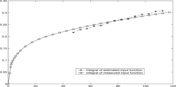
One examples of the estimated input function integral is illustrated in Fig. 1, where points 18 to 31 are used in estimation. It is noted that the estimated input function yields a consistent curve pattern, where only small variation is observed cross simulation runs. Clearly the estimated cp(t) integral matches well with the measured cp(t) integral at the late time points.
Fig. 1.

Integral version of measured input function and estimated input function in simulation, where the noise level is 25%
V. REAL DATASETS
We now examine the PET studies of healthy control subjects obtained after intravenous injection of C-11 labeled DASB, a radioligand used for imaging the serotonin transporter (SERT). Results from a typical subject are presented here. A dynamic PET study was performed with a GE Advance PET camera with an axial resolution (FWHM) of 5.8 mm, and an in plane resolution of 5.4 mm. 18 serial dynamic PET images were acquired during the first 95 minutes after injection using the following image sequence: four 15 sec, three 1 min, three 2 min, three 5 min, three 10 min, and two 20 min frames. All PET data were corrected for attenuation, injected dose and radionuclide decay. Arterial blood samples were withdrawn every 5−7 seconds during the first two minutes, then with increasing time intervals until the end of 95 minutes post injection.
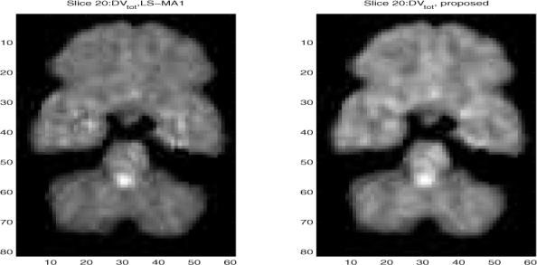
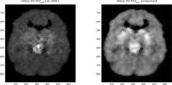
We examine the study of simultaneously estimating the input function and the parametric image by applying the proposed algorithm. As an example, we analyze single slices with number 15 and number 20 and show the VT images, where a median postfilter (with mask size is 3 × 3) was applied. For comparison with the case of measuring the input function, we report the estimated VT parametric images in Fig. 2 for Slice 15, compared with the LS-MA1 scheme; and in Fig. 3 for slice 20. The two images look similar in both cases. For example, slice 20 shows high specific binding in the basal ganglia and midbrain, consistent with high density of the serotonin transporter in these structures. We also calculated the correlation coefficient between these two DV images. It was found that the CC is as high as 0.99 and 0.97 for slice 15 and slice 20, respectively. These high CC indicates the good match between the proposed scheme and LS-MA1. However, it is worth emphasizing that the LS-MA1 algorithm requires the blood input function, therefore it serves as a performance bound.
Fig. 2.

Estimated VT parametric images after median filtering from slice number 20 of the brain PET study. (Right) when applying the proposed scheme with simultaneous estimation of the input function, and (left) when applying LS-MA1 algorithm.
Fig. 3.

Estimated VT parametric images after median filtering from slice number 20 of the brain PET study. (Left) when applying the proposed scheme with simultaneous estimation of the input function, and (right) when applying LS-MA1 algorithm.
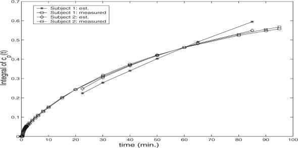
We show two examples of the estimated integral of the input function in Fig. 4. One can see that the pattern is matched to the pattern observed in the measured input function. It is worth mentioning that similar results were observed when the proposed schemes were applied to PET brain images of other control subjects.
Fig. 4.

Integral version of measured input function and estimated input function in simulation, where noise level is 25%
VI. CONCLUSION
Of interest is the estimation of parametric images describing neuroreceptor kinetics when the knowledge of the plasma input function is not available. We proposed a novel approach in estimating the input function and parametric images, by taking advantages of the specific space structure. Simulations are carried out to examine the results of the proposed scheme in estimating the input function and in revealing the underlying spatial heterogeneous structures. We also studied real brain PET data, and good performance was observed.
Acknowledgments
This work was partly supported by NSF grant No. 0000843, NIH grant No. AA11653 and NIH grant No. AG14400.
References
- 1.Ichise M, Meyer J, Yonekura Y. “An Introduction to PET and SPECT Neuroreceptor Quantification Models”. The Journal of Nuclear Medicine. 2001;42(5):755–763. [PubMed] [Google Scholar]
- 2.Gunn R, Steve R, Cunningham V. “Positron Emission Tomography Compartmental Models”. Journal of Cerebral Blood Flow and Metabolism. 2001;21(6):635–652. doi: 10.1097/00004647-200106000-00002. [DOI] [PubMed] [Google Scholar]
- 3.Chen K, Bandy D, Reiman E, Huang S, Lawson M, Feng D, Yun L, Palant A. “Noninvasive quantification of the cerebral metabolic rate for glucose using positron emission tomography, 18F-fluoro-2-deoxyglucose, the patlak method, and an image-derived input function. J. Cereb. Blood Flow Metab. 1998;18:716723. doi: 10.1097/00004647-199807000-00002. [DOI] [PubMed] [Google Scholar]
- 4.Lammertsma A, Hume S. “Simplified Reference Tissue Model for PET Receptor Studies”. Neuroimage. 1996;4(3):153–158. doi: 10.1006/nimg.1996.0066. [DOI] [PubMed] [Google Scholar]
- 5.Feng D, Wong K, Wu C, Siu W. “A Technique for Extracting Physiological Parameters and the Required Input Function Simultaneously from PET Image Measurements: Theory and Simulation Study”. IEEE Trans. Inform. Tech. Biomed. 1997 Dec.1:243–254. doi: 10.1109/4233.681168. [DOI] [PubMed] [Google Scholar]
- 6.Wong K, Meikle R, Feng D, Fulham M. “Estimation of Input Function and Kinetic Parameters Using Simulated Annealing: Application in a Flow Model”. IEEE Trans. On Nuclear Science. 2003 June;49(3) [Google Scholar]
- 7.Oikonen V. “Noise Model for PET Time-Radioactivity Curves”. Turku PET Centre Modelling Report TPCMOD0008. Jan. 19, 2003.
- 8.Logan J, Fowler J, Volkow N, Wolf A. “Graphical Analysis of Reversible Radioligand Binding from Time-Activity Measurements Applied to [N –11C – methyl]-(-)-cocaine PET Studies in Human Subjects”. J. Cereb Blood Flow Metab. 1990;10:740–747. doi: 10.1038/jcbfm.1990.127. [DOI] [PubMed] [Google Scholar]
- 9.Ichise M, Toyama H, Innis R, Carson R. “Strategies to Improve Neuroreceptor Parameter Estimation by Linear Regression Analysis”. Journal of Cerebral Blood Flow & Metabolism. 2002;22:1271–1281. doi: 10.1097/01.WCB.0000038000.34930.4E. [DOI] [PubMed] [Google Scholar]
- 10.Ichise M, Liow J. “Linearized Reference Tissue Parametric Imaging Methods: Application to [11C]DASB Positron Emission Tomography Studies of the Serotonin Transporter in Human Brain”. Journal of Cerebral Blood Flow & Metabolism. 2003;23:1096–1112. doi: 10.1097/01.WCB.0000085441.37552.CA. [DOI] [PubMed] [Google Scholar]
- 11.Talwar S, Viberg M, Paulraj A. “Blind Separation of Synchronous Co-Channel Digital Signals Using an Antenna Array - Part I: Algorithms”. IEEE Trans. on Signal Processing. 1996;44(5):1184–1197. [Google Scholar]


