Voxel based modeling and quantification of the proximal femur using inter-subject registration of quantitative CT images

Abstract

We have developed a general framework which employs quantitative computed tomography (QCT) imaging and inter-subject image registration to model the three-dimensional structure of the hip, with the goal of quantifying changes in the spatial distribution of bone as it is affected by aging, drug treatment or mechanical unloading. We have adapted rigid and non-rigid inter-subject registration techniques to transform groups of hip QCT scans into a common reference space and to construct composite proximal femoral models. We have applied this technique to a longitudinal study of 16 astronauts who on average, incurred high losses of hip bone density during spaceflights of 4–6 months on the International Space Station (ISS). We compared the pre-flight and post-flight composite hip models, and observed the gradients of the bone loss distribution. We performed paired t-tests, on a voxel by voxel basis, corrected for multiple comparisons using false discovery rate (FDR), and observed regions inside the proximal femur that showed the most significant bone loss. To validate our registration algorithm, we selected the 16 pre-flight scans and manually marked 4 landmarks for each scan. After registration, the average distance between the mapped landmarks and the corresponding landmarks in the target scan was 2.56mm. The average error due to manual landmark identification was 1.70 mm.

1. INTRODUCTION

Skeletal fracture is an epidemic problem in the elderly associated with osteoporosis, the age-related loss of bone mass and deterioration of bone structure. The most clinically important fracture site is the hip. Up to date data (4) showed that in the U.S. alone, over 2 million incident fractures at a cost of $17 billion were predicted for 2005, with hip fracture accounting for 14% of the total incident fractures, and 72% of the total cost. By 2025, annual fractures and costs are projected to rise by almost 50%. Fractures are initiated when the local tissue strength is insufficient to withstand the stress exerted by a specific loading condition at that point. Bones are three-dimensional objects that have a non-uniform distribution of strength and stiffness optimized to their respective load bearing tasks. Thus, understanding the impact of a disease process or a drug therapy on the integrity of bone depends on understanding how the disease or treatment effect is distributed throughout the bone of interest. In this study, we will develop a general framework for integrating and comparing hip QCT scans from multiple subjects. By employing inter-subject image registration, we will establish a common hip reference space to register groups of hip scans, and construct composite models in this common space for voxel based statistical comparison. As an initial exploration of this technique in a biological setting, we will apply this modeling technique in a cohort of 16 astronauts and cosmonauts with substantial proximal femoral bone loss during their 4–6 months of space missions on the International Space Station.

2. MATERIALS AND METHODS

2.1. Human subjects

We analyzed 16 pairs of pre-flight and post-flight scans from the crew of International Space Station (ISS) missions (44.6 ± 4.0 years old). Pre-flight scans were performed 30–60 days prior to launch and post-flight scans were performed within 7–10 days of landing. QCT images were acquired using a helical CT scan protocol (GE Hispeed Advantage GE Medical Systems, Milwaukee, WI) at Methodist Hospital, Baylor College of Medicine, at scanning settings of 80 kVp, 280 mAs, 3-mm slice thickness and a pitch of 1. The in-plane pixel size was 0.9375mm.

2.2. Hip inter-subject registration

Two images under registration are generally called the target (or reference) image and the source (or floating) image. In this study, we randomly selected one scan (which was from the pre-flight group) to serve as the target (reference) scan. It was visually checked to ensure the proximal femur appeared healthy and normal. All other pre-flight and post-flight scans were registered toward this reference, in other words, they were source scans during registration.

Fig. 1 illustrates using registration to compare homologous locations in different scans. In Fig. 1 (3D rendering), after scan B (source) is registered toward scan A (target), it is resampled to create a new image (C) that has the same dimensions as the target scan. To determine the grayscale value at each voxel of the resampled image, for instance (i,j,k), the transformation derived from the registration (the registration algorithm will be described later) is applied to calculate its homologous location, (x,y,z), in the original source scan. The BMD value at (x,y,z) will then be used (without alteration) as the BMD value at (i,j,k) in the resampled image (C), and it can now be compared with the BMD at (i,j,k) in the target scan (A). When (x,y,z) has non-integer values, interpolation will be applied (we used trilinear interpolation) to obtain the BMD value around that location. The resampled image (C), i.e., the registered image, looks like a “warped” image from the original scan (B). The warping refers to the fact that the transformations needed to bring the source image (B) to the registered image (C) are generally not just rigid transformations (where the total femur is considered as a rigid body, and is transformed with global translations and rotations) Rather, some local deformations must be included since the two femora are anatomically different. Our approach to derive such local deformations will be described below.

Fig. 1.

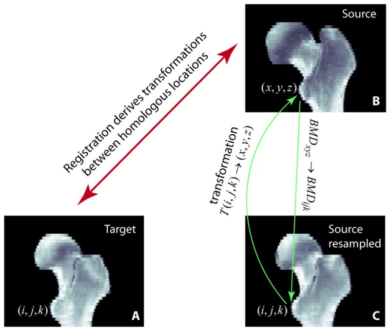
Registration establishes the geometric correspondence between homologous locations in the target (A) and the source (B). The registered image (C) is a resampled image of the source image (B). For each voxel in C, the grayscale BMD value is taken from the corresponding location in B, the original source image.

We applied a rigid registration technique that we previously developed (16) to automatically align hip QCT scans. The rigid transformations include 3 translations and 3 rotations. The algorithm is based on normalized mutual information (18), with simplex optimization under a multi-resolution scheme. It was described in more details in (16). In addition, we adapted a non-rigid registration technique originally developed for brain MRI images at Montreal Neurological Institute (6–8). It is an automatic method for volumetric image data. This non-rigid registration algorithm estimates local rigid transformations to achieve global non-rigid registration. Although locally all the transformations are rigid (translations and rotations), they are derived relatively independently (not governed by a global rigid transformation), and the resulting overall effect is non-rigid, i.e., we are able to see local deformations that we will not see if the total femur is transformed as a rigid body. The main steps are illustrated in Fig. 2. The original registration algorithm was described in details by Collins and Evans (6) and Collins et al. (7).

Fig. 2.

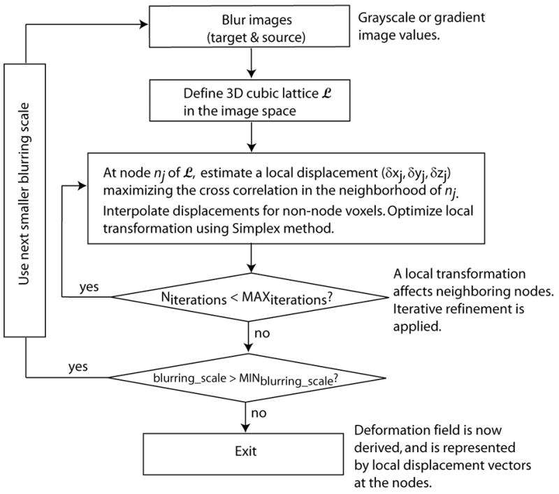
Diagram of the main steps of the non-rigid registration.

Since the scans had different spatial resolutions within the CT slices (0.9375mm) and between the slices (3mm), at the initialization step of registration, all images were first resampled to isotropic voxels, with the voxel size equal to the in-plane resolution, i.e., 0.9375mm.

2.3. Registration validation

As mentioned earlier, we selected one scan as the reference (target) scan, and all other scans were registered toward this scan. Each registered image was first visually inspected to check whether it appeared geometrically like this target image. We also quantitatively evaluated the registration errors. To do so, we manually marked landmarks in the original scans, and checked how precisely they were transformed to their homologous locations in the target image. We selected 16 scans (all the 16 pre-flight scans), and manually marked 4 anatomic landmarks in the proximal femur for each QCT scan. These landmarks were fovea capitis, trochanteric fossa, quadrate tubercle (10), and internal calcar septum (femoral “thigh spur”) (1), as illustrated in Fig. 3 (in axial view). The fovea capitis was selected as the center-most point within the fovea. The trochanteric fossa was selected as the point in the center-most portion of the concavity between the superior half of the greater trochanter and the neck, on the posterior side of the femur. The quadrate tubercle was selected as the point on the peak of the small protrusion situated on the anterior side of the femur on the inter-trochanteric line. And the internal calcar septum was selected as a point on the end of the lateral tip of the femoral “thigh spur”, where it appeared longest in an axial view.

Fig. 3.

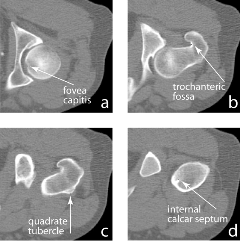
Manually identified femoral landmarks (in axial view).

After registration of each scan, the same transformation used for the image transformation was applied to the manually identified landmarks to calculate their locations in the registered image. For each of the 4 landmarks, the distance between the mapped location and its target location, where that landmark was marked in the target image, was calculated and used to evaluate the registration error.

To estimate errors due to manual landmark identification, we manually marked the four landmarks twice for each scan using two different views, and checked how they agreed with each other. One view was the original scan, and the other was the rigidly registered image. For each landmark in the original scan, after the rigid registration, we transformed it to the rigidly registered image, and compared its location against the location where the same landmark was manually marked in the rigidly registered image. Their distance was used to assess the manual landmark identification error.

2.4. Composite model construction and statistics

For each of the pre-flight and post-flight scan groups, after the scans of the 16 subjects were transformed toward the reference scan, they were superimposed, i.e., with image values from the 16 registered scans summed at each voxel, and then averaged (divided by 16) to create an average hip image. We then subtracted the pre-flight and post-flight average images to visualize the distribution of bone loss between these two groups.

Such average images alone do not reflect how bone changes vary over the 16 subjects. For example, are the observed bone changes simply dominated by any specific scan(s)? To answer such questions, we performed statistical analysis after image registration. Combining the registered images in the common reference space formed the pre-flight and post-flight composite models. Each voxel location in the composite models corresponds to 16 elements from the registered pre-flight scans, and 16 elements from the registered post-flight scans. A paired t-test can then be performed to obtain localized t-statistics. We used the conservative two-sided t-test. We performed such voxel-by-voxel t-tests through the total proximal femur, and identified voxels with statistically significant bone changes. Due to the large amount of tests performed, we used false discovery rate (FDR) (9) to provide correction for multiple comparisons. Such a correction is needed, because if we simply apply a p-value threshold for t-test results, such as 0.05, to determine which voxels are statistically significant, then 5% of the total voxels will show false positive, i.e., the numbers of voxels have the following relationship

$$N_{\mathit{false}\_\mathit{positive}}=5\%\times (N_{\mathit{true}\_\mathit{positive}}+N_{\mathit{false}\_\mathit{positive}}+N_{\mathit{true}\_\mathit{negative}}+N_{\mathit{false}\_\mathit{negative}}).$$

The ratio, N_{false _ positive}/(N_{true _ positive} + N_{false _ positive} ), can then be much higher that 5%. That is to say, if we use the criterion of p=0.05 to determine significance, among all voxels determined positive, the number of voxels that are actually false positive may be much higher than 5%. The FDR approach, on the other hand, prevents the proportion of observed significant voxels that are falsely positive from exceeding a pre-defined q-value (which we defined to be 0.05). That is, we controlled the significance level so that at most 5% of the significant voxels were false positives.

2.5. Estimation of BMD measurement errors due to mis-registration

Registration errors result in BMD measurement errors. Such errors are location specific, i.e., they depend on local registration errors as well as local BMD variations. As described earlier, we estimated the registration errors for four relatively easily identifiable landmarks (fovea capitis, trochanteric fossa, quadrate tubercle, and internal calcar septum). The registration errors at these landmarks do not necessarily represent the registration errors at other locations. To approximately estimate the BMD measurement errors due to mis-registration, we used their average registration error as the registration error of the total femur. The BMD measurement error at a specific location was estimated as the average registration error (in distance) multiplied by the BMD gradient at that location.

3. RESULTS

3.1. Hip inter-subject registration

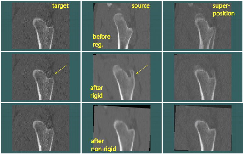
An example of the registered images is shown in Fig. 4 (in coronal view). In the top row, one slice is shown from each of two original QCT scans, i.e., the target and the source, from two different subjects (before registration). From their superimposed image on the right, we can see the body positioning difference, such as from the different shaft orientations. After registering the source scan toward the target scan using rigid registration, they were well aligned, as can be seen by comparing the superposition images in the first and the second rows. However, anatomic variability of these two hips can be seen from the two rigidly registered scans (middle row), for example, at the location pointed by the arrows. Notice that registration was only performed for the femur, not including the acetabulum, therefore the acetabular parts remained un-aligned. All subsequent calculations were confined inside the proximal femur as well. After non-rigid registration, as shown in the bottom row of Fig. 4, the source hip was warped and appeared like the target. The warping effect from rigid to non-rigid registration can be seen, for example, by comparing the transformed source images in the middle and the bottom rows at the location pointed by the arrow.

Fig. 4.

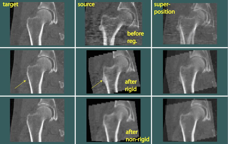
Rigid and non-rigid inter-subject registration of hip images (in coronal view). The source scan was rigidly transformed and warped toward the target scan. Arrows indicate the location where anatomical differences between the target and source can be easily seen.

An additional registration example is shown in Fig. 5 (in sagittal view). The anatomical differences between this pair of femora were rather large (such as at the location pointed by the arrows). However, the registration program still brought them to appear alike. The effects of rigid and non-rigid registration can again be seen by comparing the three superposition images on the right.

Fig. 5.

Another example of hip inter-subject registration.

3.2. Registration validation

In Table 1, validation results for the four landmarks are separately listed, and statistics for all the four landmarks are summarized (all data are summarized over 16 test scans). As shown in the top numerical row, the average distance between the homologous landmarks before registration was 9.34mm. After registration, this average distance was reduced to 2.56mm. As described in the Materials and Methods section, by identifying the landmarks in two different views, the manual landmark identification error could be assessed, which had an average value of 1.70mm.

Table 1.

Registration validation by calculating distances between landmarks in the registered images and their corresponding homologous landmarks in the target image. Manual landmark identification errors were assessed by checking how landmarks marked in two different views agreed with each other. Avg_16, Dev_16 and Max_16 are statistics (average, standard deviation and maximum) over the 16 CT scans tested.

		Distances between homologous landmarks (mm)		Manual landmark identification errors (mm)
		Before Registration	After registration
All 4 landmarks	Avg_16 Dev_16 Max_16	9.34 4.89 19.60	2.56 1.32 4.98	1.70 1.36 6.56
Fovea capitis	Avg_16 Dev_16 Max_16	12.76 4.81 19.60	2.56 1.37 4.11	1.14 1.14 3.28
Trochanteric Fossa	Avg_16 Dev_16 Max_16	8.41 4.44 19.59	2.78 1.13 4.22	1.99 1.33 3.98
Quadrate Tubercle	Avg_16 Dev_16 Max_16	7.95 4.98 17.31	2.69 1.50 4.98	1.93 1.35 5.57
Internal calcar Septum	Avg_16 Dev_16 Max_16	8.26 4.03 14.80	2.20 1.32 4.89	1.75 1.54 6.56

3.3. Composite model comparison and statistics

After scans from the pre-flight or post-flight group were registered, they were superimposed to create composite images. Fig. 6 shows a middle coronal section of the pre-flight and post-flight composite images, respectively. To include information from more voxels (for subsequent comparisons and statistics), the resampled coronal thickness here was 4.6875mm, five times of the in-plane resolution of 0.9375mm. Since the registration processes were based on the same reference scan, the two composite images appeared quite similar. However, their differences can be detected, as described below.

Fig. 6.

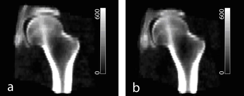
Composite images integrated from 16 subjects. (a) Pre-flight. (b) Post-flight. Grayscale values are in BMD units of mg/cm³.

Subtraction between the pre-flight and post-flight composite images shown in Fig. 6 illustrated the regional variation of bone loss through the hip (Fig. 7a). We see that regions marked by I and II showed greater magnitudes in bone loss compared to the rest. Based on voxel-by-voxel t-tests, Fig. 7b shows the derived p-value map, and Fig. 7c marks voxels that were identified as statistically significant according to FDR analysis (with q value set to be 0.05). More precisely, the average BMD of the total femur (3 dimensional) was 298.5 mg/cm³, and the average bone loss (decrease in BMD) was 24.5 mg/cm³ (−7.3%). In the coronal femur section shown in Fig. 7, the average BMD was 399.2 mg/cm³, and the average bone loss was 29.0 mg/cm³ (−8.2%). In regions I and II alone (in this coronal section), the average BMD was 333.4 mg/cm³, but the average bone loss reached 59.5 mg/cm³ (−17.8%), an over two-fold difference in bone changes. According to t-tests and FDR analysis based on the 16 scan pairs, as shown in Fig. 7c, regions I and II also showed statistical significance in bone changes while most of the rest regions did not.

Fig. 7.

Comparison of pre-flight and post-flight composite hip models (integrated from scans of 16 subjects). (a) shows the subtraction of the pre-flight and post-flight composite images. Regions I and II, shown as highlighted regions in the inset, experienced greater bone loss. (b) p-value map derived from t-tests of composite voxels. (c) Voxels where bone loss showing statistical significance in false discovery rate (FDR) analysis are marked white.

3.4. Estimation of BMD measurement errors due to mis-registration

Fig. 8 shows the BMD gradient map (averaged from the x, y, and z directions) of the proximate femur using the baseline composite image shown in Fig. 6a (with the proximal femur separated from the acetabulum). In regions I and II (as marked in Fig. 7a), the average BMD gradient was 10.8 (mg/cm³)/mm. Using our overestimated registration error of 2.56mm as the average registration error (which included the contributions from an average error of 1.70mm due to manual landmark identification errors), it could cause an average BMD error of 27.6 mg/cm³.

Fig. 8.

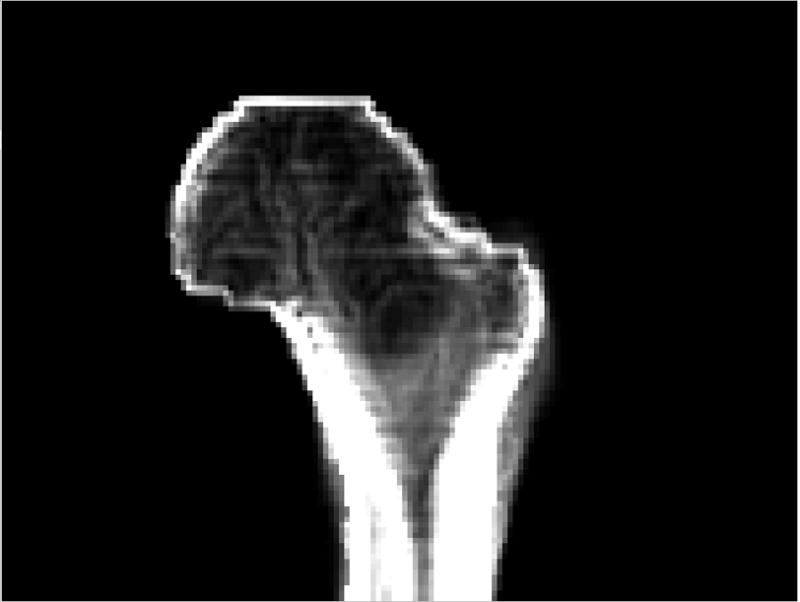
Average BMD gradient map of the proximal femur.

4. DISCUSSION

By applying inter-subject registration, we integrated hip scans into a common reference hip space. By comparing the pre-flight and post-flight composite models for 16 astronauts experiencing 4–6 months of spaceflights, we observed regions inside the femur that showed bone loss more than twice the average bone loss of the proximal femur. Focusing bone measurement on such most responsive regions can greatly improve the power of measurement. The extant paradigm of anatomic region focused DXA (dual-energy X-ray absorptiometry) and QCT measurements involves pre-selection by an experimenter of a tissue region of interest for measurements. For example, in the hip, BMD is normally reported as the average BMD of the proximal femur, or the average BMD values from the femoral neck and the trochanter (including cortical and trabecular bone) (2, 3, 15). Data from the femoral head are sometimes ignored, since it is difficult to precisely separate femoral head from the adjacent acetabulum (11). Such a paradigm essentially applies the same weighting factor to all voxels inside the anatomically defined region of interest. By using our technique to determine the spatial distribution of bone tissue response at a given skeletal site, it may be possible to better understand and interpret the effects of different bone diseases or treatment regimens. We tested our methodology using spaceflight scans, since substantial bone loss due to long-duration spaceflight has been well known. Our methodology can also be applied generically to detect changes in bone longitudinally in individuals, as well as to compare bone differences cross-sectionally. Our new measurement paradigm can be helpful in monitoring osteoporosis treatment. For example, based on current bone densitometric measurements, it generally takes one year to determine drug efficacy (before a patient knows whether he or she should switch to another drug or not), which can potentially be determined at a much shorter time if the measurement is focused at regions that are supposed to be responsive to that specific drug.

Bone from each individual can respond differently to weightlessness or other factors. Statistically identified common features can help understand how bone responds to such factors in general. An individual can compare against such common behavior (instead of comparing against other specific individuals) to estimate how this individual is deviated from the normal. For example, if the bone loss of an astronaut is determined to be serious by comparing against the composite models described here, this may suggest a need for extra exercises or countermeasures for this astronaut.

In an earlier study (14), Lang et al. reported the bone mineral density measurement for 14 of the 16 astronauts studied here. The “overall proximal femur” defined there contained the femoral neck and trochanter, but not the femoral head. Inside this region of interest (ROI), the integral bone loss was 7.95% (derived from Table 3 of Ref. (14)). Using our composite models, we also calculated (not shown) the bone loss in this ROI, which had a value of 7.90% for the 16 astronauts studied here, which agreed well with the previous study. In addition to several other much smaller sub-regions, the extensive bone loss was mainly observed in the femoral head. This could be due to focal loss in the principal compressive band of trabeculae, the medial aspect of which is located in the femoral head. The principal compressive trabecular band is one of the major load-bearing structures in the hip, and in the mechanical unloading scenario, the largest bone losses are known to occur in those regions that are most heavily loaded in normal usage.

Compared to some powerful bone modeling techniques such as finite element modeling (FEM) (5, 12, 13, 17), the voxel based modeling introduced in this paper captures more of the rich 3D information provided by QCT imaging. For example, FEM computes failure load, a parameter which is directly relevant to risk of fracture. However, besides this single parameter, much of the information on 3D distribution of material properties, stress and strain is discarded. Our framework described here provides a mechanism for potential use of such information.

The fundamental limitation of this overall approach is that registration inevitably introduces errors due to data interpolation, partial volume effect during image transformation, and errors due to mis-registration. For quantitative assessment of inter-subject registration errors, we tested how homologous landmarks could be mapped to the same location in the registered images. Our results showed that the average distance between the mapped landmarks and their target locations was 2.56mm. This is an overestimate of the registration error, since it involved contributions from an average error of 1.70mm due to manual landmark identification. In addition, when landmarks are transformed, it can shift between voxels, which would induce errors of the order of the voxel size. The registration errors obtained here are in the same order as the registration error calculated when this non-rigid registration algorithm was used for brain MRI images, which was 2.0mm (6). Due to the registration errors, this technique can not be applied to quantify thin structures such as the proximal femoral cortex. However, we are able to detect the overall bone changes at a larger scale. The two most significant bone loss regions (regions I and II in Fig. 7a) have dimensions approximately from 1cm to 2cm for both regions, which are substantially larger than the registration error. With higher image resolution and improved registration techniques, registration induced errors can be expected to be reduced.

We performed a rough estimation of the BMD measurement errors due to mis-registration. In our earlier study (16) of hip rigid registration, which involved registration error as well as BMD interpolation (partial volume effect), we calculated the BMD precision using 20 pairs of repeat scans, where the same subject was scanned twice with an interval of 15 minutes. The coefficient of variation (CV) values of the BMD measurements of the baseline and registered follow-up images, were 0.87%, 0.82%, and 1.24% for total femur integral, trabecular, and cortical BMDs (16). For inter-subject non-rigid registration, when using our overestimated registration error of 2.56mm as the average registration error (this is obviously an overestimate since it included the contributions from an average error of 1.70mm due to manual landmark identification errors), the average BMD error in regions I and II (as marked in Fig. 7a) was 27.6 mg/cm³. This would be a substantial fraction of the observed average bone loss of 59.5 mg/cm³ in these regions. However, since the directions of registration errors could be random for different subjects, it is less likely that an average bone loss of 59.5 mg/cm³ was resulted from registration errors. In addition, the registration error of 2.56mm was an overestimation can also be seen from the fact that an average registration error of 2.56mm would not be able to give the overall level of clarity of the composite image as seen in Fig. 6. Our validation method did not allow us to derive the true registration error since manual errors were involved in identifying those landmarks. Alternative registration validation methods that do not involve manual landmark identification and can derive local registration errors, such as validation based on finite element models (19), might help estimate registration errors and the induced BMD measurement errors.

In summary, by constructing composite hip models and employing voxel based statistics, we have developed a general framework for integrating and comparing groups of hip QCT images. We have demonstrated that our methods can identify the most significant bone loss regions inside the proximal femur due to spaceflight. Based on this framework, our future studies will be comparing groups of femora with experimentally measured bone strengths, and clinically recorded fracture status to identify sub-regions inside the proximal femur that are most relevant and predictive to fracture risk, and understanding how such sub-regions are affected by aging, disease and treatment.

References

- 1.Adam F, Hammer DS, Pape D, Kohn D. The internal calcar septum (femoral thigh spur) in computed tomography and conventional radiography. Skeletal Radiology. 2001;30:77–83. doi: 10.1007/s002560000308. [DOI] [PubMed] [Google Scholar]
- 2.Black DM, Bilezikian JP, Ensrud KE, Greenspan SL, Palermo L, Hue T, Lang TF, McGowan JA, Rosen CJ. One year of alendronate after one year of parathyroid hormone (1–84) for osteoporosis. N Engl J Med. 2005;353:555–65. doi: 10.1056/NEJMoa050336. [DOI] [PubMed] [Google Scholar]
- 3.Black DM, Greenspan SL, Ensrud KE, Palermo L, McGowan JA, Lang TF, Garnero P, Bouxsein ML, Bilezikian JP, Rosen CJ. The effects of parathyroid hormone and alendronate alone or in combination in postmenopausal osteoporosis. N Engl J Med. 2003;349:1207–15. doi: 10.1056/NEJMoa031975. [DOI] [PubMed] [Google Scholar]
- 4.Burge R, Dawson-Hughes B, Solomon DH, Wong JB, King A, Tosteson A. Incidence and economic burden of osteoporosis-related fractures in the United States, 2005–2025. J Bone Miner Res. 2007;22:465–75. doi: 10.1359/jbmr.061113. [DOI] [PubMed] [Google Scholar]
- 5.Cody DD, Gross GJ, Hou FJ, Spencer HJ, Goldstein SA, Fyhrie DP. Femoral strength is better predicted by finite element models than QCT and DXA. Journal of Biomechanics. 1999;32:1013–20. doi: 10.1016/s0021-9290(99)00099-8. [DOI] [PubMed] [Google Scholar]
- 6.Collins DL, Evans AC. Animal: Validation and applications of nonlinear registration-based segmentation. International Journal of Pattern Recognition and Artificial Intelligence. 1997;11:1271–1294. [Google Scholar]
- 7.Collins DL, Holmes CJ, Peters TM, Evans AC. Automatic 3-D model-based neuroanatomical segmentation. Human Brain Mapping. 1995;3:190–208. [Google Scholar]
- 8.Collins DL, Neelin P, Peters TM, Evans AC. Automatic 3D Intersubject Registration of Mr Volumetric Data in Standardized Talairach Space. Journal of Computer Assisted Tomography. 1994;18:192–205. [PubMed] [Google Scholar]
- 9.Genovese CR, Lazar NA, Nichols T. Thresholding of statistical maps in functional neuroimaging using the false discovery rate. Neuroimage. 2002;15:870–878. doi: 10.1006/nimg.2001.1037. [DOI] [PubMed] [Google Scholar]
- 10.Gray H. Anatomy of the human body. Philadelphia: Lea & Febiger; 1918. [Google Scholar]
- 11.Kang Y, Engelke K, Kalender WA. A new accurate and precise 3-D segmentation method for skeletal structures in volumetric CT data. Ieee Transactions on Medical Imaging. 2003;22:586–598. doi: 10.1109/TMI.2003.812265. [DOI] [PubMed] [Google Scholar]
- 12.Keyak JH, Rossi SA. Estimation of femoral fracture load using finite element models: an examination of stress- and strain-based failure theories. Hamamatsu, Japan: Third Combined Meeting of the Orthopaedic Research Societies; 1998. [Google Scholar]
- 13.Keyak JH, Rossi SA. Prediction of femoral fracture load using finite element models: an examination of stress- and strain-based failure theories. Journal of Biomechanics. 2000;33:209–14. doi: 10.1016/s0021-9290(99)00152-9. [DOI] [PubMed] [Google Scholar]
- 14.Lang T, LeBlanc A, Evans H, Lu Y, Genant H, Yu A. Cortical and trabecular bone mineral loss from the spine and hip in long-duration spaceflight. J Bone Miner Res. 2004;19:1006–1012. doi: 10.1359/JBMR.040307. [DOI] [PubMed] [Google Scholar]
- 15.Lang TF, Keyak JH, Heitz MW, Augat P, Lu Y, Mathur A, Genant HK. Volumetric quantitative computed tomography of the proximal femur: precision and relation to bone strength. Bone. 1997;21:101–8. doi: 10.1016/s8756-3282(97)00072-0. [DOI] [PubMed] [Google Scholar]
- 16.Li WJ, Sode M, Saeed I, Lang T. Automated registration of hip and spine for longitudinal QCT studies: Integration with 3D densitometric and structural analysis. Bone. 2006;38:273–279. doi: 10.1016/j.bone.2005.08.014. [DOI] [PMC free article] [PubMed] [Google Scholar]
- 17.Lotz JC, Hayes WC. The use of quantitative computed tomography to estimate risk of fracture from falls. J Bone Joint Surg [Am] 1990;72:689–700. [PubMed] [Google Scholar]
- 18.Studholme C, Hill DLG, Hawkes DJ. An overlap invariant entropy measure of 3D medical image alignment. Pattern Recognition. 1999;32:71–86. [Google Scholar]
- 19.Tanner C, Schnabel JA, Degenhard A, Castellano-Smith AD, Hayes C, Leach MO, Hose DR, Hill DLG, Hawkes DJ. Validation of volume-preserving non-rigid registration: Application to contrast-enhanced MR-mammography. Lecture notes in computer science. 2002;2488:307–314. [Google Scholar]