Bootstrap Classification and Point-Based Feature Selection from Age-Staged Mouse Cerebellum Tissues of Matrix Assisted Laser Desorption/Ionization Mass Spectra using a Fuzzy Rule-Building Expert System

Abstract

A bootstrap method for point-based detection of candidate biomarker peaks has been developed from pattern classifiers. Point-based detection methods are advantageous in comparison to peak-based methods. Peak determination and selection is problematic when spectral peaks are not baseline resolved or on a varying baseline. The benefit of point-based detection is that peaks can be globally determined from the characteristic features of the entire data set (i.e., subsets of candidate points) as opposed to the traditional method of selecting peaks from individual spectra and then combining the peak list into a data set. The point-based method is demonstrated to be more effective and efficient using a synthetic data set when compared to using Mahalanobis distance for feature selection. In addition, probabilities that characterize the uniqueness of the peaks are determined.

This method was applied for detecting peaks that characterize age-specific patterns of protein expression of developing and adult mouse cerebella from matrix assisted laser desorption/ionization (MALDI) mass spectrometry (MS) data. The mice comprised three age groups; 42 adults, 19 14-day old pups, and 16 7-day old pups. Three sequential spectra were obtained from each tissue section to yield 126, 57 and 48 spectra for adult, 14-day old pup, and 7-day old pup spectra, respectively. Each spectrum comprised 71,879 mass measurements in a range of 3.5-50 kDa. A previous study revealed that 846 unique peaks were detected that were consistent for 50% of the mice in each age group¹.

A fuzzy rule-building expert system (FuRES) was applied to investigate the correlation of age with features in the MS data. FuRES detected two outlier pup-14 spectra. Prediction was evaluated using 100 bootstrap samples of 2 Latin-partitions (i.e., 50:50 split between training and prediction set) of the mice. The spectra without the outliers yielded classification rates of 99.1±0.1%, 90.1±0.8%, and 97.0±0.6% for adults, 14-day old pups, and 7-day old pups, respectively. At a 95% level of significance, 100 bootstrap samples disclosed 35 adult and 21 pup distinguishing peaks for separating adults from pups; and 8 14-day old and 15 7-day old predictive peaks for separating 14-day old pup from 7-day old pup spectra. A compressed matrix comprising 40,393 points that were outside the 95% confidence intervals of one of the two FuRES discriminants was evaluated and the classification improved significantly for all classes. When peaks that satisfied a quality criterion were integrated, the 55 integrated peak areas furnished significantly improved classification for all classes: the selected peak areas furnished classification rates of 100%, 97.3±0.6%, and 97.4±0.3% for adult, 14-day old pups, and 7-day old pups using 100 bootstrap Latin partitions evaluations with the predictions averaged. When the bootstrap size was increased to 1000 samples, the results were not significantly affected. The FuRES predictions were consistent with those obtained by discriminant partial least squares (DPLS) classifications.

Introduction

The detection of significant features in complex sets of data is an important problem. The most popular methods use feature selection to collect a peak list from each mass spectrum. These peak lists are merged into a common data set. The problem with feature selection applied to each single spectrum is that no use of mutual information among the spectra is exploited for peak integration, detection, and resolution. These three steps can be difficult when spectra contain noise, peaks are not baseline resolved, and baselines vary. The removal of noise is difficult because the MALDI peak shapes and widths vary throughout the spectrum and noise is not uniformly distributed with respect to intensity and frequency. Overlapping, split, or shoulder peaks create problems because the peak position or area may not be precisely defined. Baseline correction methods are problematic when broad peaks or peak clusters are encountered. After a peak list is obtained, the peak binning process is subject to statistical errors with respect to the decision that two peaks in two spectra belong to the same bin or different bins. The quality of any further processing of feature-selected peaks is constrained by the ability to accurately extract the peaks from sets of spectra. Peaks that correlate with some property and furnish predictive models are then reported, and in the case of biomedical investigations, may be identified as biomarker candidates.

Point-based methods process all the points and save the difficult feature selection step to the end of the analysis. The data points will be transformed into subsets of statistically significant points that correlate with decisions made during the classification process. These characteristic subsets of points are obtained from all the spectra in the training set, therefore the influences of noise and uninformative peaks are removed. In addition, points that correspond to overlapping peaks may be split among different decisions or classification rules thereby overcoming limited resolution. Because entire sets of spectra contribute to the feature transformation using bootstrap approaches statistical significance can be measured.

Matrix assisted laser desorption/ionization (MALDI)² mass spectrometry (MS) is an important high-throughput tool for the profiling of protein and peptide distributions³. The detection of proteins directly in tissue extends the MALDI-MS experiment even further and this method is useful for imaging^4-8. The profiling of the brain proteome could be relevant to studies of the etiology and treatment of diverse disorders^{9, 10}. In this study, age related proteins are profiled by applying a fuzzy rule-building expert system¹¹ (FuRES) to MALDI-MS spectra acquired directly from tissue sections obtained from mouse cerebella.

Fuzzy rule-building expert systems provide several benefits that make them ideally suited to proteomic analyses¹². Unlike neural networks and other distributed machine learning algorithms, FuRES models are lucid in that they disclose the mechanism of inference. Because the classification model is fuzzy and soft, overlapping data can be accommodated without driving the classifier into ill-conditioned models that overfit the data. The classification tree is based on entropy minimization, so the structure of the tree reveals the inductive logic of the classifier. General rules are found at the root of the tree and precise rules are found at the leaves.

The detection of biomarkers is a difficult problem when one considers that they are confounded with biological and experimental variations. The Latin-partition method is a systematic bootstrap design to evaluate the predictability of classifiers¹³. Latin-partitions coupled with FuRES have been shown to disclose consistent peaks in MALDI-MS data that would be good candidates for trait classification¹². Having a systematic design for the bootstrapping analysis is important, because this process is used to generate the statistical measures for selecting the characteristic subsets of points from the data.

The MALDI profile tissue data were analyzed previously using traditional non-parametric univariate statistics¹. The data were grouped by age and the peak ranks based on the height of individual peaks detected from the spectra for each mouse were assigned to bins defined by peaks detected from the averaged mass spectrum¹. This method and other feature-based approaches require multiple steps such as accurate peak detection, peak integration, peak binning, and bin alignment, often with considerable manual effort on the part of the investigator.

This paper reports a facile multivariate method from which significant peaks are identified. Immediate benefits are the detection of significant shoulders and smaller peaks that would be discarded by intensity thresholds in peak detection algorithms. Another benefit is that prediction and feature detection are accomplished with one simple algorithm. These benefits are demonstrated with real and synthetic data. The synthetic data set also was evaluated using a comprehensive (i.e., all possible combinations) feature selection algorithm based on maximizing the Mahalanobis distances^{14, 15} of subsets from 1 to 6 peaks.

Theory

A reproducible ion signal (e.g., a peak) in a mass spectrum that can be used to predict some state of a biological system (e.g., a disease) is a characterizing feature. Classification methods are useful in that they construct predictive models from features in the spectra. The other key attribute of the classification model is that it is amenable to interpretation. For these cases, features in the spectra that are indicative of the biological state may be ascertained.

A classification tree is useful for complex models, because a divide and conquer approach is used to build a tree of linear classifiers. The classification process begins at the root of the tree and at each branch a decision is made regarding the inferential path until a leaf is reached which indicates the class. The path through the tree discloses the mechanism of classification. In addition, at each branch the variable loadings of the linear classifier may be studied to find characterizing variables. The inductive dichotomizer 3 (ID3) algorithm minimizes the entropy of classification to construct classification trees for which each branch is a univariate rule.¹⁶ This algorithm was extended to construct classification trees of multivariate rules for the classification of polymers by their laser desorption mass spectra.¹⁷

A fuzzy rule-building expert system (FuRES) uses fuzzy entropy of classification to build a multivariate classification tree¹¹. The incorporation of fuzzy logic helps prevent overfitting the data with the linear discriminant and accommodates overlapping and outlier data points. The fuzzy rules form more reproducible and general models than their crisp (i.e., not fuzzy) counterparts. The fuzzy trees do not partition the objects but instead all the objects and their fuzzy membership values are propagated through the tree. The minimum fuzzy membership value is obtained between a current rule at a branch in the tree and the propagating value from the root of the tree. For the temperature parameter to control the fuzziness of the logistic function the weight vectors must be normalized.

Discriminant partial least squares (DPLS) was used as a reference method. FURES has not been used extensively for this application and, we compare the results to those from DPLS for quality control. PLS is a well known method that can be used for calibration and classification¹⁸. PLS can be adapted to classification by replacing the dependent variable block (i.e., the matrix of Y values) with a binary encoded class matrix and is hence referred to as DPLS¹⁹. The DPLS models were converted to a set of linear regression coefficients using the equation below.

$$\mathbf{B}=\mathbf{W}{\left({\mathbf{P}}^{\mathrm{T}}\mathbf{W}\right)}^{-1}{\mathbf{Q}}^{\mathrm{T}}$$ (1)

for which B is the n×g matrix of regression coefficients. The number of classes is g and the number of points in the MALDI spectra is n. The matrices W, P, and Q are the PLS components all stored as columns with the number of columns corresponding to the number of latent variables. W and P have n rows and Q has g rows. In this variant of PLS, P is not normalized so there is no b term.

PLS is problematic in that the performance depends on judicious selection of the number of latent variables (i.e., components) in the model. Two criteria are used for selecting the number of latent variables so DPLS could be used as a quality control metric. The first criterion is to generate the best possible model by selecting the number of latent variables that yields the lowest root mean squared prediction error (RMSEP). Of course, this yields an optimistically biased measure of the best achievable result (i.e., lower bound on prediction error) via linear classification.

The second metric was chosen to yield the most parsimonious model from the training or calibration data set^{20, 21}. The lowest number of latent variables was selected that yielded perfect classification of the training set. The class assignment throughout this paper is made by assigning the class to the largest class estimate (i.e., output) per object. The model that was selected as the most parsimonious for perfect classification of the training estimate yielded an unbiased measure of the prediction error.

Systematic evaluation of classification performance is important to eliminate bias or coincidental results²². Typically evaluation of classifiers will use a fraction of the data as a prediction set and the remainder for the training set to eliminate bias²³. This split design approach can provide unbiased estimates of the prediction, however it is a weaker approach because different prediction results are obtained from different splits of the data into training and prediction sets.

The Latin-partition method is a bootstrapping method²⁴ that provides a systematic approach to classifier evaluation and measures of precision. It was first applied for the evaluation of a temperature constrained neural network’s ability to accurately classify mass spectra of carbamate pesticides.¹³ The method randomly partitions a set of data into training and prediction sets with several constraints. First, the data are divided by sample so that replicates from the same sample will not be contained in the prediction and training sets at the same time. Second, the proportions of the number of samples for each class are maintained between the prediction set and training set. Lastly, several training-prediction set pairs are given so that each sample is used once and only once for prediction. Because every object is used for prediction, the method makes efficient use of the data, eliminates the bias of using only a subset of well behaved prediction objects, and the results can be averaged across the bootstraps. For example, if 20% of the data were used for prediction, then 5 training-prediction sets would be generated.

Because the training-prediction sets are constructed randomly, then the method can be bootstrapped to yield precision bounds. The precision bounds characterize two sources of variation. The first is the repeatability of the training for the classifier. This source of variation is important for any classifier obtained by optimization because the model may be obtained from a local minimum or an ill-defined global optimum. The second source of variation measures the consistency between training and prediction sets of data. The dependency of the classification results with respect to the constitution of the training and prediction sets can be measured.

All evaluations were conducted in parallel, so that the compositions of the training and prediction sets were identical for different model building methods. This procedure allowed the variations among the mice and spectra to be separated. Statistically powerful tests such as the matched sample t-test and analysis of variance (ANOVA) could be used for comparing differences between and among different modes of FuRES model building and prediction. Matched sample t-tests were conducted between the squared prediction errors between pairs of treatments. ANOVA was also used and gave similar results that are not reported.

Bootstrapping Latin-partition evaluation with robust and stable classifiers such as FuRES¹¹ can be exploited to disclose points that are significantly correlated with properties or classes. The linear discriminant at each rule can be stored for every model that is built during the bootstrapping procedure. The average and standard deviation discriminants are obtained. Features of the discriminant that are not reproducible across partitions will be characterized as having large relative standard deviations. Using the t-statistic, the probability of significance can be obtained for every point in the discriminant. The t-statistic does not depend on the square root of the number of bootstrap samples.

The 95% confidence interval was used so that all points outside the threshold are deemed significant. These points were then separated into positive and negative loadings. The next step requires finding peaks in the set of significant discriminant loadings. Otherwise, some of the points may correspond to valleys between peaks or shoulders that would be difficult to identify. A simple derivative calculation is used to find peaks that have a minimum peak width. The peaks must appear in the average of the class spectra and the discriminant loadings to be selected. This step removes significant variable loadings that are not resolved from neighboring mass spectral peaks in the average spectrum because these peaks would be difficult to identify. The m/z, the maximum peak intensity of the average, the maximum peak discriminant loading, and the significance of the maximum point are stored as features.

The Mahalanobis distance^{25, 26} is a unit-less metric that measures the distance between two objects corrected for the pooled covariance. The set of peaks that generates the largest distance between classes are considered most significant. The Mahalanobis distance d between classes A and B is defined as

$$d=\sqrt{({\stackrel{‒}{X}}_A-{\stackrel{‒}{X}}_B){\mathbf{S}}^{-1}{({\stackrel{‒}{X}}_A-{\stackrel{‒}{X}}_B)}^T}$$ (2)

for which d is the distance, the class means ${\stackrel{‒}{X}}_A$ and ${\stackrel{‒}{X}}_B$ are row vectors that comprise subsets of peak areas or heights. The inverse of the pooled covariance matrix S^-1 is obtained as the within-group distributions of peak areas or heights about their corresponding class means.

All possible combinations of peaks can be evaluated using the Mahalanobis distance metric¹⁵. However, when the pool of peaks is large and the number of peaks to be selected is large the evaluation of all combinations of peaks becomes computationally intractable.

Experimental Section

The method was rigorously tested with synthetic data constructed in MATLAB 7.2 using data simulated with randomly distributed peaks and noise. The most rigorous and exemplary test will be presented here. This test contained 4 synthesized biomarker Gaussian peaks and 80 confounding Gaussian peaks with identical shapes (i.e., amplitude of 1 and width of a 50 point standard deviation). The locations of the 4 biomarkers peaks were at 2,000; 4,000; 6,000; and 8,000 points. The locations of the 80 confounding peaks were assigned using uniform random deviates. The identically shaped peaks present a much more difficult challenge to the biomarker detection algorithm because peaks could not be distinguished by shape or size, but only by position. Each confounding peak was randomly assigned to one-half of the synthetic spectra. The biomarker peaks were assigned to one-half of the synthetic spectra that constituted one of the two classes.

The data comprised 200 simulated spectra with 10,000 points and 84 peaks in class A and 80 peaks in class B. Four biomarkers peaks were unique to the 100 class A objects. Normal standard deviates were generated with means of 0 and standard deviations of 0.1 and added to every point in the data set, thus defining a signal-to-noise ratio of 10 (i.e., with respect to the Gaussian peak amplitudes of 1). Eighty confounding Gaussian peaks were generated using uniform random deviates to define their positions (i.e., average) and with the same peak widths of 50 points for the standard deviation and amplitudes of 1. Each peak was assigned randomly to one half of the synthetic spectra, so each confounding peak would be contained in a different subset of spectra.

The pure Gaussian peaks were stored to define peak integration windows, so that the peaks in the noisy spectra could be optimally integrated. However, this approach biases the evaluation in favor of the peak detection method, because the true underlying peak positions under realistic circumstances would have to be estimated from the spectra as opposed to being defined a priori.

The pure peaks were used to define peak integration windows for which the intensities were summed. The window for a peak was defined for which the peak profile was greater than the profiles of the neighboring peaks or the width was defined as four standard deviations across the bottom of the peak (i.e., 200 points). The smaller window obtained from these two criteria was used. In addition, the intensity of the underlying peak maxima were used to calculate the Mahalanobis distances. All possible combinations of peaks were evaluated by selecting subsets of 1 to 6 peaks from the 84 candidate peaks. The entire evaluation took 986 min of CPU time.

Cerebellar specimens from 77 C57Bl6 mice (Mus musculus domesticus) were analyzed. The mice comprised 42 adults (25 females and 17 males) that were 8 weeks old. The ages of the mouse pups were 14 or 7 days. There were 9 females and 10 males that were two weeks old. There were 16 one-week old mice in the study. The genders of the mice were not determined at seven days of age.

All animal procedures were performed in accordance with the Vanderbilt University Guide for Care and Use of Laboratory Animals and approved by the Institutional Animal Care and Use Committee. Mice were anesthetized by isofluorane and sacrificed by decapitation. The brains were dissected, immersed in liquid nitrogen for rapid freezing, and immediately stored at -80 °C until sectioning on a cryostat. For each mouse, each of three consecutive frozen sections (bregma -6.5 to -6.7 mm) was collected at a 14 μm thickness, deposited and dried on a gold plate, and a double spot of 0.1 μL of matrix applied under the microscope to ensure consistency of spot areas. The matrix solution was saturated in 3,5-dimethoxy-4-hydroxycinnamic acid (sinapinic acid, Sigma Chemical Co., St. Louis, MO) in acetonitrile/H₂O/trifluoroacetic acid 50:49.7:0.3.

Mass spectra were acquired by Voyager-DE™ STR MALDI mass spectrometer (Applied Biosystems, Foster City, CA). This instrument was equipped with a nitrogen laser (337 nm), and data were obtained using the linear acquisition mode under delayed extraction conditions. The laser spot size on target was approximately circular with a diameter of 25 μm. Instrument settings were an accelerating voltage of 25 kV, 91% grid voltage, 0.05% guide wire voltage, a delay time of 220 ns and a bin size of 2 ns. Three spectra (each an average of 7 acquisitions of 50 shots each) were acquired for each of the 77 mice, one on each of the three sections described above to yield 231 spectra.

Internal calibration standards were single charged alpha and beta hemoglobin chains (molecular weights [MW] of 14.982 kDa and 15.617 kDa), thymosin beta-4 and thymosin beta-10 (MWs 4.965 kDa and 4.937 kDa), cytochrome c oxidase polypeptide VIIC (MW 5.444 kDa), ubiquitin (MW 8.565 kDa), and calmodulin (MW 16.791 kDa) that have been identified in the mass spectra of C57Bl6 mice. The hemoglobin peaks had a peak width defined by a full peak width at half height of 50 points,

Each spectrum was baseline corrected by dividing the spectrum into windows that span a range of m/z 100. The minimum intensity was found in each window. An exponential function is then fit to these minima using a least squares fit. The MALDI-MS spectra were converted to ASCII text.

All data processing after the baseline correction was performed on a home-built AMD XP-M 2600+ system running at 2.5 GHz (11.5×217 MHz @ 1.875 Vcore) with 2 GB of PC3500 DDR memory on a DFI NF2 Ultra Infinity motherboard. The system operated in dual channel memory mode. The operating system was Microsoft Windows XP Pro SP2. MATLAB 7.2 with the Optimization Toolbox 3.0.2 was used to perform the calculations and generate the figures.

The 231 spectra were pared to a consistent set of 71,879 m/z measurements that spanned 3.5 to 49.8 kDa. Prior to the FuRES analysis the lossless principal component transform (PCT) was used to accelerate the training rate. Principal components were calculated only for the training data and used without modification for transforming the prediction data. The entire data analysis including the 100 bootstrap samples and 201 FuRES models in MATLAB took 170 min of computational processing time. The exact same training and prediction sets were used for comparisons among the classifiers, thus permitting matched sample comparisons and removal of variations among the individual spectra. The evaluation constructed two FuRES models for each training set. One classification tree was built from the individual spectra and the other from the average of the 3 replicate spectra for each mouse. The evaluation constructed 400 trees for 100 bootstraps of 2 Latin partitions using (231 or 229) individual and 77 average spectra.

Peaks were detected by the following procedure. The FuRES discriminant weight vectors are normalized to unit length during rule-construction. The average and standard deviation of the 200 weight vectors are calculated for the 100 bootstraps that each include 2 models. Positive and negative points in the average FuRES discriminant weight vectors were split into separate vectors that correspond to peaks, which are positively correlated with the rule. The negative peaks were multiplied by minus unity. The points were zero filled so that they would maintain correspondence with the m/z values. A double sided t-statistic was used to construct confidence intervals from the standard deviations. Data points in the average discriminant weight vector that were greater than the confidence interval were deemed significant, while the other points were set to zero. The t-statistic was not divided by the number of bootstrap samples. Peaks were detected by finding maxima that occurred within a 20 point or greater window defined by two valleys or edges (i.e., where the peak returns to baseline).

Although some shoulders and split peaks appeared to be significant, these points were discarded because ascertaining the protein or peptide identities of these features would be difficult. Several peak quality criteria were used. The maxima had to have at least 2 points on either side to be recognized as a peak. For a candidate peak window, the geometric mean of the peak class average and the weight vector had to exceed an intensity threshold of 1×10^-4. The intensity for each peak was defined as the difference between the peak maximum and the greatest intensity of its edge. The peak maxima of the class average and the discriminant had to agree within a tolerance of 10 Thomsons (i.e., m/z units²⁷).

Discussion of Results

Comparison of peak- and point-based methods using simulated data

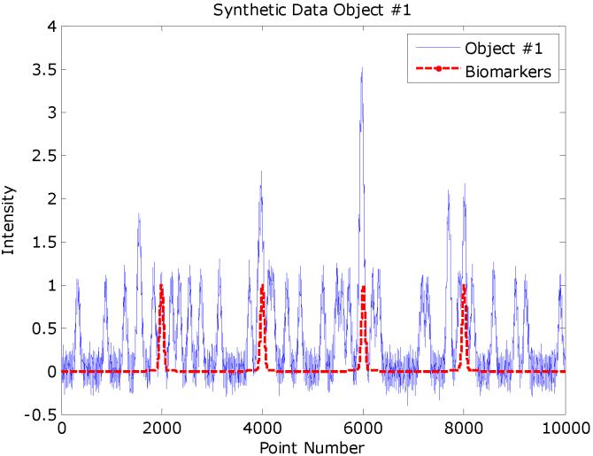
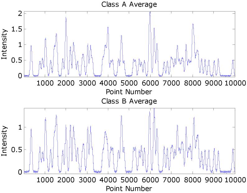
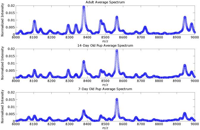
A set of simulated MALDI spectra in MATLAB were constructed that comprised 200 spectra of 10,000 data points. The signal-to-noise ratio was set to 10 using the amplitudes of the pure biomarker peaks as reference. These peaks were added to 100 of the spectra that would comprise class A, while the other 100 spectra comprise class B. Eighty confounding peaks were distributed through the spectral range. Each of these peaks was added randomly to half of the spectra (i.e., 100) in the training set. Figure 1 gives an example of a synthetic spectrum with the underlying signal. Peak amplitudes larger than unity arise from overlapping peaks. The averages synthetic spectra for each class are given in Figure 2 and note that the biomarker peaks are not obvious. Figure 3 gives the three classes averages of each class of the mice MALDI spectra for the mass range of 8,000-9,000 Th. Several peaks are overlapped and the peak widths in the synthetic data are reasonable approximations. The Hotelling T² statistic is used to define the ellipses for the scores of the first two components.

Figure 1.

Simulated spectrum with 80 randomly distributed peaks and 4 biomarker peaks. The pure signal is superimposed on the composite spectrum.

Figure 2.

The averages for each class of the synthetic data sets.

Figure 3.

Averages for the 3 classes of MALDI-MS spectra for a reduced range of [8, 9] kDa. The peak for ubiquitin (MW 8.565 kDa) was one of the internal mass calibration standards.

The first evaluation evaluated a conventional peak-based approach to biomarker detection using both peak heights and areas. All possible combinations of integrated peak areas were evaluated with the Mahalanobis distance. The peaks with the largest values were stored as biomarkers for comparison. Both optimal peak area and peak height were used in two separate evaluations. The results are reported for peak heights in Table 1 and for peak areas in Table 2. This procedure was biased in favor of the selection of the biomarkers. Because the pure synthetic peaks are used to define the optimal peak integration ranges, the results would be worse if the peak integration windows were ascertained directly from the simulated spectra. In reality, the peak integration windows would have to be determined from the noisy data. None of the subsets from 4 to 6 peaks found all 4 of the underlying biomarker peaks. False positives were obtained from neighboring peaks, which suggests a caveat when selecting candidate biomarker peaks using peak-based methods. Peaks that are not baseline resolved from the biomarker peak may appear to be correlated with the class definition, but it is in reality the neighboring biomarker peak that is affecting the correlation.

Table 1.

Peaks that give the maximum Mahalanobis distance (MD) for all possible combinations of peaks heights.

Number of Biomarkers	Number of Combinations	MD	Candidate Biomarker Peak Positions
1	84	6.6	4000
2	3486	10.9	4000	6000
3	95284	17.6	5958	4000	6000
4	1929501	23.5	5977	3977	4000	6000
5	30872016	26.8	5977	3977	4000	6000	8000
6	406481544	30.3	5977	3977	4000	6000	8000	8019

Table 2.

Peaks that give the maximum Mahalanobis distance (MD) for all possible combinations of peaks areas.

Number of Biomarkers	Number of Combinations	MD	Candidate Biomarker Peak Positions
1	84	8.6	6000
2	3486	31.0	6000	5977
3	95284	106.4	6000	5958	5977
4	1929501	115.5	4000	6000	5958	5977
5	30872016	119.8	4000	6000	5958	5977	2777
6	406481544	123.5	4000	6000	8000	5958	5977	2777

One may think it is unreasonable to expect a peak-based method to perform well when the peaks are not resolved. This thought is precisely the problem with peak-based methods applied to proteomic mass spectral data. Close examination of the MALDI spectra in Figure 3 shows that many peaks are overlapping with one another and there are probably likelihood isobaric peaks in MS measurements from complex biological samples.

The point-based method uses the variable loadings of the FuRES model to find points that separate the two classes by minimizing the fuzzy entropy of classification. Peaks that are not consistently correlated with the class definitions will be averaged out by using a random boot-strap procedure. The synthetic spectra were randomly divided into two equal size sets of 100 spectra that contained 50 spectra of each class. One set is used for constructing or training the classifier while the other set is used to evaluate prediction. Then the sets are interchanged for training and prediction, so after one Latin-partition bootstrap, each spectrum is used once and only once training and prediction. This procedure was repeated 100 times to build 200 FuRES classifiers from training sets that comprised different members.

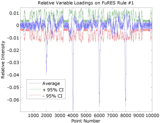
The average of the 200 FuRES variable loadings and 95% confidence intervals of each point in the classification weight were obtained and given in Figure 4. The negative peaks below the 95% confidence interval correspond to the 4 biomarker peaks in class A. Single peaks can be easily ascertained from the significant points outside the confidence interval that correspond to the underlying biomarkers. The peaks were calculated by setting windows large than the peaks and calculating sums of the points weighted by the peak intensity. The positions of the discovered biomarker peaks were 2000, 4001, 6016, and 7989. For the 100 bootstrap evaluations the average prediction rates for positive and negative classes were 95.1 ± 0.3% and 94.4 ± 0.2%.

Figure 4.

The average variable loadings from the FuRES classification tree with upper and lower 95% confidence intervals. The average was obtained from 200 averaged FuRES models acquired from 100 bootstraps of two Latin-partitions of the synthetic data. The biomarkers were located at 2,000; 4,000; 6,000; and 8,000 points.

MALDI-MS classification of mouse brain tissue samples

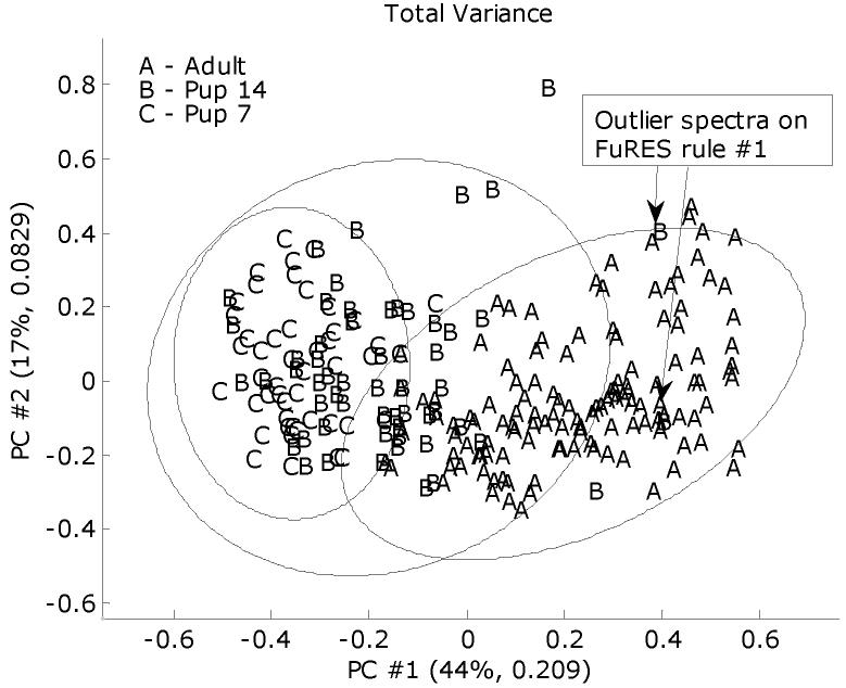
The MALDI spectra were standardized to a common mass-to-charge scale using linear interpolation that ranged between 3.5 to 49.8 kDa. The spectra were manually baseline corrected and described in the previous study¹. Each spectrum was normalized to a vector length of unity. Figure 6 gives the scores of the mean-centered spectra on the first two principal components. Note that the 14-day old group appears between the adult and 7-day old mouse spectra.

Figure 6.

PC score plot giving the overall distributions of the MALDI spectra. The 95% confidence ellipses were calculated using the Hotelling T² statistic.

Before building the FuRES tree, the spectra were transformed using principal components without mean-centering the data. The full set of object scores were used (i.e., no compression) which decreased the number of variables in the data set without losing any information. This transformation increases the speed of the FuRES calculation. The FuRES algorithm uses multivariate optimization that scales by the square of the number of variables. The principal component loadings were retained so that the FuRES weight vectors could be reconstructed in their original representation. During prediction the principal components were only calculated from the training set of data. The prediction spectra were projected onto these loadings to obtain scores.

The Latin-partition method was used for evaluation using 100 bootstrap samples of two partitions²⁸. The spectra were split into equivalent sized training and prediction sets (i.e., there were 77 mice, one set would contain 3 extra spectra). The spectra were split by mouse so at no time did the spectra from the same mouse belong to both training and prediction sets. The Latin-partitions randomly select the spectra in the training and prediction sets so that the class proportions are the same in each set. Because the partitions were equal in size, each set was used once for prediction and once for training. The prediction results are pooled for each partition and every spectrum is used once and only once for partitioning. By bootstrapping the partitioning into two training and prediction sets, two sources of variation are characterized. The first source of variation is the robustness of the FuRES model because the weight vectors are obtained from nonlinear minimizations of the fuzzy entropy. The second source of variation is the composition of the training and test set of spectra.

Table 4 gives the different classification modes for evaluating training using the Latin-partition method. The prediction results are given in confusion matrices (Tables Table 5-Table 9) that have the true classes corresponding to the rows and the FuRES predictions as columns. A perfect result would have the number of spectra in each class along the diagonals of the matrices (i.e., each confusion matrix has the number of rows and columns equal to the number of classes). Because average values for 100 bootstrap evaluations are reported, each value is also reported with its 95% confidence interval.

Table 4.

Comparison of Modes of FuRES Classification for Mouse Tissue Sections

Mode	Training	Prediction
Full	231 Individual Spectra	231 Individual Spectra
Culled	229 Individual Spectra	229 Individual Spectra
Culled	229 Individual Spectra Significant Points	299 Individual Spectra Significant Points
Culled	229 Individual Spectra Integrated Peaks	229 Individual Spectra Integrated Peaks
Culled	229 Individual Spectra	77 Average Spectra
Culled	77 Average Spectra	77 Average Spectra
Culled	229 Individual Spectra	229 Individual Spectra 77 Average Predictions
Culled	229 Individual Spectra Integrated Peaks	229 Individual Spectra 77 Average Predictions

Table 5.

Comparison of Confusion Matrices Obtained from 100×2 Latin Partitions of Individual Spectra from Full and Culled Data Sets Used for FuRES Model Building and Prediction

	Full Individual-Individual			Culled Individual-Individual
	Adult	Pup 14	Pup 7	Adult	Pup 14	Pup 7
Adult	124.6±0.2	1.4±0.2	0	124.9±0.2	1.1±0.2	0.0
Pup 14	2.8±0.2	50.1±0.4	4.2±0.4	1.3±0.1	49.5±0.5	4.2±0.4
Pup 7	0	1.5±0.3	46.5±0.3	0.0	1.4±0.3	46.6±0.3

Table 9.

Comparison of Confusion Matrices Obtained from 100×2 Latin-Partitions of Using Individual Spectra of All Data Points and Peak Areas for FuRES Model Building and Average of Predictions for Classification

	Individual-Average of Predictions			Peak Areas -Average of Predictions
	Adult	Pup 14	Pup 7	Adult	Pup 14	Pup 7
Adult	42.0	0.0	0.0	42.0	0.0	0.0
Pup 14	0.0	18.2±0.2	0.8±0.2	0.0	18.5±0.1	0.5±0.1
Pup 7	0.0	0.0	16.0	0.0	0.01±0.02	15.99±0.02

Effect of outliers

A FuRES classification tree that is obtained from the full set of spectra is given in Figure 7. The two 14-day old pup spectra that were grouped with the adult spectra after the first rule are labeled in the PC score plot in Figure 6. These two spectra were acquired on the same plate but were from different mice. There were no distinguishing features in the spectra that made them appear as outliers, other than their spectra fall out of the 95% confidence ellipses. An advantage of fuzzy systems is that they are resistant to outlier points. If these two spectra were resolved in the first rule as with other hard classification methods, the classification model could be ill-conditioned and overfit the data. When the evaluations were conducted with these outlier spectra included and excluded similar results were obtained, which is one advantage of classification trees in that they are robust with respect to outliers. The first comparison evaluated the full data set and the culled data set that had the two outlier spectra removed. In Table 5, note that inclusion of the outlier spectra did not deleteriously affect the predictions, although the results were improved with these two spectra removed. The 14-day old pup class has increased with the number of misclassification by approximately 2 which would be expected, because both outliers belonged to the 14-day old pup class. Henceforth all results were generated with these two spectra culled from the evaluation. A new tree was generated from the culled data set and is given Figure 8.

Figure 7.

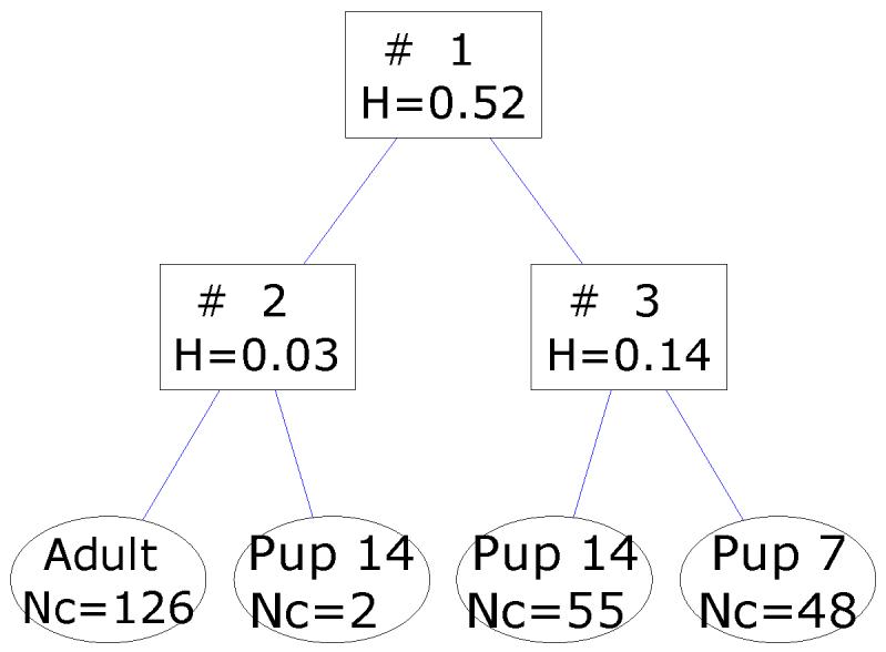
FuRES classification tree from the entire set of MALDI-MS spectra. The branches give the fuzzy entropy H. The leaves give the class identifier and number of spectra Nc.

Figure 8.

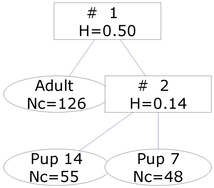
FuRES classification tree from the culled set of MALDI-MS spectra. The branches give the fuzzy entropy H. The leaves give the class identifier and number of spectra Nc.

For quality control, DPLS was used in parallel using the same input and output data as the FuRES model for each Latin partition of the individual full data set. The results are reported in Table 6 for the optimal DPLS model that yielded the lowest prediction error and the parsimonious DPLS model that yielded the model with the fewest latent variables to perfectly classify the training set. When evaluated from 1 to 100 latent variables the maximum difference between the root mean square errors of calibration between the linear and nonlinear DPLS models was 1×10^-16. The differences were attributed to rounding errors in the computation and indicate that the DPLS model is linear. All further DPLS predictions were obtained from the linearized regression coefficients²⁹.

Table 6.

Comparison of Confusion Matrices Obtained from 100×2 Latin Partitions of Individual Spectra from DPLS Optimized and DPLS Parsimonious for Individual Spectra from the Full Data Set

	Best Possible Predictions			Least LV for 100% Classification
	Adult	Pup 14	Pup 7	Adult	Pup 14	Pup 7
Adult	125.6±0.2	0.4±0.2	0	125.3±0.2	0.7±0.2	0.0
Pup 14	0.3±0.2	54.2±0.5	2.6±0.4	1.0±0.2	48.4±0.5	7.5±0.4
Pup 7	0	1.8±0.3	46.2±0.3	0.0	5.5±0.3	42.5±0.3

The FuRES confusion matrix for the full individual spectra in Table 5 is bracketed by these two validation methods. A matched sample t-test with 23099 degrees of freedom that compared the correct classifications among the 100 bootstraps of the 231 prediction objects yield a p-value of virtually zero (10^-31) that indicated FuRES predicted better than the DPLS parsimonious model and a similar result was obtained for the DPLS optimal model that predicted better than FuRES with a p-value of 10^-43. Therefore, the two control methods bracketed the FuRES prediction results, which reside between those generated by the best possible DPLS and the most parsimonious DPLS models.

Feature selection

A reduced data set was constructed by selecting the union of all the points that were outside the 95% confidence intervals of the two average discriminant weight vectors. The compression was quite modest so the full data set comprised 71,789 data points and the feature selected data points comprised 40,059 data points. However, the comparison of the confusion matrix in Table 7 with Table 5 shows an improvement for the 14-day old pups. Significant peaks were detected that satisfied the quality criteria were integrated and the peak areas were used to construct a matrix comprising 55 points and the prediction results improved further. Although some of the 95% confidence intervals may not appear to be significant, matched-sample t-tests revealed that the predictions for each class statistically improved for each feature selection step.

Table 7.

Comparison of Confusion Matrices Obtained from 100×2 Latin Partitions of Feature Selected Data Points of Individual Spectra Used for FuRES Models Building and Prediction.

	Predictions Culled Data All Points			Predictions Culled Peak Areas
	Adult	Pup 14	Pup 7	Adult	Pup 14	Pup 7
Adult	124.9±0.2	1.1±0.2	0.0	126.0	0.0	0.0
Pup 14	1.1±0.1	50.1±0.5	3.8±0.4	0.17±0.08	51.6±0.5	3.3±0.5
Pup 7	0.0	1.3±0.2	46.7±0.2	0.0	1.3±0.1	46.7±0.1

Averaging replicates versus averaging results

An interesting hypothesis that arises in classification problems is the choice of model building with a larger number of individual spectra or using averages of the replicate spectra that furnish a smaller number of higher quality spectra. In the previous study, all the replicate mass spectra from tissue sections of the same mice were averaged¹. FuRES models were built with individual spectra and average spectra from three replicates of the same mouse. The average spectra were used for the prediction set. Latin-partitions were used to construct the two confusion matrices given in Table 8. In this case, both the confusion matrices and the matched sample t-statistic revealed that models built with the individual spectra were significantly better than those built with average spectra.

Table 8.

Comparison of Confusion Matrices Obtained from 100×2 Latin-Partitions of Averaged Mouse Spectra and Individual Spectra for Model Building and Average Mouse Spectra Used for Prediction

	Culled Average-Average			Culled Individual-Average
	Adult	Pup 14	Pup 7	Adult	Pup 14	Pup 7
Adult	42.0	0.0	0.0	42.0	0.0	0.0
Pup 14	0.14±0.07	16.6±0.3	2.3±0.3	0.0	18.0±0.2	1.0±0.2
Pup 7	0.0	0.5±0.5	15.5±0.2	0.0	0.0	16.0

Alternatively, the effect of using individual spectra for prediction and then averaging the predictions for each sample was evaluated. These results are reported in Table 9 along with results obtained from the 55 peak areas and averaging the predictions. This approach did not yield improved predictions compared to training with individual spectra and predicting with the average spectra in Table 8. Differences between the average predictions and the predictions of the average spectra are indicative of nonlinearity in the classifier³⁰. Therefore, this data set appears to be linearly separable. Using the 55 peak areas and averaging the FuRES predictions significantly improved the results for the 14-day old pup class compared to using the full spectrum.

Statistically based feature selection and peak integration

The average weight vectors for each rule from the 200 FuRES models (100 bootstrap samples with 2 partitions) were calculated. This approach allows precision bounds to be obtained for the variable loadings of the discriminant weight vector as defined by the standard deviation about each weight vector average loading. All results are reported with 95% confidence intervals obtained from the t-statistic.

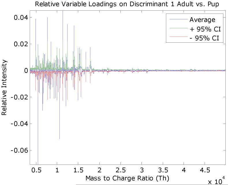
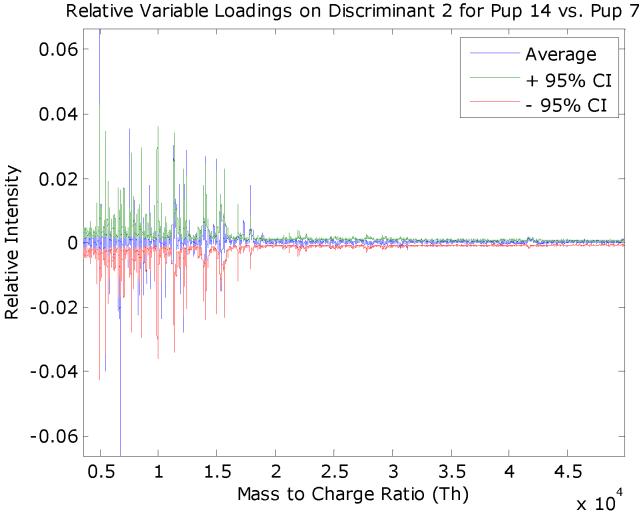
The variable loadings with 95% confidence intervals for the rule #1 discriminant, which separates the adult and pup mice spectra, is given in Figure 9. A similar plot is given in Figure 10 that separates the 7-day and 14-day mice spectra.

Figure 9.

The average FuRES discriminant vector for rule #1 that separates adult and pup spectra. The 95% confidence interval is given in red and green. Features in the weight vector that extend beyond the confidence interval are significant at a 0.05 probability. Negative features correspond to peaks that are larger in the adult spectra and positive features are those that are larger for the pup spectra.

Figure 10.

The average FuRES discriminant vector for rule #3 separates 14- and 7-day old pup spectra from 200 FuRES models. The 95% confidence interval is given in red and green. Features in the weight vector that extend beyond the confidence interval are significant at a 0.05 probability. Negative features correspond to peaks that are larger in the 14-day old pup spectra and positive features are those that are larger for the 7-day old pup spectra.

Significant points are weight vector loadings that are obtained outside the confidence interval. For each weight vector the significant points are separated by the sign of the loading into positive and negative sets. The sign of the loading corresponds to the rule and a class separation. In Figure 9, for example positive loadings are correlated with peaks that are larger for the pups and negative loadings for those correlated with the adult mice. Thus four sets of loadings (i.e., adults, pups, 14-day old pups, and 7-day old pups) were obtained from the two weight vector loadings from the two rules of the FuRES model in Figure 8. These sets of points are evaluated with several peak-quality criteria before integration into peaks to find useful candidates for identification. Some of the points may correspond to peak valleys, low intensity peaks or overlapping peaks that would be difficult to identify, so these points were removed using the following criteria to facilitate peak integration.

Peak-quality criteria were used to define candidate peaks for identification. The peaks had a minimum width of 20 Th. Consequently, the peak maximum in the average FuRES weight must have a downward slope of at least 10 Th on either side of the peak maximum. An additional intensity criterion was used so that the geometric mean of the discriminant peak maximum and the average class average exceeded 0.001. A peak list was obtained for each of the 4 sets of weights; adult, pup, 14-day pup, and 7-day pup. The four groups of mice yielded 26, 14, 7, and 8 peaks, respectively. The significance of each peak can be calculated using a t-statistic on the peak areas from the 200 discriminant loadings. The largest probability (i.e., p-value) was less than 0.001 for the discriminant peaks. Therefore, relaxing the intensity criterion would have generated a large number of discriminant peaks.

Detection and integration of peaks is facilitated because the points have been resolved into 4 sets with zeros typically separating peaks. Peaks that were not resolved were removed using the peak quality criteria. Each step, point selection and peak selection improved the predictions.

Conclusions

An automated procedure was developed for selecting biomarker peaks that uses bootstrap pattern recognition. This new point-based approach disclosed points in the spectra that offer better predictions. Because predictive points in the data are gleaned first, the peak integration is much easier because points belonging to peaks correlated to each class are resolved by the discriminant weight vector. This approach was demonstrated with FuRES models but is general and can be used with any classifier that furnishes discriminant weight vectors.

Because the points are distributed among the target properties, confounding points with no predictive power are eliminated. Thus, many of the problems of peak selection and peak binning are avoided by integrating the candidate biomarker peaks at the end of the process instead of the beginning. Furthermore, the significance of the peaks and points can be assessed by using bootstrapped Latin partitions and calculating the standard deviation about the average weight vector variable loading.

FuRES is one example of an open pattern recognition system that discloses the mechanism of inference. This capability allows the detection and study of features that may be candidates for biomarkers, in this case proteins that can lead to new discoveries and treatments for disease. FuRES provides a classification tree that can accommodate outlier spectra and the tree furnishes inductive logic regarding the structure of the spectra. The linear discriminants that are used by the FuRES rules can be interpreted as spectra. By combining FuRES with Latin-partitions, significantly relevant features can be gleaned from the data and spurious features can be removed the discriminants. FuRES is also a soft modeling method that is robust with respect to outliers in the training data sets.

Sets of statistically significant features were obtained. At a 95% level of significance, a minimum peak width of 20 amu, an intensity threshold of 0.001, and 100 bootstrap samples 26, 14, 7, and 8 predictive peaks for age were discovered for adult, pup, 14-day old pup, and 7-day old pup classes. There was an agreement of 70% for the features selected using this method compared to the features detected using nonparametric statistics¹. These features can be subjected to new experiments to elucidate the identity of the age-related mass spectral peaks.

Useful prediction results were obtained from the MALDI-MS data, especially considering that the data set was split into equal sizes for training and prediction and that the training and predictions sets comprised spectra from different mice. Usually, biological variation is a significant factor. The selected peak areas furnished classification rates of 100%, 93.7±0.6%, and 97.4±0.3% for adult, 14-day old pups, and 7-day old pups using 100 bootstrap samples using Latin partitions evaluations when the average predictions were evaluated. The significant points and integrated peaks statistically improved the prediction rates, thereby demonstrating that the selected candidate biomarker peaks have predictive power.

Building FuRES models with individual spectra as opposed to averaged spectra across replicates yields models that performed significantly better during prediction. If the classifier is robust, it can exploit the variations within the samples to yield improved models.

Figure 5.

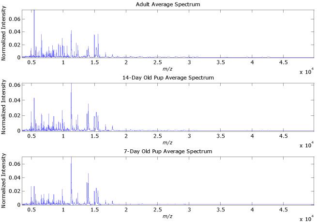
The average MALDI-MS spectra for each of the three classes of mice. The two outlier spectra have been removed.

Table 3.

Confusion Matrix of Average Predictions for 100 Bootstrap Evaluations of the Full Synthetic Data and Significant Features Defined by the 95% Confidence Interval.

	Full Data 10,000 Points		Selected 702 Points Outside the 95% Confidence Interval
	Positive	Negative	Positive	Negative
Positive	95.3±0.4	4.7±0.4	99.96±0.05	0.04±0.05
Negative	5.5±0.3	94.5±0.3	0.6±0.1	99.4±0.1

Literature Cited

- (1).Laurent C, Levinson DF, Schwartz SA, Harrington PB, Markey SP, Caprioli RM, Levitt P. Direct Profiling of the Cerebellum by MALDI MS: A Methodological Study in Postnatal and Adult Mouse. Journal of Neuroscience Research. 2005;81:613–621. doi: 10.1002/jnr.20590. [DOI] [PubMed] [Google Scholar]
- (2).Karas M, Bachmann D, Bahr U, Hillenkamp F. Matrix-Assisted Ultraviolet-Laser Desorption of Nonvolatile Compounds. International Journal of Mass Spectrometry and Ion Processes. 1987;78:53–68. [Google Scholar]
- (3).Hillenkamp F, Karas M, Beavis RC, Chait BT. Matrix-Assisted Laser Desorption Ionization Mass-Spectrometry of Biopolymers. Analytical Chemistry. 1991;63:A1193–A1202. doi: 10.1021/ac00024a002. [DOI] [PubMed] [Google Scholar]
- (4).Caprioli RM, Farmer TB, Gile J. Molecular imaging of biological samples: Localization of peptides and proteins using MALDI-TOF MS. Analytical Chemistry. 1997;69:4751–4760. doi: 10.1021/ac970888i. [DOI] [PubMed] [Google Scholar]
- (5).Caldwell RL, Caprioli RM. Tissue profiling by mass spectrometry - A review of methodology and applications. Molecular & Cellular Proteomics. 2005;4:394–401. doi: 10.1074/mcp.R500006-MCP200. [DOI] [PubMed] [Google Scholar]
- (6).Caprioli RM. Profiling and imaging of proteins in tissue sections using mass spectrometry as a discovery tool in biological research. Faseb Journal. 2004;18:C220–C220. [Google Scholar]
- (7).Chaurand P, Sanders ME, Jensen RA, Caprioli RM. Proteomics in diagnostic pathology - Profiling and imaging proteins directly in tissue sections. American Journal Of Pathology. 2004;165:1057–1068. doi: 10.1016/S0002-9440(10)63367-6. [DOI] [PMC free article] [PubMed] [Google Scholar]
- (8).Schwartz SA, Reyzer ML, Caprioli RM. Direct tissue analysis using matrix-assisted laser desorption/ionization mass spectrometry: practical aspects of sample preparation. Journal Of Mass Spectrometry. 2003;38:699–708. doi: 10.1002/jms.505. [DOI] [PubMed] [Google Scholar]
- (9).Schwartz SA, Weil RJ, Johnson MD, Toms SA, Caprioli RM. Protein profiling in brain tumors using mass spectrometry: Feasibility of a new technique for the analysis of protein expression. Clinical Cancer Research. 2004;10:981–987. doi: 10.1158/1078-0432.ccr-0927-3. [DOI] [PubMed] [Google Scholar]
- (10).Pierson J, Norris JL, Aerni HR, Svenningsson P, Caprioli RM, Andren PE. Molecular profiling of experimental Parkinson’s disease: Direct analysis of peptides and proteins on brain tissue sections by MALDI mass spectrometry. Journal Of Proteome Research. 2004;3:289–295. doi: 10.1021/pr0499747. [DOI] [PubMed] [Google Scholar]
- (11).Harrington PB. Fuzzy Multivariate Rule-Building Expert Systems - Minimal Neural Networks. Journal of Chemometrics. 1991;5:467–486. [Google Scholar]
- (12).Harrington P. d. B., Vieira NE, Chen P, Espinoza J, Nien JK, Romero R, Yergey AL. Proteomic Analysis of Amniotic Fluids Using Analysis of Variance-Principal Component Analysis and Fuzzy Rule-Building Expert Systems Applied to Matrix-Assisted Laser Desorption/Ionization Mass Spectrometry. Chemometrics and Intelligent Laboratory Systems. 2006;82:283–293. [Google Scholar]
- (13).Wan CH, Harrington PD. Screening GC-MS data for carbamate pesticides with temperature-constrained-cascade correlation neural networks. Analytica Chimica Acta. 2000;408:1–12. [Google Scholar]
- (14).Wagner M, Naik D, Pothen A. Protocols for Disease Classification from Mass Spectrometry Data. Proteomics. 2003;3:1692–1698. doi: 10.1002/pmic.200300519. [DOI] [PubMed] [Google Scholar]
- (15).Baggerly KA, Morris JS, Wang J, Gold D, Xiao LC, Coombes KR. A comprehensive approach to the analysis of matrix-assisted laser desorption/ionization-time of flight proteomics spectra from serum samples. Proteomics. 2003;3:1667–1672. doi: 10.1002/pmic.200300522. [DOI] [PubMed] [Google Scholar]
- (16).Quinlan JR. In: Machine Learning: An Artificial Intelligence Approach. Michalski RS, Carbonell JG, Mitchell TM, editors. Vol. 1. Morgan Kaufmann; Los Altos: 1983. p. 572. [Google Scholar]
- (17).Harrington PB, Voorhees KJ. Multivariate rule building expert system. Analytical Chemistry. 1990;62:729–734. [Google Scholar]
- (18).Geladi P, Kowalski BR. Partial Least-Squares Regression: A Tutorial. Analytical Chimica Acta. 1986;185:1–17. [Google Scholar]
- (19).Alsberg BK, Goodacre R, Rowland JJ, Kell DB. Classification of pyrolysis mass spectra by fuzzy multivariate rule induction-comparison with regression, K-nearest neighbour, neural and decision-tree methods. Analytica Chimica Acta. 1997;348:389–407. [Google Scholar]
- (20).Sober E. The Principle of Parsimony. British Journal for the Philosophy of Science. 1981;32:145–156. [Google Scholar]
- (21).Seasholtz MB, Kowalski B. The Parsimony Principle Applied to Multivariate Calibration. Analytica Chimica Acta. 1993;277:165–177. [Google Scholar]
- (22).Harrington PB. Statistical Validation of Classification and Calibration Models Using Bootstrapped Latin Partitions. Trends in Analytical Chemistry. 2006;25:1112–1124. [Google Scholar]
- (23).Quenouille MH. Notes on Bias Estimation. Biometrika. 1956;43:353–360. [Google Scholar]
- (24).Wehrens R, Putter H, Buydens LMC. The bootstrap: a tutorial. Chemometrics and Intelligent Laboratory Systems. 2000;64:35052. [Google Scholar]
- (25).Mahalanobis PC. On Tests and Measures of Group Divergence I. . Theoretical formulae. Journal of the Asiatic Society of Bengal. 1930;26:541–588. [Google Scholar]
- (26).Mahalanobis PC. On the Generalised Distance in Statistics. Proceedings of the National Institute of Science in India (Calcutta) 1936;A2:49–55. [Google Scholar]
- (27).Cooks RG, Rockwood AL. The ‘Thomson’. A suggested unit for mass spectroscopists. Rapid Communications in Mass Spectrometry. 1991;5:93. [Google Scholar]
- (28).Harrington PDB. Statistical validation of classification and calibration models using bootstrapped Latin partitions. Trac-Trends in Analytical Chemistry. 2006;25:1112–1124. [Google Scholar]
- (29).Martens H, Næs T. Multivariate Calibration. John Wiley; Chichester: 1989. [Google Scholar]
- (30).Harrington PD, Urbas A, Wan CH. Evaluation of neural network models with generalized sensitivity analysis. Analytical Chemistry. 2000;72:5004–5013. doi: 10.1021/ac0004963. [DOI] [PubMed] [Google Scholar]