Likelihood-mapping: A simple method to visualize phylogenetic content of a sequence alignment

Abstract

We introduce a graphical method, likelihood-mapping, to visualize the phylogenetic content of a set of aligned sequences. The method is based on an analysis of the maximum likelihoods for the three fully resolved tree topologies that can be computed for four sequences. The three likelihoods are represented as one point inside an equilateral triangle. The triangle is partitioned in different regions. One region represents star-like evolution, three regions represent a well-resolved phylogeny, and three regions reflect the situation where it is difficult to distinguish between two of the three trees. The location of the likelihoods in the triangle defines the mode of sequence evolution. If n sequences are analyzed, then the likelihoods for each subset of four sequences are mapped onto the triangle. The resulting distribution of points shows whether the data are suitable for a phylogenetic reconstruction or not.

The sequence-based study of phylogenetic relationships among different organisms has become routine. Parallel to the increasing amount of sequence information available a variety of methods have been suggested to reconstruct a phylogenetic tree (1) or a phylogenetic network (2–4). So far, few approaches have been proposed to elucidate the phylogenetic content in a set of aligned sequence a priori (5, 6). The so-called statistical geometry in sequence space analyzes the distribution of numerical invariants for all possible subsets of four sequences. The resulting distributions make it possible to distinguish between tree-, star-, and net-like geometry of the data. Moreover, based on the averages of the invariants, the method allows one to draw a graph that illustrates the mode of evolution. While the description of this diagram is straightforward if sequences consist only of purines and pyrimidines, it gets difficult if more complex alphabets (nucleic acids, amino acids) are used (7). Statistical geometry in sequence space has been successfully applied to study the evolution of tRNAs (8) or HIV (9).

In this paper, we present an alternative approach, likelihood-mapping, to display phylogenetic information contained in a sequence alignment. The method is applicable to nucleic acid sequences, amino acid sequences, or any other alphabet provided a model of sequence evolution (1, 10, 11) that can be implemented in a maximum likelihood tree reconstruction program (12, 13). Our approach allows one to visualize the tree-likeness of all quartets in a single graph and therefore renders a quick interpretation of the phylogenetic content. We will exemplify the method by applying it to simulated sequences that evolved on a star-tree or on a completely resolved tree. The analysis of two biological data sets (14, 15) will conclude the paper.

METHOD

Four Sequences.

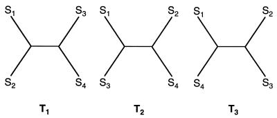
Let us consider a set of four sequences, a so-called quartet. For this quartet the maximum likelihoods (not log-likelihoods) belonging to the three possible fully resolved tree topologies (Fig. 1) are computed, using any model of sequence evolution (1, 10, 11). Let L_i be the maximum likelihood of tree T_i where i = 1, 2, 3. We can compute, according to Bayes’ theorem, the posterior probabilities

1

for each tree. Note the p_i are true probabilities satisfying p₁+ p₂ + p₃ = 1 and 0 ≤ p_i ≤ 1 in contrast to the maximum likelihoods L_i that are only conditional probabilities with L₁+ L₂+ L₃ ≠ 1. The probabilities (p₁, p₂, p₃) can be viewed as the barycentric coordinates of the point P belonging to the two-dimensional simplex

2

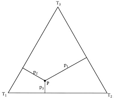
where the e_i are real valued and independent. They point to the three corners of the simplex. As a special case S₂ can be illustrated as an equilateral triangle. This construction allows an easy geometric interpretation of the p_i values. For a given point P ∈ S₂ the p_i are simply the lengths of the perpendiculars from the point P to the three sides of the triangle (Fig. 2).

Figure 1.

The fully resolved tree topologies T₁, T₂, and T₃ connecting four sequences S₁, S₂, S₃, and S₄.

Figure 2.

Map of the probability vector P = (p₁, p₂, p₃) onto an equilateral triangle. Barycentric coordinates are used, i.e. the lengths of the perpendiculars from point P to the triangle sides are equal to the probabilities p_i. The corners T₁, T₂, and T₃ represent three quartet topologies with corresponding coordinates (probabilities) (1, 0, 0), (0, 1, 0), and (0, 0, 1).

If P is close to one corner of the triangle, the likelihoods (p₁, p₂, p₃) are clearly favoring one tree over the other two. Thus, every corner of the triangle corresponds to one of the three quartet topologies T₁, T₂, or T₃. In a typical maximum-likelihood analysis one chooses the tree T_i with

3

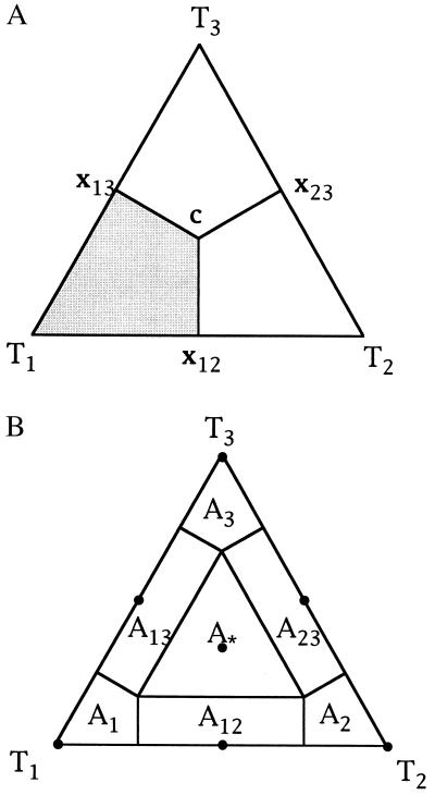
It is easy to compute the corresponding basins of attraction for each tree topology (Fig. 3A). The location of a point P in the simplex gives an immediate impression which tree is preferred.

Figure 3.

(A) Basins of attraction for the three topologies T₁, T₂, and T₃. The gray area shows the region where the probability for tree T₁ is largest. In the center c = (1/3, 1/3, 1/3) all trees are equally likely, at the points x₁₂ = (1/2, 1/2, 0), x₁₃ = (1/2, 0, 1/2), and x₂₃ = (0, 1/2, 1/2) two trees have the same likelihood whereas the remaining one has probability zero. (B) The seven basins of attraction allowing not only fully resolved trees but also the star phylogeny and three regions where it is not possible to decide between two topologies. The dots indicate the corresponding seven attractors. A₁, A₂, A₃ show the tree-like regions. A₁₂, A₁₃, A₂₃represent the net-like regions and A_∗ displays the star-like area.

Unfortunately, this picture is too optimistic. For real data it is not always possible to resolve the phylogenetic relationships of four sequences. This is either a consequence of limiting resolution due to short sequences (“noise”) or the true evolutionary tree was a star phylogeny. To account for this case, we introduce a region in the triangle S₂ representing the star phylogeny. The center c of the simplex is the point where all probabilities take on the value p_i= that is the three trees are equally likely. Thus, if P is near the center the phylogenetic relationship cannot be resolved and is better displayed by a star phylogeny. On the other hand, it also might be possible that one can exclude one of the three trees but cannot choose from among the two remaining alternatives. This is the case, if T₁ and T₂ show probabilities p₁= p₂= ½ and if p₃= 0, for example. Near point x₁₂ (see Fig. 3A) the phylogenetic relationship is best displayed by a net-like geometry that excludes tree T₃. Similarly, near points x₁₃ and x₂₃ it is impossible to unambiguously favor one tree. Based on these seven attractors in the triangle (marked with dots in Fig. 3B) the corresponding basins of attraction are easily computed. Each point in one of the seven regions has smallest Euclidean distance to its attractor. By A_∗ we denote the region where the star tree is the optimal tree. Its area equals the sum of the areas of A₁, A₂, and A₃, the regions where one tree is clearly better then the remaining ones. The regions A_ij represent the situation where we cannot distinguish trees T_i and T_j. The area of A_ij equals the sum of the area of A_i and A_j.

There is yet another way to describe the basins of attraction. If one considers the three-dimensional simplex S₃ where the fourth corner represents the star phylogeny, the basins of attraction can be viewed as projections of their corresponding volumes of the tetrahedron S₃ onto the two-dimensional plane.

The General Case.

For a set of n aligned sequences there are exactly () different possible quartets of sequences. To get an overall impression of the phylogenetic signal present in the data we compute the probability-vectors P for the quartets and draw the corresponding points in the simplex. If only few sequences are analyzed, P vectors of all () quartets are considered, otherwise a random sample of, e.g., 1,000 quartets is sufficient to obtain a comprehensive picture of the phylogenetic quality of the data set. The resulting distribution of points in the triangle S₂ forms a distinct pattern allowing us to predict a priori whether an n-taxon tree will show a good resolution or not. If most of the points P are found, e.g., in regions A₁₂, A₁₃, A₂₃, or in the star-tree region A_∗, it is clear that the overall tree will be highly multifurcating. That is, evolution was either star-like or not tree-like at all. However, the opposite conclusion is not necessarily true: Even if all quartets are completely resolved, that is, almost all P vectors are in A₁, A₂, and A₃, it is possible that the overall n-taxon tree is not completely resolved (13, 16).

Four-Cluster Likelihood-Mapping.

Instead of looking at all quartets, the analysis of tree-likeness for four disjoint groups of sequences (clusters) is also possible. Let C₁, C₂, C₃, and C₄ be a set of four clusters with c₁, c₂, c₃, and c₄ sequences. Then, we compute the probability vectors P for the c₁·c₂·c₃·c₄ possible quartets and plot the corresponding points on the triangle S₂. While the p_i values are randomly assigned to the trees T₁, T₂, and T₃, when all quartets are studied, the assignment of p_i to tree T_i is now fixed. Each tree represents one of the three possible phylogenetic relationships among the clusters. As an illustration, think of the S_i in Fig. 1 as a representative of cluster C_i. The distribution of the c₁·c₂·c₃·c₄ probability vectors over the basins of attractions allows one not only to identify the correct phylogenetic relationship of the four clusters but also shows the support for this and alternative groupings. This type of likelihood-mapping analysis is a helpful tool to illustrate how well supported an internal branch of a given tree topology is.

RESULTS

Simulation Studies.

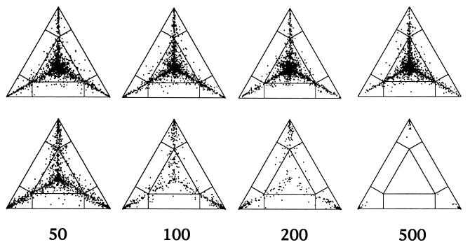
Fig. 4 displays the result of a typical likelihood-mapping analysis. A simulated set of 16 DNA-sequences was used to show the distribution of probability vectors P as a function of sequence length and the evolutionary history.

Figure 4.

Effect of sequence length (50, 100, 200, and 500 bp) on the distribution of P vectors for a simulated data set with 16 sequences. (Upper) Sequences evolving along a perfect star phylogeny. (Lower) Sequences evolving along a completely resolved tree. Sequences evolved according to the Jukes–Cantor model. The number of substitutions per site and per branch was 0.1. Each triangle shows a result of one simulation and all possible 1,820 P vectors were computed. If tree-like data were generated (Lower) the number of P vectors seems to decrease with increasing sequence length. This effect is due to the fact that identical P vectors fall on top of each other. Longer sequences increase the probability that one of the trees favored equals one. That is, most of the 1,820 P vectors superimpose each other in the corners of the triangles (cf. Table 1).

If evolution was according to a star topology then the probability vectors are concentrated in the center of the simplex with rays emanating to the corners of the triangle. This picture does not change with increasing sequence length. However, the proportion of quartets found in area A_∗ increases (Table 1). If sequence evolution followed a completely resolved tree then the proportion of points P located inside A₁+ A₂+ A₃ increases with longer sequences, as an indication that noise due to sampling artifacts is diminished. Correspondingly, the number of quartets in the remaining regions decreases. For sequences of length 500 bp the non-tree-like regions of the triangle are empty (Table 1). Thus, Fig. 4 illustrates that likelihood-mapping enables an easy distinction between star-like or tree-like evolution. The influence of sequence length (“noise”) on tree-likeness of the data is easily recognized.

Table 1.

Distribution of likelihood vectors P over the basins of attraction as a function of sequence length

Length	Star tree			Bifurcating tree
	ΣAi	A∗	ΣAij	ΣAi	A∗	ΣAij
50	17.9	77.3	4.8	61.1	32.1	6.8
100	16.2	79.6	4.2	82.0	14.3	3.7
200	11.1	85.3	3.6	91.5	5.2	3.3
500	9.8	86.5	3.7	100.0	0.0	0.0

Occupancies are shown as cumulative percentages for the three resolved regions (A₁, A₂, A₃), the star-like region (A_∗), and the three net-like regions (A₁₂, A₁₃, A₂₃). Simulation of the data assumed a start phylogeny or a perfectly bifurcating tree. 

Data Analysis.

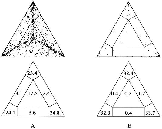
We illustrate the power of likelihood-mapping using two data sets published recently (14, 15). The first set (14) comprises eight partial cytochrome-b sequences (135 bp) and nine putative dinosaur sequences (17). The second alignment (1,850 bp) consists of ribosomal DNA from major arthropod classes (three myriapods, two chelicerates, two crustaceans, three hexapods) and six other sequences (human, Xenopus, Tubifex, Caenorhabditis, mouse, and rat). Likelihood-mapping suggests (Fig. 5) that the Zischler et al. (14) data show a fair amount of star-likeness with 17.5% of all quartet points in region A_∗ in contrast to only 0.2% for the ribosomal DNA. This result is corroborated by the bootstrap analysis as shown in refs. 14 and 15. Because of the short sequence length the percentage of quartets mapped into regions A₁₂, A₁₃, and A₂₃ is with 10.1% for the sequences from ref. 14, very high compared with 1.6% for the rDNA sequences. However, the cytochrome-b data still contain a reasonable amount of tree-likeness as 72.4% of all quartets are placed in the areas A₁, A₂,, and A₃. The tree-likeness of the ribosomal DNA is extremely high (A₁+ A₂+ A₃= 98.3%). The a posteriori analysis based on bootstrap values (15) shows that all groupings in the tree receive high support.

Figure 5.

Likelihood-mapping analysis for two biological data sets. (Upper) The distribution patterns. (Lower) The occupancies (in percent) for the seven areas of attraction. (A) Cytochrome-b data from ref. 14. (B) Ribosomal DNA of major arthropod groups (15).

Four-Cluster Likelihood Mapping.

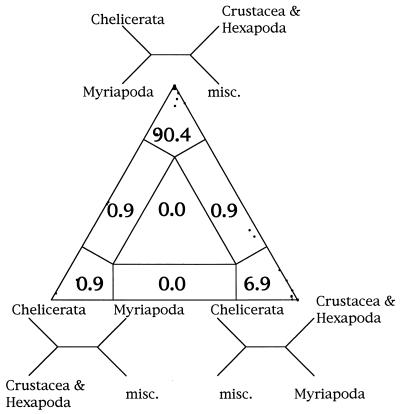
A further application of likelihood-mapping allows testing of an internal edge of a tree as given from any tree reconstruction method. As an example we consider the sister group status of myriapods and chelicerates as suggested by Friedrich and Tautz (15). Fig. 6 shows that 90.4% of all quartets between the four corresponding clusters support the branching pattern that groups chelicerates and myriapods versus crustaceans, hexapods, and the remaining sequences. We find only very low support (6.9%) for the topology that pairs myriapods with crustaceans plus hexapods rather than with chelicerates or with the rest. Based on likelihood-mapping we cannot reject the hypothesis of monophyly of myriapods and chelicerates. However, the outcome of statistical tests as suggested in ref. 18 remains to be seen. But this is outside the scope of this paper.

Figure 6.

Four-cluster likelihood-mapping of ribosomal DNA (15). Sequences were split in four disjoint groups, misc. represents the nonarthropod sequences. The corners of the triangle are labeled with the corresponding tree topologies.

DISCUSSION

The evaluation of the phylogenetic contents in a data set is of prime importance if one wants to avoid false conclusions about evolutionary relationships among organisms. Methods abound that evaluate the reliability of a reconstructed tree a posteriori (1). Likelihood-mapping† can be viewed as a complementary approach to existing methods of a priori or a posteriori evaluations of tree-likeness. Our method may be helpful when analyzing controversial phylogenies. Similar to statistical geometry in sequence space (5–7) likelihood-mapping is based on the analysis of quartets, the basic ingredients to reconstruct trees (16). Moreover, the description of seven basins of attraction (Fig. 3) that can be characterized as fully resolved (A₁, A₂, and A₃), star-like (A_∗), or intermediate between two trees (A₁₂, A₁₃, and A₂₃) is also of great importance in the quartet-puzzling tree search algorithm (13, 19). Using a variant of likelihood-mapping it is also possible to detect recombination (A.v.H., unpublished data).

Here, we have provided a simple, but versatile, approach to visualize the phylogenetic content of a data set. We have shown that the method has reasonable predictive power. While we have presented only a visual tool to analyze the phylogenetic signal of sequences it is certainly necessary to develop solid statistical tests, that provide evidence as to the significance of clusters (18) or to a deviation from tree-likeness. For example, the assumption of equal prior probability for the trees may be debatable. It remains to be seen how approaches like Jeffrey’s prior (20) or the inclusion of the variance of likelihood estimates (21) will influence the analysis.

Finally, one should keep in mind that the interpretation of the result of a likelihood-mapping analysis strongly depends on sequence length. The alignment of human mitochondrial control-region data (22) comprises 1,137 positions, and 82.5% of the quartets belong to the regions that represent fully resolved trees. Thus, the result suggests that the data are very well suited to reconstruct a well resolved tree. However, we observe 8.3% of all quartets in the star-like region A_∗ of the triangle. This value is too high for a completely resolved phylogeny (see Table 1). Therefore, we expect a phylogeny that is well resolved in certain parts of the tree only.

References

- 1.Swofford D L, Olsen G J, Waddell P J, Hillis D M. In: Molecular Systematics. Hillis D M, Moritz C, Mable B K, editors. Sunderland, MA: Sinauer; 1995. pp. 407–514. [Google Scholar]
- 2.Bandelt H-J, Dress A. Adv Math. 1992;92:47–105. [Google Scholar]
- 3.Dopazo J, Dress A, von Haeseler A. Proc Natl Acad Sci USA. 1993;90:10320–10324. doi: 10.1073/pnas.90.21.10320. [DOI] [PMC free article] [PubMed] [Google Scholar]
- 4.von Haeseler A, Churchill G A. J Mol Evol. 1993;37:77–85. doi: 10.1007/BF00170465. [DOI] [PubMed] [Google Scholar]
- 5.Eigen M, Winkler-Oswatitsch R, Dress A. Proc Natl Acad Sci USA. 1988;85:5913–5917. doi: 10.1073/pnas.85.16.5913. [DOI] [PMC free article] [PubMed] [Google Scholar]
- 6.Eigen M, Winkler-Oswatitsch R. Methods Enzymol. 1990;183:505–530. doi: 10.1016/0076-6879(90)83034-7. [DOI] [PubMed] [Google Scholar]
- 7.Nieselt-Struwe, K., Mayer, C. B. & Eigen, M. (1996) Determining the Reliability of Phylogenies with Statistical Geometry, preprint.
- 8.Eigen M, Lindemann B F, Tietze M, Winkler-Oswatitsch R, Dress A, von Haeseler A. Science. 1989;244:673–679. doi: 10.1126/science.2497522. [DOI] [PubMed] [Google Scholar]
- 9.Eigen, M. & Nieselt-Struwe, K. (1990) AIDS Suppl. 1, 4, S85–S93. [PubMed]
- 10.Zharkikh A. J Mol Evol. 1994;39:315–329. doi: 10.1007/BF00160155. [DOI] [PubMed] [Google Scholar]
- 11.Schöniger M, von Haeseler A. Mol Phylogenet Evol. 1994;3:240–247. doi: 10.1006/mpev.1994.1026. [DOI] [PubMed] [Google Scholar]
- 12.Felsenstein J. phylip version 3.5c. University of Washington, Seattle: Department of Genetics; 1993. [Google Scholar]
- 13.Strimmer K, von Haeseler A. Mol Biol Evol. 1996;13:964–969. [Google Scholar]
- 14.Zischler H, Höss M, Handt O, von Haeseler A C, van der Kuyl A, Goudsmit J, Pääbo S. Science. 1995;268:1192–1193. doi: 10.1126/science.7605504. [DOI] [PubMed] [Google Scholar]
- 15.Friedrich M, Tautz D. Nature (London) 1995;376:165–167. doi: 10.1038/376165a0. [DOI] [PubMed] [Google Scholar]
- 16.Bandelt H-J, Dress A. Adv Appl Math. 1986;7:309–343. [Google Scholar]
- 17.Woodward S R, Weynand N J, Bunnell X. Science. 1994;266:1229–1232. doi: 10.1126/science.7973705. [DOI] [PubMed] [Google Scholar]
- 18.Rzhetsky A, Kumar S, Nei M. Mol Biol Evol. 1995;12:163–167. doi: 10.1093/oxfordjournals.molbev.a040185. [DOI] [PubMed] [Google Scholar]
- 19.Strimmer K, Goldman N, von Haeseler A. Mol Biol Evol. 1997;14:210–211. [Google Scholar]
- 20.Lake J A. Proc Natl Acad Sci USA. 1995;92:9662–9666. doi: 10.1073/pnas.92.21.9662. [DOI] [PMC free article] [PubMed] [Google Scholar]
- 21.Hasegawa M, Kishino H. Evolution. 1989;43:672–677. doi: 10.1111/j.1558-5646.1989.tb04264.x. [DOI] [PubMed] [Google Scholar]
- 22.Vigilant L, Stoneking M, Harpending H, Hawkes K, Wilson A C. Science. 1991;253:1503–1507. doi: 10.1126/science.1840702. [DOI] [PubMed] [Google Scholar]