

Abstract
The dynamics by which homologous chromosomes pair is currently unknown. Here, we use fluorescence in situ hybridization in combination with three-dimensional optical microscopy to show that homologous pairing of the somatic chromosome arm 2L in Drosophila occurs by independent initiation of pairing at discrete loci rather than by a processive zippering of sites along the length of chromosome. By evaluating the pairing frequencies of 11 loci on chromosome arm 2L over several timepoints during Drosophila embryonic development, we show that all 11 loci are paired very early in Drosophila development, within 13 h after egg deposition. To elucidate whether such pairing occurs by directed or undirected motion, we analyzed the pairing kinetics of histone loci during nuclear cycle 14. By measuring changes of nuclear length and correlating these changes with progression of time during cycle 14, we were able to express the pairing frequency and distance between homologous loci as a function of time. Comparing the experimentally determined dynamics of pairing to simulations based on previously proposed models of pairing motion, we show that the observed pairing kinetics are most consistent with a constrained random walk model and not consistent with a directed motion model. Thus, we conclude that simple random contacts through diffusion could suffice to allow pairing of homologous sites.
In eukaryotes, a chromosome is sometimes aligned and associated with its homologue over part or all of its length. Although this chromosome alignment is prominent in meiosis (Roeder, 1995), for some organisms such as Dipteran insects, this association, termed homologous chromosome pairing, is observed to be a normal part of nuclear organization (Metz, 1916). Although in other organisms, less extensive homologous pairing is seen (e.g., Vourc'h et al., 1993; Lewis et al., 1993). Nevertheless, a number of intriguing biological phenomena center around homologous chromosome pairing.
Pairing of homologous chromosomes can also influence gene regulation. In Drosophila melanogaster, gene expression can be modulated by physical pairing of homologous loci in what are termed transvection and trans-sensing effects (reviewed in Tartof and Henikoff, 1991). Similar effects have been reported in such widely divergent organisms as Antirrhinum majus (Bollman et al., 1991) and Neurospora crassa (Aramayo and Metzenberg, 1996). In these cases, either suppression or enhancement of a phenotype is observed when pairing is disrupted by chromosomal rearrangements. In cases where it has been explicitly tested (e.g., Goldsborough and Kornberg, 1996), the effects can be accounted for by changes in levels of transcription that accompany the disruption of pairing. Another area where homologous pairing might play an important role is in paramutation, an interaction between alleles that leads to a directed heritable change at a locus at high frequency (Patterson and Chandler, 1995). Similarly, methylation transfer, believed to be important for many epigenetic phenomena, seems to require pairing of homologues as an initial and crucial step in the process (Colot et al., 1996).
Although progress is being made in determining the biological relevance of homologous pairing, relatively little is known about the mechanism by which homologues become paired. For both somatic and meiotic homologous pairing, this is primarily a consequence of the inability to directly monitor two homologous sites as pairing proceeds. Thus, many fundamental questions about the dynamics of how homologous chromosomes come together remain unanswered. Is the homology search carried out by discrete sites or simultaneously along the entire length of the chromosome? How do those sites that undergo homology search locate each other in the nucleus? Once homologous sites have located each other, does the pairing of adjacent sites proceed processively? Furthermore, numerous models have been put forth for how this pairing might take place (as reviewed in Loidl, 1990). In general, these models can be characterized as those emphasizing active movement of chromatin to bring homologous regions into contact or those relying mainly on fortuitous encounters of homologous sites brought about by random movements of the chromatin by diffusion (also referred to here as random walk motion). Further complicating this issue is what role, if any, does nuclear organization play in facilitating the homology search. This question has been raised by numerous meiotic studies suggesting that prealignment through bouquet formation (an alignment of telomeres and chromosomes within meiotic nuclei; reviewed in Dernburg et al., 1995; Scherthan, 1996), Rabl orientation (a centromere to telomere polarity found in interphase nuclei; Rabl, 1865; Fussell, 1987) or juxtaposition of chromosomes during metaphase congression (Maguire, 1983a ) can reduce the volume over which homology search takes place and is thus a necessary part in the meiotic pairing process. In this report, we attempt to address these questions and related ones by following the kinetics of somatic homologue pairing in Drosophila embryos.
Drosophila melanogaster offers a unique system in which to study homologous pairing. Drosophila chromosomes are thought to be homologously associated in the early stages of development in addition to their association observed during meiosis. For instance, the giant polytene chromosomes found in larval tissue exhibit a close synapsis of homologues along their entire lengths. Observations of a side-by-side juxtaposition of metaphase chromosomes in squashed neuroblast preparations lend further support that homologues pair early in development in this organism (Metz, 1916). Furthermore, examination of homologous pairing during embryogenesis of a single site has indicated that the attainment of homologous pairing for Drosophila as determined by the pairing of the histone locus occurs very early (Hiraoka et al., 1993).
There are several advantages for studying the dynamics of homologue pairing during the well-characterized stages of embryonic development (reviewed in Foe, 1993). Between the 10–13th nuclear cycles, nuclei divide in tight synchrony every 10–17 min as a monolayer at the embryo surface. At cycle 14, interphase increases in duration and is followed by a patterned mitosis where patches of cells enter mitosis at different points in time. Up until gastrulation, about an hour into cycle 14, the embryo exists as a cellular blastoderm such that cells continue to be arrayed as a monolayer at the surface of the embryo (see Fig. 1). So within one embryo, a synchronous population of nuclei in a defined orientation is available for statistical analysis of pairing events. After cycle 14, most cells, unlike at earlier stages, have defined cell fates and undergo two more cell cycles, again with patterned mitoses, ending with a terminal interphase at cycle 16. Imaginal discs and neuroblasts are the exceptions; the former undergoes one more cell division and the latter several cycles more. Although nuclei no longer behave identically at these later developmental stages, analysis of how pairing changes between the differentiated groups of cells can give us information on what factors influence a chromosome's ability to pair. Also aiding in the pairing analysis is that the embryonic developmental stages described here are all extremely amenable to the three-dimensional (3-D)1 imaging techniques needed to properly observe the pairing. Particularly useful is that many of these nuclear cycles can be imaged as they proceed in vivo, which is important for developing time courses necessary for determining the mechanisms governing the homology search.
Figure 1.

Chromosome orientation and coordinate system in cycle 13 and cycle 14 embryos. Relative orientation of the nuclei to the surface of the embryo is shown for both cycle 13 and cycle 14 embryos. Direction of Rabl orientation (centromere to telomere polarity) is also diagrammed. The bottom schematic shows the coordinate system used throughout our analysis.
To elucidate how pairing proceeds during Drosophila development, we used fluorescence in situ hybridization (FISH) and immunofluorescence under conditions that preserve nuclear and chromosomes substructure combined with high resolution 3-D optical microscopy. The pairing frequencies of 11 loci distributed over chromosome arm 2L were evaluated at several timepoints during Drosophila development. This analysis revealed that all 11 loci are paired within 13 h after egg deposition (AED), demonstrating that pairing along the entire length of the chromosome is attained very early in the Drosophila life cycle. More crucially, the frequencies of pairing at different sites indicates that side-by-side alignment is achieved through the independent initiation of pairing at discrete loci rather than by a processive zippering of sites along the length of chromosome.
We measured the time course of pairing of the histone locus through a cycle of interphase and compared our observations to computer simulations of pairing based upon different models of chromosome motion. Through quantitative kinetic analyses, we provide evidence that simple random contacts through diffusion are sufficient to allow pairing of homologous sites at the observed rates.
Materials and Methods
Drosophila Stocks
Wild-type flies were obtained from an Oregon-R stock maintained at UCSF. The lt×13 stock (Wakimoto and Hearn, 1990) was provided by B. Wakimoto (University of Washington, Seattle, WA). All stocks were maintained at 24°C.
Preparation of DNA Probes
Probes were prepared as described in Hiraoka et al. (1993) for the histone gene clone, in Dernburg et al. (1996) for the synthetic oligonucleotides (AATAG, AACAC) used to detect heterochromatic repeats, and in Marshall et al. (1996) for the P1 genomic clones. The plasmid containing the 4.8-kb HindIII fragment of Drosophila melanogaster histone genes (Lifton et al., 1977) was kindly donated by G. Karpen (Salk Institute, La Jolla, CA). The Responder (Rsp) probe was a gift from C.I. Wu (University of Chicago, IL). The P1 clones (Hartl et al., 1994) 32-95 (DS03071), 14-92 (DS01340), 16-89 (DS01529), 2-82 (DS00178), 44-63 (DS0419), 9-93 (DS00436), and 96-45 (DS09165) were obtained from the Berkeley Drosophila Genome Project. Based on salivary chromosome maps (Heino et al., 1994), the approximate distance in megabases between probes 32-94, 14-92, 16-89, 2-82, 44-63, 9-93, histone, and 96-45 are 1.8, 3.9, 4.4, 1.1, 1.1, 3.4, and 0.2 Mb. The labeling procedure, used for the histone gene clone, the oligonucleotides and the P1 clones was carried out exactly as described in Dernburg and Sedat (1997). Probe DNA (except for oligos) was first amplified using degenerate oligonucleotide-primed polymerase chain reaction. Four-base cutting restriction enzymes were then used to digest the DNA before end-labeling with either rhodamine-4-dUTP (FluoroRed; Amersham Corp., Arlington Heights, IL) or digoxigenin-dUTP (histone and oligos only) in a terminal transferase (Ratliff Biochemical, Los Alamos, NM) reaction. In some cases, fluorescein-12-dUTP (Renaissance Inc., Boston, MA) was used instead of the other fluorescent labels.
Confidence in the FISH Signal
To be confident that the observed FISH spots actually represent hybridization to the paired or unpaired location of a particular site, probes were selected or tested for unique localization. The heterochromatic sites used in this study have been previously mapped and are found mainly on chromosome 2 (Lohe et al., 1993) except for AATAG. Since AATAG satellite sequences are also found on the Y chromosome, a chromosome Y–specific probe was used to identify male embryos to exclude them from this study. The sequence AATAG was also found to a small extent on chromosome 4, however, we were able to identify the more major FISH spots corresponding to the AATAG sites on chromosome 2. To ensure that euchromatic probes made from the P1 clones also marked unique sites, neighboring clones 80 kb away were labeled with a different fluorophore and simultaneously observed with the corresponding probe to establish whether similar regions of localization could be found (data not shown). Only probes meeting this criteria were used for the subsequent pairing experiments.
Preparation of Embryos and Wing Discs
To obtain embryos in cycle 13 and early cycle 14, embryos were collected for 1 h and aged for 1.83 h before fixation. For the 4-, 6-, and 13-h timepoints, collection was set for 1 h with 3.5-, 5.5-, and 12.5-h aging periods, respectively, at 24°C. Embryos were then bleach dechorionated, fixed in 3.7% formaldehyde, and devitellinized as described by Hiraoka et al. (1993). FISH was performed using a method reported in Dernburg et al. (1996). To clearly delineate the nuclear boundaries, anti-Drosophila lamin monoclonal T40 was added and detected using either fluorescein or Cy5-conjugated goat anti–mouse secondary antibodies (Jackson ImmunoResearch Laboratories, Inc., West Grove, PA; Paddy et al. 1990). Before imaging, embryos were stained with 0.5 μg/ml DAPI in 50 mM Tris-Cl for 10 min and mounted on no. 1.5 coverslips coated with 1% poly-l-lysine to aid in embryo adherence. Most of the buffer was removed and a Vectashield antifade mounting medium (Vector Laboratories, Inc., Burlingame, CA) was applied to the embryos before sealing the coverslip to the slide with nail polish.
Wing discs were dissected from climbing third instar larvae in Robb's saline (Ashburner, 1989). The wing discs were then transferred to a hypotonic 0.7% Na citrate solution for 5–10 min and then to 45% acetic acid on a 18 × 18, no. 1.5 siliconized coverslip for 3 min. Samples were then squashed by inverting a slide over the coverslip and applying pressure. The slide was immediately transferred to 100% methanol after popping the coverslip off in liquid nitrogen. Hybridization was performed as described by Pardue (1986).
3-D, Multi-Wavelength, Fluorescence Microscopy
3-D datasets were acquired with a scientific-grade cooled CCD camera (Photometrics, Tucson, AZ) attached to an Olympus IMT-2 inverted fluorescence microscope. Action of the shutters, filter combinations, stage movement, and data collection were under the control of the Resolve3D data collection program (Chen et al., 1996) developed for use on an Indy workstation (Silicon Graphics, Sunnyvale, CA). A 60× 1.4 NA Olympus lens (0.1117 × 0.1117 pixel size in the xy-plane) and n = 1.5180 immersion oil (Cargille Laboratories, Cedar Grove, NJ) was used to image 512 × 512 pixel fields of 40–130 embryonic nuclei. Early cell cycle stages of the embryos were determined by the number of nuclei in a 512 × 512 pixel image. Each image of a 3-D stack was acquired by moving the stage in 0.5-μm intervals. For every focal position, an image was taken for each of the wavelengths corresponding to the fluorophores used in the experiment. After collection, data stacks were corrected for fluorescence bleaching and deconvolved with experimentally determined point spread functions using a constrained iterative deconvolution method (Agard et al., 1989). The wing disc squashes were collected as multiwavelength 2-D images at a single focal plane.
Analysis of Lamin and FISH Signals
The lamin signal was used to delineate the boundary of each nucleus. An outline of the lamin signal for each focal plane of the nucleus was determined by using a function that creates 2-D polygons to represent the outline. Each 2-D polygon was created semiautomatically by manually placing a seed point somewhere internal to the lamin; from this point an automatic search for the internal edge of the lamin extending radially outward from the seed point was initiated. A percentage change of intensity relative to the seed point was used to evaluate whether each encountered pixel was at the edge of the lamin signal. The actual outline pixel, selected to be at the middle of the lamin signal, was obtained by extending the location of the pixel to be a fixed distance from the determined edge. All the pixels belonging to a nucleus were obtained by grouping together all 2-D polygons with the greatest z-axis overlap. Once a set of outline points belonging to a nucleus was determined, a surface harmonic expansion was used to fit a surface to each nucleus as described in Marshall et al. (1996).
The 3-D location of each paired or unpaired FISH spot was obtained by first interactively picking a point in the vicinity of the FISH spot in each nucleus. Note that only nuclei with signals of distinct size and intensity were examined. The average signal sizes during cycle 14 for a P1 probe were 0.40 μm unpaired and 0.58 μm paired and for a histone probe were 0.54 μm unpaired and 0.62 μm paired. From that picked point, an automatic search for the maximum intensity pixel was made in an area specified by a given xy- and z-range. The 3-D location was further refined by calculating the intensity-weighted center of mass coordinates for that spot. Each FISH spot was then assigned to the nucleus whose surface enclosed it. At this point, its 3-D location was converted into the coordinate system of its assigned nucleus.
Determination of Progression in Cycle 14 Interphase from Nuclear Elongation
Embryos were bleach-dechorionated and injected at midlength as generally described in Minden (1989). 40,000 mol wt fluorescein dextran (Molecular Probes, Inc., Eugene, OR) was injected at a concentration of 2 mg/ml. Time-lapse, 3-D data stacks of embryonic nuclei starting from mid-cycle 13 interphase to mid-cycle 14 interphase were collected with our CCD-based 3-D wide-field fluorescence microscope. Using a 0.2-s exposure time, the living embryos were imaged using the same lens and oil configuration as for the hybridized embryos. The average nuclear length was obtained by measuring the top and the bottom of the nuclear volumes created by the excluded dextran. A least-squares analysis of nuclear length as a function of time determined a best-fit second degree polynomial with an R 2 value of 0.9188. Using the equation from the fit, −0.0044t 2 + 0.4371t + (4.0754 − ht) = 0 where t = time and ht = nuclear length, the time of progression for any cycle 14 embryo for the first 50 min of cycle 14 interphase was determined from knowledge of average height of the nuclei for that embryo.
Simulations
Diffusive motion was simulated using a random walk on a cubic lattice (Kao and Verkman, 1994). The average size of unpaired FISH signals was used for the size of the particles representing the unpaired loci. For each run, pairs of particles were initialized to positions reflecting the initial distribution of the site obtained from the experimentally measured average radial and vertical positions, < r o > and < z o > and their respective standard deviations, σro and σzo. A normal distribution of the particles was generated using these measured values as a starting point for the simulation. A 3-D random walk for each pair of particles was then simulated. Each iteration of the simulation represented a small time step of τ = 50 ms. At each step, the x, y, and z coordinates were incremented and decremented with equal probability by an amount δ = 2Dτ, where D is the diffusion coefficient. Spatial constraints were imposed on the entire random walk by limiting motion within a cylindrical volume specified by a radial boundary and a vertical boundary. To measure the potential range of radial and vertical positions, we measured the average radial and vertical positions < r > and < z > along with their standard deviations, σr and σz over the duration of pairing. The radial and vertical boundaries were then taken as < r > + σr and < z > ± σz. Also at each step, the pairing state and the distance between unpaired particles were calculated. Two particles were considered paired if the distance between them was less than the diameter of an particle. In these simulations, once two particles become paired, they remain paired. The results from the pairing evaluations were recorded every 20 s of the simulation. 1,000 such runs were carried out for each simulation and the results pooled to obtain the profiles of the overall pairing frequency and average inter-homologue distance as a function of time.
To simulate a directed motion model with constant velocity, the same initial conditions, boundaries, and pairing evaluations used in the random walk simulations were used. However, at each step, the positions of the two points were moved directly towards each other by an amount δ = vτ, where v is the velocity.
Results
Different Sites Along a Chromosome Arm Show Distinct Pairing Dynamics
To characterize how pairing initiates for a large chromosomal region, we hybridized probes to a series of sites spanning chromosome arm 2L at several timepoints in Drosophila development. We chose to focus on chromosome arm 2L since the pairing for one locus, the histone gene cluster, had previously been determined (Hiraoka et al., 1993) and could be compared with the pairing of other sites. FISH probes were made as described in Dernburg et al. (1996) to eight sites spanning 2L, each no more than five polytene divisions apart, and to three sites in the heterochromatin. Probes to both euchromatic and heterochromatic sites were chosen to detect any differences in pairing that might be associated with the different chromatin states. Fig. 2 A diagrams the probes and their positions along 2L.
Figure 2.

Probe positions and a typical 3-D optical data set of nuclei from a cycle 14 embryo. (A) Names and positions of probes on chromosome 2. Locations refer to cytological map positions determined by hybridization to polytene or metaphase spread chromosomes. P1 indicates that probes were derived from P1 clones. Rsp refers to the Responder locus. Probes were either labeled directly with rhodamine-4-dUTP or indirectly with digoxigenin-dUTP and detected using rhodamine, fluorescein, or Cy 5-labeled anti-digoxigenin antibodies. (B) Representative multi-wavelength 3-D data stack from a cycle 14 embryo. Each wavelength shows a subset of nine sections from a 3-D data stack of nuclei. Each section is separated by 0.5-μm focal steps starting from the top left corner and ending at the bottom right corner. FISH data from the P1 probe 09-93 (far left), and from the histone probe (middle left) together with lamin immunofluorescence (middle right) and DAPI chromatin staining (far right) were simultaneously visualized for the same set of nuclei. For most nuclei, one or two FISH signals for each probe were identified representing, respectively, the paired or unpaired states of the locus.
Embryos at several different developmental stages (2.0 [cycle 13], 2.3 [cycle 14], 4, 6, and 13 hours AED and wing discs dissected from climbing third instar larvae) were fixed and then hybridized with one or two FISH probes (see Materials and Methods). After hybridization, both embryos and wing discs were stained with antibodies to the nuclear lamin to delineate the nuclear volume. This marker was particularly useful at later stages of development when nuclei are generally smaller, more densely packed, and irregularly shaped. To confine our pairing observations to interphase nuclei, nuclei were counterstained with DAPI.
3-D images of hybridized nuclei were recorded using a wide field deconvolution optical microscope (Hiraoka et al., 1991) except in the case of the squashed wing disc preparations where 2-D images were collected. Fig. 2 B shows a representative focal series of optical sections collected from nuclei of an embryo at cycle 14. Signals corresponding to two FISH probes, the anti-lamin antibody (Fig. 2 B, middle right) and DAPI (far right) were recorded. Examination of the full 3-D nuclear volume showed that each interphase nucleus generally contained one or two FISH signals of similar size and shape that are interpreted to be the paired and unpaired homologous loci, respectively. A site was defined as paired if only one signal at twice the intensity of the unpaired locus was seen or if the 3-D distance between two signals was less than the diameter of the hybridization spot. By counting the percentage of nuclei with paired FISH signals, a pairing frequency for each of the probes was determined at different timepoints of development. The cumulative result for all the probes is shown in Fig. 3 and Table I. To visualize the spatial/temporal patterns of pairing throughout development, the pairing frequencies for the different probes for each of the selected times were plotted as a 3-D surface map.
Figure 3.

Site-specific pattern of homologous pairing for chromosome arm 2L. A surface mesh plot was fit to the measured pairing frequencies (yellow O) to better depict general trends in pairing. The height and color of the surface serve to indicate the level of pairing. High pairing frequencies are coded by increasingly darker shades of pink whereas low frequencies are represented by deepening colors of blue. Embryonic age and probe positions were spaced at equal intervals along their respective axes. Below the position axis, a probe's relative location is indicated by dashed lines to a representation of chromosome 2. Similarly, the relation between different embryonic ages is mapped to a time line drawn below the age axis.
Table I.
Pairing Frequencies for 11 Loci on Chromosome Arm 2L
| Probe | Pairing frequency | |||||||||||
|---|---|---|---|---|---|---|---|---|---|---|---|---|
| 2.0 h | 2.5 h | 4 h | 6 h | 13 h | 5 d | |||||||
| AACAC | 13 | 14 | 13 | 27 | 86 | 96 | ||||||
| Rsp | 16 | 85 | 89 | 92 | 96 | 100 | ||||||
| AATAG | 15 | 25 | 65 | 77 | 83 | 100 | ||||||
| 96-45 | 46 | 49 | 52 | 70 | 94 | 99 | ||||||
| Histone | 61 | 71 | 84 | 98 | 95 | 98 | ||||||
| 09-93 | 18 | 7 | 23 | 31 | 83 | 87 | ||||||
| 44-93 | 11 | 15 | 41 | 31 | 97 | 85 | ||||||
| 02-82 | 6 | 11 | 27 | 36 | 98 | 94 | ||||||
| 16-89 | 14 | 24 | 33 | 47 | 86 | 96 | ||||||
| 14-92 | 15 | 22 | 31 | 36 | 85 | 95 | ||||||
| 33-95 | 17 | 29 | 47 | 73 | 92 | 96 | ||||||
In all cases n > 100 nuclei.
Fig. 3 illustrates that all sites eventually pair during embryonic development but the timing of the initiation of pairing is specific to each individual locus. Between 6 and 13 h of development, all sites attain pairing levels of >60%, much greater than the low level of pairing (∼10%) seen early in development at cycle 13 for many of the sites. This increase in pairing levels continues into the larval stage (wing discs) where >95% of the nuclei contain paired loci. We note that at some time intervals, pairing at some loci appears to decrease slightly, but this is a minor effect and such sites ultimately achieve high levels of pairing. From this data it is clear that there is a significant variation in the attainment of pairing for different chromosomal sites. Of the 11 loci examined, the histone locus was observed to pair first (61% paired at cycle 13), followed by the Rsp heterochromatic locus (85% at cycle 14). By contrast, significant levels of pairing for other sites were often only seen after 6 hours of development indicating that pairing was attained considerably later for these sites.
We looked for general trends in pairing over the whole chromosome arm (Fig. 3). Previously, it has been proposed that pairing might occur through a zippering process originating at one site that would then spread processively down the chromosome arm (Lewis, 1954; Smolik-Utlaut and Gelbart, 1987; Hiraoka et al., 1993). If this were true, sites closer to the single initiation point should exhibit higher levels of pairing than those farther away, with pairing levels falling off with increasing distance from the origin. However, such a spreading phenomenon is inconsistent with our observation that during cycle 14 the histone and Rsp loci both attain higher levels of pairing than the intervening AATAG locus. Moreover, when the pairing state of two different loci are compared within the same nucleus by carrying out double-label FISH to visualize the two loci separately, we found that pairing at histone was statistically independent of pairing at 9-93 (according to a standard 2 × 2 contingency table test (Zar, 1984; P 61-65), χ2 = 0.00014, indicating that the correlation in pairing between the two sites considered is insignificant even at the 0.5 confidence level). This independent pairing of different sites on the same chromosome arm within the same nuclei is not consistent with processive spreading and rather suggests that pairing can occur at multiple independent sites along the chromosome arm.
Another possibility for the early attainment of high levels of pairing for some sites may be that repetitive loci have some preferential pairing ability because of the greater probability that a single repeat would find a matching site. Both the histone and Rsp loci, the two sites that pair the earliest, consist of several repeated sequences (Lifton et al., 1977; Lohe et al., 1993). However, examination of other repetitive probes such as the satellite sequences AATAG and AACAC, both of which show low levels of pairing at a time when both histone and Rsp show high levels of pairing, provide direct evidence that the number of repeats in a locus is not the dominant factor in the early attainment of homologous pairing.
Cells Following Different Developmental Paths Show Equivalent Pairing Levels
In later stages of embryogenesis, the initially homogeneous cell population divides into diverse cell groups, each following different developmental paths. Hence, the possibility that pairing levels could vary between each subpopulation of nuclei. We first tested whether any difference could be observed in pairing levels between nuclei destined for germline and somatic lineages. Starting at cycle 9, cells fated to form the germline (pole cells) separate from the main body of nuclei. These pole cells begin protein synthesis early and divide two more times on their own schedule. Comparison of the pairing levels from pole cell nuclei (53%, n = 19) and the main body of nuclei (60%, n = 44) for the histone locus obtained from the same cycle 14 embryo did not reveal a significant variation in pairing frequency between the two types of nuclei. In fact, the observed variation fell within the normal range found between separate internal groups of synchronized blastoderm nuclei. For instance, when four randomly chosen regions of nuclei from the same early cycle 14 embryo were examined for their levels of pairing, pairing frequencies of 39% (n = 100), 36% (n = 117), 46% (n = 118), and 40% (n = 107) were observed. This shows that a 10% range in pairing levels is within the normal fluctuation expected for measurements between synchronized populations. Similarly, no large differences were found in the pairing frequencies of the P1 09-93 locus between nuclei within the ectoderm (25%, n = 44) and mesoderm (27%, n = 26) germ layers in a 6-h AED embryo. This was particularly surprising since the size and morphology of the nuclei differed greatly between the two layers: ectoderm nuclei are columnar with an average volume of 43 μm3 whereas the mesoderm nuclei are squamous with an average volume of 69 μm3, a 60% increase in volume over the ectoderm nuclei. Therefore, at least in these cases, pairing was not affected by changes related to cell differentiation.
Pairing Does Not Require Targeting Loci to Special Regions within the Nucleus
We then wished to determine whether the position of a site in the nucleus has any influence on pairing. For example, there might be specific territories in the nucleus, such as near or on the nuclear envelope, where pairing preferentially takes place. Recently, it has been shown in Drosophila embryos that different loci reproducibly occupy different discrete regions within the nucleus (Marshall et al., 1996). Moreover, a set of loci have been identified that associate specifically with the nuclear envelope, whereas other loci are localized to a distinct internal subregion. Furthermore, theoretical considerations of how pairing could be optimized suggest that by limiting the homology search to regions adjacent to the nuclear envelope would reduce the search space from 3-D to 2-D (Loidl and Langer, 1993; Dorninger et al., 1995). If such a mechanism were operating, we would expect that sites closer to the nuclear envelope should pair more frequently than sites that are far from the nuclear periphery. Therefore, measurements were made to compare a site's distance from the nuclear envelope as well as evaluating its radial and vertical (Rabl) locations in order to look for potential differences between paired and unpaired loci (Table II). Table II shows the average radial and vertical positions of sites measured from cycle 14 embryos together with the average distance from the nuclear envelope, calculated separately for paired and unpaired sites. Using Welch's t test (Zar, 1984; P 131), the difference between the proximity of a locus to the nuclear envelope for paired and unpaired states was determined to be not significant, even at the 0.05 significance level. We then tested whether pairing is restricted to particular domains or territories within the nucleus. To explore this question, we used cycle 14 nuclei that are arranged in a monolayer on the surface of the embryo thus fixing the orientation of the nuclei so that radial and vertical distributions of a site can be measured. Based on the data from Table II, no discernible difference in spatial localization for the paired and unpaired sites for either radial or vertical positioning were found at the 0.05 significance level, using the same statistical test to compare distance from the nuclear envelope. The results did show that most sites, paired or unpaired, were contained in a confined spatial distribution imposed by the Rabl orientation as had been previously reported (Marshall et al., 1996). For each individual site, a radial confinement was also seen, but varied in extent between the different sites. Therefore, we conclude that although sites are spatially confined to a specified volume or domain in the nucleus, sites are not specially targeted to a particular nuclear territory in order to be paired.
Table II.
Comparison of Probe Position in the Nucleus for Paired and Unpaired Sites
| Radial position ± SD | Vertical position ± SD | Distance to nuclear envelope ± SD | ||||||||||||
|---|---|---|---|---|---|---|---|---|---|---|---|---|---|---|
| Probe | No. of nuclei | Paired | Unpaired | Paired | Unpaired | Paired | Unpaired | |||||||
| μm | ||||||||||||||
| AACAC | 46 | 1.38 ± 0.61 | 1.50 ± 0.48 | 3.06 ± 1.00 | 3.55 ± 0.54 | 0.62 ± 0.56 | 0.47 ± 0.59 | |||||||
| Rsp | 29 | 1.41 ± 0.83 | 1.33 ± 0.54 | 1.00 ± 0.77 | 1.36 ± 0.63 | 1.39 ± 1.02 | 1.80 ± 1.95 | |||||||
| AATAG | 61 | 0.83 ± 0.40 | 1.22 ± 0.61 | 2.96 ± 0.46 | 2.84 ± 0.92 | 0.99 ± 0.38 | 0.79 ± 0.90 | |||||||
| 96-45 | 53 | 1.06 ± 0.44 | 1.17 ± 0.51 | 3.18 ± 0.63 | 3.15 ± 0.82 | 1.42 ± 0.59 | 1.25 ± 1.45 | |||||||
| Histone | 100 | 0.95 ± 0.32 | 0.79 ± 0.34 | 0.53 ± 0.42 | 0.45 ± 0.31 | 1.60 ± 0.48 | 1.40 ± 0.48 | |||||||
| 09-93 | 38 | 1.72 ± 0.16 | 1.52 ± 0.61 | 0.18 ± 0.21 | 0.00 ± 0.65 | 0.51 ± 0.31 | 0.71 ± 1.0 | |||||||
| 44-93 | 49 | 1.12 ± 0.63 | 1.57 ± 0.53 | 0.00 ± 0.47 | 0.57 ± 0.84 | 1.30 ± 1.02 | 0.85 ± 1.10 | |||||||
| 02-82 | 41 | 2.11 ± 0.73 | 1.54 ± 0.62 | 0.24 ± 0.52 | −0.31 ± 1.15 | 0.59 ± 0.62 | 0.87 ± 1.11 | |||||||
| 16-89 | 109 | 1.57 ± 0.56 | 1.70 ± 0.59 | −1.21 ± 2.72 | −1.20 ± 2.66 | 1.01 ± 0.72 | 0.83 ± 1.08 | |||||||
| 14-92 | 85 | 1.76 ± 0.76 | 1.92 ± 0.64 | −1.53 ± 3.40 | −1.67 ± 3.54 | 0.83 ± 0.91 | 0.70 ± 1.03 | |||||||
| 32-95 | 47 | 1.20 ± 0.46 | 1.11 ± 0.54 | −1.22 ± 2.51 | −1.11 ± 2.31 | 0.28 ± 0.37 | 0.34 ± 0.64 | |||||||
Average radial positions, vertical (Rabl) positions and average distance from the nuclear envelope were measured for all the sites to determine whether any differences existed between paired and unpaired loci. Measurements were taken from cycle 14 nuclei, 7–9 μm in length. Probe order is listed from centromere proximal to distal.
Progression in Cycle 14 Interphase Determined by Changes in Nuclear Length
To analytically test models of pairing, quantitative measures of the pairing rate must be determined. However, because FISH must be carried out on fixed organisms, it is usually considered difficult to measure rates using FISH to monitor the homologous sites. Although overall developmental time courses can be determined and are very useful to study trends in pairing over large chromosomal regions, this approach does not provide a quantitative measure of the rate of pairing within a given stage. To circumvent the usual limitations preventing measurement of rates using FISH, we have developed a strategy to accurately gauge elapsed time in cycle 14 interphase by measuring changes in nuclear morphology.
The first step required exploring whether such a functional relationship actually existed for an easily and accurately measurable feature of nuclear morphology such as nuclear length. It had been previously shown by DIC microscopy that nuclear volume and diameter increase monotonically as cycle 14 interphase progresses (Foe and Alberts, 1985). In our case, changes in nuclear dimensions were tracked by injecting fluorescent dextrans into living embryos (Kalpin et al., 1994). and taking 3-D data sets of the nuclei as they progressed through the cell cycle, starting from early cycle 13 through 60 min of cycle 14 interphase (Fig. 4 A). During interphase, the high molecular weight (40,000 D) dextrans are excluded by the nuclear membrane so that nuclei image as dark holes surrounded by bright fluorescent background (Fig. 4, B and C). However, when the nuclei enter mitosis, the nuclear envelope breaks down allowing the dextran to enter where it had been previously excluded, so only an even background of fluorescence is seen (see Fig. 4 B, cyc13 t = 17.5 min). The start of a cycle is marked by the reappearance of the nuclei as dark holes (Fig. 4 B, cyc14 t = 0.0 min). When nuclear length was measured for each timepoint from the volume of each nucleus (Fig. 4 C), it was found that nuclear length increases monotonically with time in interphase of cycle 14 (Fig. 4 D). By using a least squares fit to the plotted data, a quadratic equation was found relating nuclear elongation to elapsed time in cycle 14 interphase (Fig. 4 D). This equation allows the conversion of nuclear height, which is readily measured from lamin-stained, in situ hybridized embryos into a measure of time in cycle 14 interphase providing a means by which to obtain the kinetics of pairing at that stage. Importantly, previous work using fluorescent dextrans in the live analysis of nuclear envelope breakdown and reformation in Drosophila embryos has shown that the dextrans do not disrupt the timing of the nuclear divisions (Kalpin et al., 1994).
Figure 4.

Nuclear elongation as a gauge for elapsed time in cycle 14 interphase. (A) Procedure for live analysis of nuclear volume using fluorescent-labeled dextrans. Fluorescent-labeled dextran (40,000 mol wt) is injected into the lumen of the embryo. During mitosis, dextran is able to enter into the nuclear region due to NE breakdown but at interphase, dextran is excluded from the nucleus. (B) Time series recording morphological changes in the embryonic nucleus. Single optical sections from 3-D data sets of nuclei as imaged by exclusion of the FITC-labeled dextran. Both the cell cycle stage and elapsed time in each stage is marked. Entry into mitosis is observed by the appearance of an even background of fluorescence (see cycle 13, t = 17.5 min) brought upon by the NE breakdown. The start of cycle 14 (cycle 14, t = 0.0) is set at the first reappearance of excluded nuclear volumes. (C) Representative 3-D data set of nuclei at cycle 14, t = 5.5 min showing that nuclear length can be easily determined from the excluded volume images. (D) Plot of nuclear length against elapsed time in cycle 14 interphase showing a monotonic increase in average nuclear length with increasing time. The quadratic equation was determined by a least squares fit to the plotted data where t = time and ht = nuclear ht. Such an equation allows the direct conversion from measurements of nuclear height from FISH prepared embryos into elapsed time.
Pairing of Histone Loci Occurs Early in Cycle 14
The histone locus seemed the best candidate to focus our analysis of a pairing mechanism. Besides having significantly greater levels of pairing than other loci at cycle 14, the histone locus pairs early (Fig. 3), lessening the probability that the pairing of neighboring sites would complicate the analysis through a tethering effect. From the relationship determined in Fig. 4 D and the FISH data, time profiles for the frequency of pairing as well as for temporal changes in distances between unpaired loci (inter-homologue distances) were generated to characterize pairing of the histone locus (Fig. 5). Interestingly, we found that the pairing of histone locus was relatively rapid with the majority of the pairing (80%) completed in the first 20 min of cycle 14 interphase (total duration ranges from 70–170 min, depending on the domain; Fig. 5, top). At the same time, examination of the time profile of average inter-homologue distances (Fig. 5, bottom) showed that as time increased, the average distance between unpaired loci also increased.
Figure 5.

Time profiles of histone pairing. (Top) Pairing frequency was measured from FISH signals to the histone locus in cycle 14 embryos and plotted as a function of elapsed time in interphase as measured by length of the nucleus. A substantial amount of pairing, starting from ∼20% and rising to ∼80%, is completed within the first 20 min of cycle 14 interphase. (Bottom) Average inter-homologue distance between unpaired histone loci was plotted as a function of elapsed time in interphase. The average distance between unpaired histone loci at the beginning of interphase is ∼1.2 μm apart and gradually increases to >2 μm as interphase progresses.
Distinguishing between Constrained Random Walk and Directed Models for Pairing
Having demonstrated two characteristics of how pairing developed for the histone locus in cycle 14, we next wanted to test if the observed behavior of the histone locus conforms to any of the proposed mechanisms for pairing. Two models that might account for how homologous sites become paired are either a directed motion model or random walk model for pairing (Fig. 6 A). In a simple directed motion model, homologous sites would be pulled together at some constant velocity. This type of motion could arise if inter-homologue connections were already in place to drive homologues closer together by some type of a contractile force (Holliday, 1968; Maguire, 1983a ; Smithies and Powers, 1986). Alternatively, if the homologues were already tethered together at some point, chromosome condensation could potentially bring homologous sites together (Kleckner et al., 1991). In contrast, for motion to arise from a random walk, each step taken must be independent from the previous step and random in direction (Crank, 1956). This results in the relation that the mean squared displacement in 3-D be given by the equation < r 2 > = 6Dt (Berg, 1983), where t is time and D is the diffusion coefficient that reflects how fast the random walk is occurring. Inside a nucleus, equations describing random walk motion become more complex since the confines of the nuclear volume and nonrandom distributions of the sites in the nucleus must be taken into account. For these more complicated situations, simple computer simulations can be used for describing and analyzing such motions.
Figure 6.
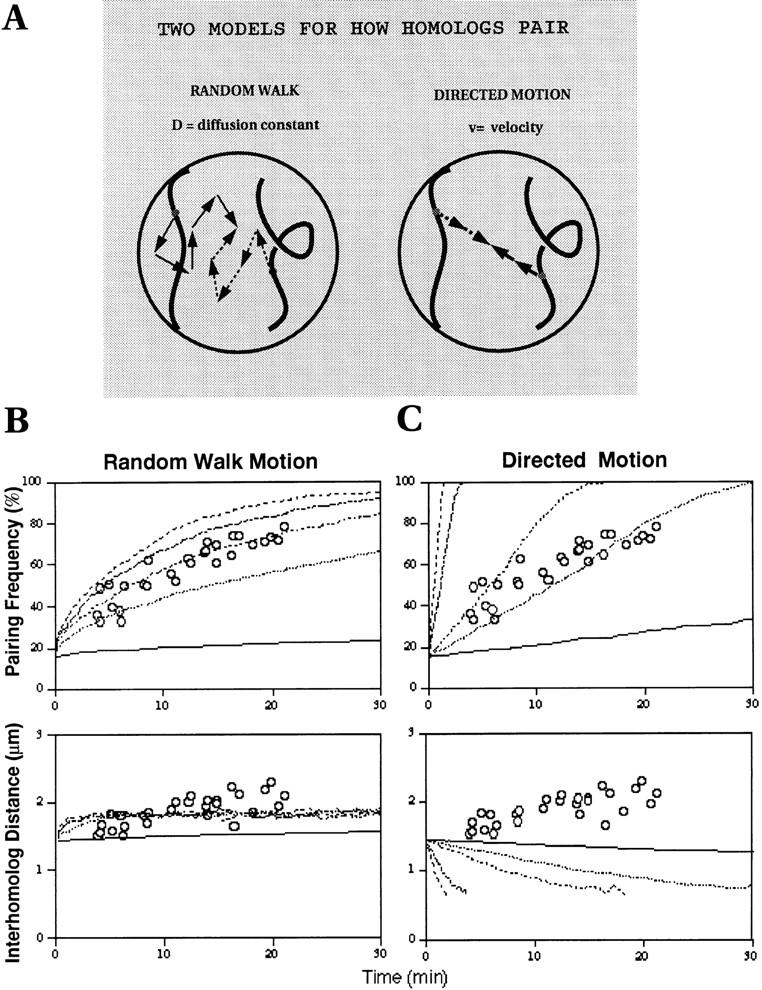
Evaluation of two potential models for homologue pairing. (A) In the random walk model, the movement of a locus can be separated into unit steps that are independent from the previous step, random in direction, and unrelated to the movements of the homologous locus. The diffusion coefficient, D, reflects how fast the random walk is occurring. In the nucleus, chromatin domains and the nuclear boundary would restrict movement from being completely random, so a constrained rather than pure random walk would be expected. In contrast, in the directed motion model, each pair of homologous loci take a unit step in a direction pointed towards the other locus. Here, a velocity constant is used to present how fast motion is occurring. (B) Random walk motion: plots of the pairing frequency as a function of elapsed time in cycle 14 were generated from simulations based on the random walk model of pairing for several values of the diffusion constant and are represented by different line patterns as follows: D = 5 × 10⁻¹¹ cm2/s (top-most line), D = 2 × 10⁻¹¹ cm2/s (second line from top), D = 1 × 10⁻¹¹ cm2/s (third line from top), D = 0.5 × 10⁻¹¹ cm2/s (fourth line from top), D = 0.1 × 10⁻¹¹ cm2/s (bottom line). Data marked by circles are the actual experimental values for the pairing frequency of the histone locus replotted from Fig. 7 (top). Plots of the inter-homologue distances are generated from the simulation using the same D values as above. Circles represent the experimentally measured distances. (C) Directed motion: same types of plots as in A except this time they were generated using the directed motion model for several values of the velocity as follows: v = 10 × 10−7 μm/s (top-most line), v = 5 × 10⁻⁷ μm/s (second line from top), v = 1 × 10⁻⁷ μm/s (third line from top), v = 0.5 × 10⁻⁷ μm/s (fourth line from top), v = 0.1 × 10⁻⁷ μm/s (bottom line). Again, the appropriate experimental data was plotted (O) for comparison.
To interpret the profiles of histone pairing, we used a computer simulation based on a standard lattice diffusion model (Kao and Verkman, 1994; Marshall et al., 1997) in order to predict the expected pairing rate for the diffusive motion. A second simulation was used to predict the outcome of a constant velocity directed motion model. In both simulations, the basic motion model whether directed or random walk, was supplemented to take into account both initial position and spatial confinement of the chromatin within the nucleus. From an earlier study (Marshall et al., 1996), we know that histone sites are not distributed randomly throughout the nucleus. To incorporate this information into the algorithm, the initial distribution of histone loci was specified by the average radial (ro) and vertical positions (zo) and their respective standard deviations (σro and σzo) measured from nuclei representing the earliest time point in interphase (Fig. 7). Spatial confinement was modeled by limiting motion within a cylindrical volume as given by the radial boundary and vertical boundary. These values are obtained by measuring, respectively, the average standard deviations, σr and σz, for the radial and vertical positions of the loci for the duration of the pairing and setting the boundaries at 1.5 times σ. (Fig. 7, Table II), which in turn is a measure of the potential range of radial and vertical position (see Materials and Methods). Implicit in the simulations is the assumption that there is a 100% pairing probability once homologous loci come within a distance, d, which is the diameter of the signal.
Figure 7.
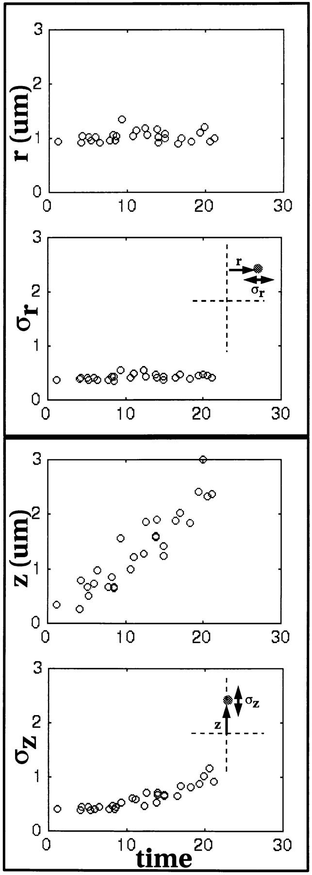
Characterization of the temporal changes in the distribution of histone loci in cycle 14 interphase nuclei for use in obtaining simulation boundaries. The top two panels report the average radial position (r) and its variance (σr) for the histone locus as a means to characterize histone's radial distribution in cycle 14 interphase. Note that the average radial position and the variance remain relatively constant throughout the observed portion of cycle 14 interphase. The bottom two panels report the average vertical position (z) and its variance (σz) for the histone locus. Here, the average vertical position increases but the variance remains relatively constant. The increasing average vertical position reflects the fact that the nuclei are lengthening. However, since the variance remains relatively constant, this indicates that volume over which the loci occupy remain relatively the same and that no significant spreading effect is caused by the upward movement of the locus. In the simulation, the normal distributions are generated based on variances measured at the earliest timepoints. Volume for the simulations is calculated from these variances as described in Materials and Methods.
The result of using such simulations to characterize the behavior of the pairing of the histone loci is given in Fig. 6 for changes in pairing frequency and inter-homologue distances, both for the case of diffusional motion and directed motion at constant velocity. Profiles for both the frequency of pairing and the inter-homologue distance as a function of time have been plotted for several values of the diffusion coefficient and velocity (Fig. 6, B and C). As might be expected, the time profiles for the frequency of pairing show a more gradual approach towards the completion of pairing in the random walk model (Fig. 6 B, top) as compared with the faster approach predicted by the model using directed motion (Fig. 6 C, top). Similarly, for time profiles expressing the changes in inter-homologue distance, we also see qualitatively distinct behavior for the different models. In the case of random walk, as sites that are near each other pair and are no longer included in the calculation of average distance between unpaired homologous sites, we intuitively expect that the average inter- homologue distance should shift to greater distances with time, while also showing the distances leveling off after longer time periods as a result of the imposed spatial confinement. The bottom panel of Fig. 6 B clearly demonstrates that this, indeed, is the case for this simulation. In contrast, we would expect an entirely different behavior for the inter-homologue distances based on a directed motion model. Here, as shown in the bottom panel of Fig. 6 C, the average distance between homologous sites should monotonically decrease, since by this model, sites are being pulled together at a constant velocity.
We then compared the actual measured profiles of histone pairing with those generated by the simulations. We only found good correlation in the pairing frequency plot between the experimental data and the simulations when motion is predicted to occur by a constrained random walk with a diffusion coefficient of D = 1.0 × 10⁻¹¹ cm2/s (Fig. 6 B, top). In contrast, the shape of the pairing frequency plots for the directed motion model did not fit the experimental data for any value of velocity (Fig. 6 C, top). When comparing actual and simulated inter-homologue distances (Fig. 6 B, bottom), the experimentally derived values again agreed only in the case when motion is modeled as a random walk where both the simulation and actual data show an increasing distance between unpaired loci with elapsed time. In contrast, when the measured profiles of histone pairing were compared with those obtained from the simulations based on the directed motion model (Fig. 6 C), little correspondence could be detected. This is particularly evident in the plots of inter-homologue distance (Fig. 6 C, bottom) where the simulations predict a decrease in the distance whereas the actual data shows a distinct increase. From these comparisons, we thus conclude that the pairing behavior of the histone locus is consistent with a random walk model for chromatin motion.
Perturbation of Pairing as a Consequence of Chromosome Rearrangement
The lt×13 strain (Wakimoto and Hearn, 1990) contains a reciprocal translocation between the centromeric heterochromatin on chromosome arm 2L and a subtelomeric site on arm 3R that moves the entire histone locus near the end of 3R (Fig. 8 A). Surprisingly, in strains homozygous for the lt×13 chromosome translocation, pairing levels for the histone locus during cycle 14 was found to be ∼30% on average compared with ∼70% for wild type (Hiraoka et al., 1993). In this strain, the average vertical position of the histone locus measured at the beginning of cycle 14 is shifted from the center of the nucleus (as seen in wild-type strains) to a position ∼1.5 μm lower. Why this positional change would result in much lower levels of histone pairing was never clear given that both loci are shifted equally in this homozygous translocation. Could it be that the intrinsic pairing ability of the histone locus is somehow affected by this translocation? One possibility would be that histone pairing is aided by other pairing sites and that the translocation removes it from these sites. This seems unlikely given the independence of the histone pairing from neighboring sites as shown earlier in this paper and the fact that high levels of pairing (83%) are again seen at the 13 h AED timepoint. Another possibility is that the translocation alters the chromosome context of the histone locus, for example, by separating it from regulatory domains linked in cis. Although this is a formal possibility, we note that the breakpoint in this translocation is not in, or even near, the histone locus, and so the flanking chromatin around the histone locus is likely to be the same in the translocated histone locus. An alternate explanation is that the large-scale nuclear positioning of the histone locus may be different in the translocation. In the Hiraoka study (Hiraoka et al. 1993), a plot of the distribution of histone loci for the wild-type and homozygous lt×13 strain revealed a slightly wider range in the distribution for the lt×13 strain. Given that histone pairing occurs by diffusion, the fact that histone loci now start farther apart on average may explain why, granted the same amount of time, pairing levels for the lt×13 strain are lower. To test this possibility, we measured the initial variances in the radial and vertical positions for the lt×13 (σro = 1.1 and σzo = 1.7; compare with wild type, σro = 0.4 and σzo = 0.4) and used simulations to predict the pairing behavior. The resulting profile (Fig. 8 B) shows that given this initial distribution of histone loci, a lowered pairing frequency is indeed expected. Moreover, similar levels of pairing were observed here (for t = 15 min, pairing level = 40% for lt×13; compare this to 70% for wild type as were seen in the Hiraoka study (Hiraoka et al. 1993; ∼30% for lt×13 and ∼70% for wild type). The slight discrepancy between the pairing levels for lt×13 from the different studies, 40 vs 30%, is most likely attributed to the fact that, in the Hiraoka study, no attempts were made to distinguish between embryos at different elapsed times in cycle 14. From these results, we conclude that the inherent pairing ability of the histone locus is not affected by the translocation, but rather, the wider distribution (i.e., larger variance) imposed by histone's new location is responsible for the lower frequency of pairing seen in these strains. This result, moreover, dramatically confirms the predictive power of the constrained random walk model, further increasing our confidence in its validity.
Figure 8.

Effects of chromosome rearrangement on the establishment of pairing. (A) Diagram illustrating chromosome arm 2L in a homozygous wild-type strain and in a homozygous lt×13 strain where 2L is translocated to the end of 3R. The dark filled areas indicate heterochromatic regions. The cross-hatched areas indicate approximate location of the histone locus. (B) Plot of the simulated pairing frequency for the histone locus in a lt×13 strain as a function of elapsed time in cycle 14. The experimentally determined pairing frequency for the histone locus in wild-type strain from Fig. 5 is plotted as empty circles. Plots were generated using actual experimental data for the initial distribution of the histone locus. D = 1.0 × 10⁻¹¹ cm2/s was used for the diffusion coefficient. Note that the pairing frequency is predicted to be much lower in the lt×13 strain than in the wild type (compare with Fig. 6 B, D = 1.0 × 10⁻¹¹ cm2/s).
Disruption of Pairing By Mitosis
To determine whether the pairing interactions are maintained throughout the cell cycle, we examined the level of histone pairing at different mitotic stages. During mitosis, several forces act upon chromosomes eventually resulting in chromosome separation to opposite poles (reviewed in Gorbsky, 1992). These forces include chromosome condensation, forces involved in metaphase congression and forces contributing to anaphase separation, all of which could potentially disrupt any homologous pairing associations formed in the preceding interphase. Evidence that pairing is indeed disrupted during mitosis is indicated here by the observation of a decrease in pairing levels for the histone locus in the transition between cycle 13 and cycle 14 interphase. At cycle 13 interphase, the average pairing frequency for this locus is 62% (Fig. 3) but at the beginning of cycle 14 interphase, the pairing level is down to 22% (Fig. 5 A). The reduction of the pairing level to 22% suggests that homologous pairing is completely dissociated during passage through mitosis. To further narrow down the timing of this disruption, we examined the pairing levels for the histone locus at selected stages of cycle 13 mitosis. During metaphase of cycle 13, when the chromosomes are maximally condensed, the association level for the histone locus is 63% (Fig. 9 A). Since these values are equivalent to what is found during cycle 13 interphase, disruption of the pairing association has not occurred up to this point. Note that no gain in the pairing levels is seen either, indicating that no significant pairing is occurring during passage through the prophase (50%) and metaphase stages. Next, we examined nuclei undergoing anaphase and here a dramatic disruption in the pairing was observed (Fig. 9 B). Anaphase figures were found with 4 (72%), 3 (18%), or 2 (10%) FISH signals for the histone locus. Up to four signals are seen in anaphase due to sister chromatid separation unlike the one or two signals found during metaphase when sister chromatids are still associated. Because each anaphase figure eventually results in two telophase nuclei, we counted each set of sister chromosomes as a separate nucleus in our calculation of pairing frequency in order to take into account any anaphase figures with three FISH signals (one paired, one unpaired). This results in a pairing frequency of 19% for the histone locus at anaphase. We conclude that it is during anaphase that pairing interactions are dissociated thus explaining the low levels of pairing frequency found at the beginning of cycle 14 interphase.
Figure 9.

Perturbation of pairing occurs at anaphase. (A) A volume-rendered image of metaphase chromosomes in several nuclei from a cycle 13 embryo overlaid with FISH signals from the histone probe. A 3-D data stack was projected down the optical (z) axis to create the volume rendered image. Over half the nuclei show a single FISH signal indicating that pairing of the histone locus is maintained. (B) A volume-rendered image of anaphase figures in several nuclei from a cycle 13 embryo overlaid with FISH signals from the histone probe. Here most anaphase figures display four FISH signals showing that pairing has been disrupted during this stage.
Discussion
Mechanism For Homologue Pairing
Greatly differing views exist for the mechanism whereby chromosomes find their homologous partners. On one hand, there are several models that propose active movements on the part of chromosomes to bring homologous sites together. Holliday (1968) postulated early on that one way for homologues to be drawn together is through the contraction of fibrillar connectors extending between specific DNA sequences on homologous chromosomes. A similar proposal was offered by Maguire (1983a) based on observations of homologous alignment at a distance (Maguire 1983b ) and on reports of the existence of premeiotic and early meiotic intranuclear bundles of microfilaments in microsporocytes (Bennett et al., 1979). More recently, Kleckner et al. (1991), modifying a proposal by Smithies and Powers (1986), alternatively favored the view that after the initial formation of unstable DNA-DNA interactions through chance encounters, chromosome condensation may further drive homologues closer together. A common feature in all of the aforementioned models is that at some point homologous regions are directed towards each other. This is in contrast to the opposing view that random contacts of homologous sequences, brought about by diffusion of chromatin, is the primary mode in establishing homologous pairing (e.g., Brown and Stack, 1968).
In this study, we provide the first demonstration of the means by which pairing takes place. By measuring the actual kinetics of pairing and using simulations based on directed and random walk models, we show that pairing of the histone locus during Drosophila embryonic development is consistent with a mechanism that relies on finding a homologous locus through diffusive motion of the chromatin.
The occurrence of random walk motion of chromatin during interphase has been confirmed in several organisms. Recently, Marshall et al. (1997) directly measured chromatin motion in live interphase nuclei in Drosophila and budding yeast and found in all cases that the observed loci moved by random walk motion. The diffusion coefficient, D = 1.0 × 10⁻¹¹ cm2/s that we obtained from our pairing analysis is in excellent agreement with D = 1.25 × 10⁻¹¹ cm2/s obtained in the Marshall et al. (1997) study directly measuring chromatin motion in living Drosophila embryonic nuclei. Although the 359-bp satellite repeat on chromosome X and not the histone locus was analyzed in the case of Drosophila, the diffusion coefficient obtained for this locus corresponded well with the value acquired by our analysis of the histone pairing profile. Even apart from simulations, it can be seen that the magnitude of the diffusion constant reported by Marshall et al. (1997) is roughly consistent with the spatial and temporal scale of the homologue pairing problem. As a crude calculation, we recognize that the mean squared change in the mutual distance r between two diffusing loci is given by the equation < r 2 > = 4Dt (von Smoluchowski, 1917). Thus in 10 min, given a diffusion constant on the order of 10−11 cm2/s (Marshall et al., 1997), the two spots would move towards or away from each other by an average distance of ∼1.5 μm. Thus the micron-scale movements required for homologue pairing are predicted to take place on roughly the 10-min time scale, consistent with the duration of interphase. The fact that the diffusion coefficient obtained from the histone pairing profile agrees with the value obtained in the independent study of chromatin motion in Drosophila gives further support that pairing of the histone locus does indeed occur via random walk motion of chromatin.
Although this study strongly suggests a diffusion-driven random walk mechanism for homologue pairing, there may be other mechanisms that pair other sites. There still could be a combination of mechanisms including condensation and/or active processes that also play important roles in achieving full homologous association. Active movement of telomere-led chromosome motions that occur preceding meiosis in fission yeast (Chikashige et al., 1994) may be one example of how active processes may be used to create conditions that promote the homology search.
Is Pairing Permanent or Transient?
Our model for attainment of pairing by a random walk search makes the assumption that once two homologous loci encounter each other and pair, that they subsequently remain paired and do not dissociate. In this model, differences in pairing levels between different loci reflect differences in the rates at which pairing is first attained. However, an alternate possibility to this kinetic model would be transient pairing followed by dissociation, with the observed pairing levels reflecting the equilibrium balance between association and dissociation. Indeed, it has been pointed out by Kleckner and Weiner (1993) that such a transient pairing could be advantageous in resolving interlocks during meiotic homologue pairing.
Clearly, because pairing levels of the histone locus increase continuously during the first 20 min of cycle 14 interphase, any equilibrium that is attained must take at least 20 min. Indeed, it must take even longer since attainment of maximum pairing levels takes even more time for other loci. Thus, during this time frame it cannot be the case that differences in pairing levels simply reflect equilibrium balance of association and dissociation, as a steady state has not yet been reached. Nevertheless, although we can thus conclude that differences in pairing are the result of kinetic, rather than equilibrium differences, it is still a formal possibility that some of the paired loci can dissociate, even though they must do so much less frequently than they associate (otherwise pairing levels would not increase). To test this idea we consider the predicted consequences of the transient pairing model on the behavior of the average distance between unpaired loci versus time. Transient pairing predicts that there are two types of unpaired sites: sites that have never paired, and sites that have paired but dissociated. Sites that have never paired will be distributed the same way as all the sites were at the beginning of interphase, i.e., randomly. But unpaired sites generated by dissociation of paired sites will not be randomly distributed but will on the contrary be much closer together, since they had recently been overlapping and only a limited time has passed during which they can diffuse apart. Assuming that the dissociation, like standard macromolecular dissociations, is a first order process with respect to the number of paired loci, then the number of unpaired loci resulting from dissociation will be directly proportional to the number of paired loci at any given time. This would predict then that as the frequency of paired sites increases over time, that the fraction of unpaired sites generated by dissociation would similarly increase, and because such pairs of sites are nonrandomly close together, therefore the average distance between unpaired loci is predicted to decrease. But in fact our data indicates that the distance between unpaired loci actually increases over time. Therefore, we conclude that dissociation of paired loci, if it happens at all, must be a rather low probability event and therefore the pairing we observe is not an equilibrium association/dissociation process, but rather an irreversible adsorption process, with paired loci remaining paired more or less permanently. Whether or not this will also be true of meiotic homologue pairing remains to be determined.
Disruption of Pairing Interactions by Mitosis
Our histone results indicate that pairing interactions begin to form at the start of interphase. During interphase when pairing is in progress, chromosomes are at their most decondensed state, in agreement with previous suggestions that pairing occurs when chromatin is not greatly compacted (Kleckner et al., 1991; Dawe et al., 1994). During this time, S phase, DNA replication, and histone gene transcription also occur concomitantly (Edgar and Schubiger, 1986; Edgar and O'Farrell, 1990) with no obvious interference to the pairing interactions. Nor is there any disruption due to forces involved in chromosome condensation or metaphase congression as seen by the maintenance in pairing levels up to the metaphase stage. Consequently, we believe that relatively strong interactions are created between the two homologous regions when they contact, which in mitosis, are only disrupted during anaphase. A possible explanation for this disruption is that spindle forces acting to segregate the sister chromatids to opposite poles somehow exert enough force or create enough agitation to cause dissociation of homologous pairing. For example suppose that each chromatid of one homologue interacts with just one chromatid of the other homologue. To maintain pairing, the kinetochores on these two homologous chromatids must segregate to the same pole, and if, due to random segregation of sister kinetochores, they segregate to opposite poles, clearly homologous pairing will be disrupted. We consider this to be a very likely possibility. However, it is also possible that the same factors regulating the end of sister chromatid cohesion may also release homologous associations.
The fact that anaphase almost completely disrupts the pairing formed during the previous interphase has bearing on the proposed concept of graduality in the pairing process. It has been suggested that meiotic pairing results from gradually increasing the number of loci that are paired over the course of several cell cycles preceding meiosis (Brown and Stack, 1968). However, if it is true that complete disruption of pairing interactions occurs at every mitosis, no significant accumulation of pairing should be obtained from successive cell cycles. Rather, in order for pairing to be established over long stretches of chromatin, it seems that a long interphase or an uninterrupted period during which chromosomes are still decondensed is required, particularly if part or all of the pairing is to occur by random walk motion. The importance of the length of the cell cycle has been previously stressed by Golic and Golic (1996). In their study, they found that minute mutations that significantly slow the rate of cell division in imaginal discs could suppress the effects of rearrangements on transvection. A longer period where chromosomes are still decondensed also coincides nicely with observations in several organisms that the duration of premeiotic interphase (Bennett et al., 1973; Williamson et al., 1983) and prophase I (reviewed in Bennett, 1977) are quite lengthy in comparison to their mitotic counterparts. We must point out that although we observe homologues to dissociate during anaphase, it remains a formal possibility that some invisible connection remains between them that allows them to reestablish pairing more efficiently in the next interphase. Such a persistent linkage would allow for gradual attainment of pairing over multiple cell cycles. However, since there is at present no evidence whatsoever for such a linkage, we consider this possibility to be remote.
Reevaluation of the Onset of Pairing for the Histone Locus
The requirement for a sufficiently long interphase period may also explain why in early nuclear divisions of Drosophila embryogenesis the level of pairing of the histone locus on average is much lower than the level seen at cycle 14 (Hiraoka et al., 1993). The dramatic change in the level of histone pairing at cycle 14 was used to propose that the histone locus had the capability to pair only after the transition to cycle 14. We now believe that it is timing and not competence for pairing that explains the change in pairing levels. We propose that the pairing capability for the histone locus exists for all cell cycles, but that the shorter cell cycle times for early divisions (e.g., cycle 12, 13 min; cycle 13, 17 min, times include mitosis (Foe and Alberts, 1983), do not allow sufficient time to achieve high levels of pairing. Corroborating evidence is that the cycle 13 pairing frequency of 61% measured in this study (Fig. 3) shows that the histone locus, indeed, becomes paired before the transition to cycle 14. One possibility why only a 32% pairing frequency for cycle 13 was seen in the previous work may be that only earlier cycle 13 embryos were examined due to differences in the collection temperature, leading to the impression of a very sharp change in the pairing frequency at the transition between cycle 13 and 14.
What Governs the Ability of Homologues to Pair?
The variation in the temporal pattern of the attainment of pairing seen during Drosophila development in this study raises the question why certain sites attain high levels of pairing very early in development whereas other sites take much longer. This question can be said to relate to the more general issue of what might govern the ability for homologous sites to pair. An answer to this question will not only help us understand how pairing develops to the point that a whole chromosome is completely aligned but will also help us comprehend observations that in most somatic tissues, except in the case of Dipterans, homologous pairing specifically occurs for some loci but not for others. For a long time, conflicting evidence existed whether somatic pairing, outside what was seen for Dipteran insects, occurred at all (Haaf and Schmid, 1991). However, recent evidence now indicates that somatic pairing does occur in a site-specific manner and that the contradictory results obtained previously arose from the fact that such pairing is highly dependent on the particular tissue being examined and the time frame being studied. For example, using 3-D FISH techniques combined with fluorescence-activated cell sorting, LaSalle and Lalande (1996) found in human lymphocytes that homologous association occurred specifically at the imprinted 15q11-q13 regions only during late S phase of the cell cycle. A related observation was made for the existence of a tissue dependence for somatic pairing in earlier work by Arnoldus et al. (1989) showing that homologous association is detected for human chromosome 1 from nuclei taken from cerebellar tissue but not in nuclei from cerebral tissue. Even in Drosophila, where somatic homologue pairing is complete in many cases, there is also evidence suggesting inherent differences in pairing ability of different loci in meiosis (McKee et al., 1993). For example, McKee et al. (1993) examining the distribution of autosomal pairing ability in Drosophila males during meiosis by characterizing the pairing and segregation patterns of males carrying various transpositions of regions derived from chromosome 2 into Y, identified a strong pairing site found to contain the histone locus. Other studies focusing instead on the sex chromosomes show that the rDNA locus is a strong pairing site as well (reviewed in McKee, 1996). Thus in many organisms, it appears that different sites have different inherent tendencies to homologously pair, but the basis for these differences is currently unknown.
In this paper, we have examined and eliminated several possibilities as reasons why certain sites may demonstrate preferential pairing abilities over others. In the two loci that paired the earliest, histone and Rsp, a common feature in both is that each locus consists of several repetitions of their respective sequence. However, examination of other loci with repeated sequences (e.g., AACAC) show quite clearly that repetition alone is not sufficient to confer early participation in the pairing process. Although it was possible that there could be fundamental differences in pairing at euchromatic and heterochromatic loci, the careful, systematic comparison performed here shows no consistent differences.
There remain several possible explanations for differences in pairing ability. One suggestion is that transcriptional activity may also correlate with pairing ability (McKee, 1996) since both the histone and rDNA loci, found to be strong pairing sites during male meiosis are also known to be highly transcribed. However, it is unclear whether the heterochromatic Rsp locus, one of the earliest pairing sites in the embryo, is even transcribed. The correlation between transcription and pairing is thus far from compelling. Another possibility is that differences in pairing could arise from differences in protein-binding sites at different loci. If homologue pairing is mediated by chromatin-associated proteins, then differences in the affinity of these proteins for certain regions will be reflected in differences in the propensity for those regions to pair. Thus, the explanation for differences in pairing ability remains an open question requiring further investigation.
The Role of Nuclear Organization in Homologue Pairing
From our profile of the pairing frequency for the histone locus, we found experimentally that pairing can occur at a significant rate, such that, by the first 20 min of cycle 14 interphase, 80% of the nuclei contain paired histone loci. It was also especially evident from monitoring histone pairing in the lt×13 strain, that the observed pairing frequencies strongly depend on the spatial probability distribution of each of the sites in the unpaired state. Thus, we would like to speculate that a key determinant of homologous pairing is the 3-D architecture of the nucleus. As discussed earlier, it has been shown that in the Drosophila early embryo a given locus occupies a discrete subregion within the nucleus (Marshall et al., 1996). This organization stems from a combination of an overall centromere–telomere spatial organization (the classical “Rabl” configuration), as well as more specific patterning. As a result, a given locus is found to occupy a disk- or annulus-shaped volume within the nucleus, whose vertical position depends on the distance from the centromere and whose radial extent is based on a consistent distance from the nuclear envelope (NE). In particular, a set of ∼10–15 sites per chromosome arm have been identified in the Drosophila embryo that are closely associated with the NE, whereas another set of sites have been identified that are nonrandomly localized to the interior of the nucleus. Homology search by any given locus will thus be confined to the small subregion in which it is localized. We propose that because both homologous copies of such a locus will, in general, occupy the same subregion, the homology search will be greatly facilitated. Moreover, time spent exploring nonhomologous loci will be greatly reduced, since most nonhomologous loci will be restricted to separate regions of the nucleus and will never come into contact during the pairing process. Thus, a highly defined nuclear architecture, such as is clearly seen in the Drosophila embryo, can dramatically enhance the rate of homology searching. We can carry this hypothesis one step further: computer simulations in this study indicate that the rate of homology searching depends critically on both the initial distance between the loci and the size of the region in which the search takes place. Loci with more peripheral localizations will be found within a significantly larger annular region than loci positioned more internally, and thus the homology search should take longer. Thus, we predict that the sites that pair first will be those that are most internally localized. Interestingly, both histone and Rsp, the first sites to pair on chromosome 2, are nonrandomly internal (Marshall et al., 1996), indeed they are the only such sites known on chromosome 2. A picture is thus emerging in which position within the nucleus, as specified via the nuclear architecture, plays a critical role in homologue pairing, and could in fact explain why some sites pair much earlier than others.
Abbreviations used in this paper
- 3-D
three-dimensional
- AED
after egg deposition
- FISH
fluorescence in situ hybridization
- NE
nuclear envelope
- Rsp
responder
Footnotes
Jennifer C. Fung and Wallace F. Marshall's present address is MCDB Dept., Yale University, New Haven, CT 06520.
Abby Dernburg's present address is Department of Developmental Biology, Stanford University School of Medicine, Palo Alto, CA 94305.
References
- Agard DA, Hiraoka Y, Shaw P, Sedat JW. Fluorescence microscopy in three dimensions. Methods Cell Biol. 1989;30:353–377. doi: 10.1016/s0091-679x(08)60986-3. [DOI] [PubMed] [Google Scholar]
- Aramayo R, Metzenberg RL. Meiotic transvection in fungi. Cell. 1996;86:103–113. doi: 10.1016/s0092-8674(00)80081-1. [DOI] [PubMed] [Google Scholar]
- Arnoldus EP, Peters AC, Bots GT, Raap AK, van der Ploeg M. Somatic pairing of chromosome 1 centromeres in interphase nuclei of human cerebellum. Hum Genet. 1989;83:231–234. doi: 10.1007/BF00285162. [DOI] [PubMed] [Google Scholar]
- Ashburner, M. 1989. Drosophila. Cold Spring Harbor Laboratory, Cold Spring Harbor, NY. 380 pp.
- Bennett MD. The timing and duration of meiosis. Phil Trans R Soc Lond Ser B. 1977;277:201–226. doi: 10.1098/rstb.1977.0012. [DOI] [PubMed] [Google Scholar]
- Bennett MD, Rao MK, Smith JB, Bayliss MW. Cell development in the anther, ovule, and young seed of Triticum aestivum L. cv. Chinese Spring. Phil Trans R Soc Ser B. 1973;266:39–81. [Google Scholar]
- Bennett MD, Smith JB, Simpson S, Wells B. Intranuclear fibrillar material in cereal pollen mother cells. Chromosoma. 1979;71:289–332. [Google Scholar]
- Berg, H.C. 1983 Random walks in biology. Princeton University Press, Princeton. 5–36.
- Bollmann J, Carpenter R, Coen ES. Allelic interactions at the nivea locus of Antirrhinum. Plant Cell. 1991;3:1327–1336. doi: 10.1105/tpc.3.12.1327. [DOI] [PMC free article] [PubMed] [Google Scholar]
- Brown WV, Stack SM. Somatic pairing as a regular preliminary to meiosis. Bull Torrey Bot Club. 1968;95:369–378. [Google Scholar]
- Chen H, Hughes DD, Chan TA, Sedat JW, Agard DA. IVE image visualization environment—a software platform for all three-dimensional microscopy applications. J Struct Biol. 1996;116:56–60. doi: 10.1006/jsbi.1996.0010. [DOI] [PubMed] [Google Scholar]
- Chikashige Y, Ding DQ, Funabiki H, Haraguchi T, Mashiko S, Yanagida M, Hiraoka Y. Telomere-led premeiotic chromosome movement in fission yeast. Science. 1994;264:270–273. doi: 10.1126/science.8146661. [DOI] [PubMed] [Google Scholar]
- Colot V, Maloisel L, Rossignol JL. Interchromosomal transfer of epigenetic states in ascobolus—transfer of DNA methylation is mechanistically related to homologous recombination. Cell. 1996;86:855–864. doi: 10.1016/s0092-8674(00)80161-0. [DOI] [PubMed] [Google Scholar]
- Crank, J. 1956. The mathematics of diffusion. Clarendon Press, Oxford.
- Dawe RK, Sedat JW, Agard DA, Cande WZ. Meiotic chromosome pairing in maize is associated with a novel chromatin organization. Cell. 1994;76:901–912. doi: 10.1016/0092-8674(94)90364-6. [DOI] [PubMed] [Google Scholar]
- Dernburg, A.F., and J.W. Sedat. 1997. Mapping three-dimensional chromosome architecture in situ. In Methods in Cell Biology. M. Barrios, editor. Academic Press, NY. 187–233. [DOI] [PubMed]
- Dernburg, A.F., J.W. Sedat, W.Z. Cande, and H.W. Bass. 1995. Cytology of Telomeres. In Telomeres. E.H. Blackburn and C.W. Greider, editors. Cold Spring Harbor Laboratory, Plainview, NY. 295–338.
- Dernburg AF, Daily DR, Yook KJ, Corbin JA, Sedat JW, Sullivan W. Selective loss of sperm bearing a compound chromosome in the Drosophilafemale. Genetics. 1996;143:1629–1642. doi: 10.1093/genetics/143.4.1629. [DOI] [PMC free article] [PubMed] [Google Scholar]
- Dorninger D, Karigl G, Loidl J. Simulation of chromosomal homology searching in meiotic pairing. J Theor Biol. 1995;176:247–260. doi: 10.1006/jtbi.1995.0195. [DOI] [PubMed] [Google Scholar]
- Edgar BA, Schubiger G. Parameters controlling transcriptional activation during early Drosophiladevelopment. Cell. 1986;44:871–877. doi: 10.1016/0092-8674(86)90009-7. [DOI] [PubMed] [Google Scholar]
- Edgar BA, O'Farrell PH. The three postblastoderm cell cycles of Drosophilaembryogenesis are regulated in G2 by string. Cell. 1990;62:469–480. doi: 10.1016/0092-8674(90)90012-4. [DOI] [PMC free article] [PubMed] [Google Scholar]
- Foe VE. Mitotic domains reveal early commitment of cells in Drosophilaembryos. Development (Camb) 1989;107:1–22. [PubMed] [Google Scholar]
- Foe VE, Alberts BM. Studies of nuclear and cytoplasmic behaviour during the five mitotic cycles that precede gastrulation in Drosophilaembryogenesis. J Cell Sci. 1983;61:31–70. doi: 10.1242/jcs.61.1.31. [DOI] [PubMed] [Google Scholar]
- Foe VE, Alberts BM. Reversible chromosome condensation induced in Drosophilaembryos by anoxia: visualization of interphase nuclear organization. J Cell Biol. 1985;100:1623–1636. doi: 10.1083/jcb.100.5.1623. [DOI] [PMC free article] [PubMed] [Google Scholar]
- Foe, V.E., G.M. Odell, and B.A. Edgar. 1993. Mitosis and morphogenesis in the Drosophila embryo. In The development of Drosophila melanogaster. M. Bate and A. Martinez Arias, editors. Cold Spring Harbor Laboratory Press, Plainview, NY. 149–300.
- Fussell, C.P. 1987. The Rabl orientation: a prelude to synapsis. In Meiosis. P.B. Moens, editor. Academic Press, Orlando, Florida. 275–288.
- Goldsborough AS, Kornberg TB. Reduction of transcription by homologue asynapsis in Drosophilaimaginal discs. Nature. 1996;381:807–810. doi: 10.1038/381807a0. [DOI] [PubMed] [Google Scholar]
- Golic KG, Golic MM. A quantitative measure of the mitotic pairing of alleles of Drosophila melanogasterand the influence of structural heterozygosity. Genetics. 1996;143:385–400. doi: 10.1093/genetics/143.1.385. [DOI] [PMC free article] [PubMed] [Google Scholar]
- Gorbsky GJ. Chromosome motion in mitosis. Bioessays. 1992;14:73–80. doi: 10.1002/bies.950140202. [DOI] [PubMed] [Google Scholar]
- Haaf T, Schmid M. Chromosome topology in mammalian interphase nuclei. Exp Cell Res. 1991;192:325–332. doi: 10.1016/0014-4827(91)90048-y. [DOI] [PubMed] [Google Scholar]
- Hartl DL, Nurminsky DI, Jones RW, Lozovskaya ER. Genome structure and evolution in Drosophila: applications of the framework P1 map. Proc Natl Acad Sci USA. 1994;91:6824–6829. doi: 10.1073/pnas.91.15.6824. [DOI] [PMC free article] [PubMed] [Google Scholar]
- Heino TI, Sauro AO, Sorsa V. Maps of salivary gland chromosomes of D. melanogaster. . Drosophila Information Source. 1994;73:73–621. [Google Scholar]
- Hiraoka Y, Swedlow JR, Paddy MR, Agard DA, Sedat JW. Three-dimensional multi-wavelength fluorescence microscopy for the structural analysis of biological phenomena. Semin Cell Biol. 1991;2:153–165. [PubMed] [Google Scholar]
- Hiraoka Y, Dernburg AF, Parmelee SJ, Rykowski MC, Agard DA, Sedat JW. The onset of homologous chromosome pairing during Drosophila melanogasterembryogenesis. J Cell Biol. 1993;120:591–600. doi: 10.1083/jcb.120.3.591. [DOI] [PMC free article] [PubMed] [Google Scholar]
- Holliday, R. 1968. Genetic recombination in fungi. In Replication and Recombination of Genetic Material. W.J. Peacock and R.D. Brock, editors. Australian Academy of Science, Canberra. 157–174.
- Kalpin RF, Daily DR, Sullivan W. Use of dextran beads for live analysis of the nuclear division and nuclear envelope breakdown/reformation cycles in the Drosophilaembryo. Biotechniques. 1994;17:732–733. [PubMed] [Google Scholar]
- Kao HP, Verkman AS. Tracking of single fluorescent particles in three dimensions: use of cylindrical optics to encode particle position. Biophys J. 1994;67:1291–1300. doi: 10.1016/S0006-3495(94)80601-0. [DOI] [PMC free article] [PubMed] [Google Scholar]
- Kleckner N, Weiner BM. Potential advantages of unstable interactions for pairing of chromosomes in meiotic, somatic, and premeiotic cells. Cold Spring Harbor Symp Quant Biol. 1993;58:553–565. doi: 10.1101/sqb.1993.058.01.062. [DOI] [PubMed] [Google Scholar]
- Kleckner N, Padmore R, Bishop DK. Meiotic chromosome metabolism: one view. Cold Spring Harbor Symp Quant Biol. 1991;56:729–743. doi: 10.1101/sqb.1991.056.01.082. [DOI] [PubMed] [Google Scholar]
- LaSalle JM, Lalande M. Homologous association of oppositely imprinted chromosomal domains. Science. 1996;272:725–728. doi: 10.1126/science.272.5262.725. [DOI] [PubMed] [Google Scholar]
- Lewis EB. The theory and application of a new method of detecting chromosomal rearrangements in Drosophila melanogaster. . Am Nat. 1954;88:225–239. [Google Scholar]
- Lewis JP, Tanke HJ, Raap AK, Beverstock GC, Kluin-Nelemans HC. Somatic pairing of centromeres and short arms of chromosome 15 in the hematopoietic and lymphoid system. Hum Genet. 1993;92:577–582. doi: 10.1007/BF00420942. [DOI] [PubMed] [Google Scholar]
- Lifton RP, Goldberg ML, Karp RW, Hogness DS. The organization of the histone genes in Drosophila melanogaster: function and evolutionary implications. Cold Spring Harbor Symp Quant Biol. 1977;42:1047–1051. doi: 10.1101/sqb.1978.042.01.105. [DOI] [PubMed] [Google Scholar]
- Lohe AR, Hilliker AJ, Roberts PA. Mapping simple repeated DNA sequences in heterochromatin of Drosophila melanogaster. . Genetics. 1993;134:1149–1174. doi: 10.1093/genetics/134.4.1149. [DOI] [PMC free article] [PubMed] [Google Scholar]
- Loidl J. The initiation of meiotic chromosome pairing: the cytological view. Genome. 1990;33:759–778. doi: 10.1139/g90-115. [DOI] [PubMed] [Google Scholar]
- Loidl J, Langer H. Evaluation of models of homologue search with respect to their efficiency on meiotic pairing. Heredity. 1993;71:342–351. doi: 10.1038/hdy.1993.148. [DOI] [PubMed] [Google Scholar]
- Maguire M. Chromosome behavior at premeiotic mitosis in maize. J Hered. 1983a;74:93–96. [Google Scholar]
- Maguire M. Homologous chromosome pairing remains an unsolved problem: a test of a popular hypothesis utilizing maize meiosis. Genetics. 1983b;104:173–179. doi: 10.1093/genetics/104.1.173. [DOI] [PMC free article] [PubMed] [Google Scholar]
- Marshall WF, Dernburg AF, Harmon B, Agard DA, Sedat JW. Specific interactions of chromatin with the nuclear envelope—positional determination within the nucleus in Drosophila melanogaster. . Mol Biol Cell. 1996;7:825–842. doi: 10.1091/mbc.7.5.825. [DOI] [PMC free article] [PubMed] [Google Scholar]
- Marshall WF, Straight A, Marko JF, Swedlow JR, Dernburg AF, Belmont BA, Murray AW, Agard DA, Sedat JW. Interphase chromosomes undergo constrained diffusional motion in living cells. Curr Biol. 1997;7:930–939. doi: 10.1016/s0960-9822(06)00412-x. [DOI] [PubMed] [Google Scholar]
- McKee BD. The license to pair—identification of meiotic pairing sites in Drosophila. . Chromosoma. 1996;105:135–141. doi: 10.1007/BF02509494. [DOI] [PubMed] [Google Scholar]
- McKee BD, Lumsden SE, Das S. The distribution of male meiotic pairing sites on chromosome 2 of Drosophila melanogaster: meiotic pairing and segregation of 2-Y transpositions. Chromosoma. 1993;102:180–194. doi: 10.1007/BF00387733. [DOI] [PubMed] [Google Scholar]
- Metz CW. Chromosome studies on the Diptera II. The paired association of chromosomes in the Diptera and its significance. J Exp Zool. 1916;21:213–279. [Google Scholar]
- Minden JS, Agard DA, Sedat JW, Alberts BM. Direct cell lineage analysis in Drosophila melanogasterby time lapse three dimensional optical microscopy of living cells. J Cell Biol. 1989;109:505–516. doi: 10.1083/jcb.109.2.505. [DOI] [PMC free article] [PubMed] [Google Scholar]
- Paddy MR, Belmont AS, Saumweber H, Agard DA, Sedat JW. Interphase nuclear envelope lamins form a discontinuous network that interacts with only a fraction of the chromatin in the nuclear periphery. Cell. 1990;62:89–106. doi: 10.1016/0092-8674(90)90243-8. [DOI] [PubMed] [Google Scholar]
- Pardue, M.L. 1986. In situ hybridization to DNA of chromosomes and nuclei. IRL Press, Ltd., Oxford. 111–137.
- Patterson GI, Chandler VL. Paramutation in maize and related allelic interactions. Curr Top Microbiol Immunol. 1995;197:121–141. doi: 10.1007/978-3-642-79145-1_9. [DOI] [PubMed] [Google Scholar]
- Rabl C. Uber Zelltheilung. Morphol Jahrb. 1985;10:214–330. [Google Scholar]
- Roeder GS. Sex and the single cell—meiosis in yeast. Proc Natl Acad Sci USA. 1995;92:10450–10456. doi: 10.1073/pnas.92.23.10450. [DOI] [PMC free article] [PubMed] [Google Scholar]
- Scherthan HS, Weich SH, Harle M, Heyting C, Cremer T. Centromere and telomere movements during early meiotic prophase of mouse and man are associated with the onset of chromosome pairing. J Cell Biol. 1996;134:1109–1125. doi: 10.1083/jcb.134.5.1109. [DOI] [PMC free article] [PubMed] [Google Scholar]
- Smithies, O., and P.A. Powers. 1986. Gene conversions and their relation to homologous chromosome pairing. Philos. Trans. R. Soc. Lond. Ser. B: Biol. Sci. 312:291–302. [DOI] [PubMed]
- Smolik-Utlaut SM, Gelbart WM. The effects of chromosomal rearrangements on the zeste-white interaction in Drosophila melanogaster. . Genetics. 1987;116:285–298. doi: 10.1093/genetics/116.2.285. [DOI] [PMC free article] [PubMed] [Google Scholar]
- von Smoluchowski M. Versuch einer mathematischen Theorie der Koagulationskinetik kolloider Loesungen. Z Phys Chem. 1917;92:129–168. [Google Scholar]
- Tartof KD, Henikoff S. Trans-sensing effects from Drosophilato humans. Cell. 1991;65:201–203. doi: 10.1016/0092-8674(91)90153-p. [DOI] [PubMed] [Google Scholar]
- Vourc'h C, Taruscio D, Boyle AL, Ward DC. Cell cycle-dependent distribution of telomeres, centromeres, and chromosome-specific subsatellite domains in the interphase nucleus of mouse lymphocytes. Exp Cell Res. 1993;205:142–151. doi: 10.1006/excr.1993.1068. [DOI] [PubMed] [Google Scholar]
- Wakimoto BT, Hearn MG. The effects of chromosome rearrangements on the expression of heterochromatic genes in chromosome 2L of Drosophila melanogaster. . Genetics. 1990;125:141–154. doi: 10.1093/genetics/125.1.141. [DOI] [PMC free article] [PubMed] [Google Scholar]
- Williamson DH, Johnston LH, Fennell DJ, Simchen G. The timing of S phase and other nuclear events in yeast meiosis. Exp Cell Res. 1983;145:209–217. doi: 10.1016/s0014-4827(83)80022-6. [DOI] [PubMed] [Google Scholar]
- Zar, J.H. 1984. Biostatistical Analysis. Prentice Hall, Englewood Cliffs, NJ. 718 pp.