Effect of flexibility and cis residues in single-molecule FRET studies of polyproline

Abstract

Polyproline has recently been used as a spacer between donor and acceptor chromophores to help establish the accuracy of distances determined from single-molecule Förster resonance energy transfer (FRET) measurements. This work showed that the FRET efficiency in water is higher than expected for a rigid spacer and was attributed to the flexibility of the polypeptide. Here, we investigate this issue further, using a combination of single-molecule fluorescence intensity and lifetime measurements, NMR, theory, and molecular dynamics simulations of polyproline-20 that include the dyes and their linkers to the polypeptide. NMR shows that in water ≈30% of the molecules contain internal cis prolines, whereas none are detectable in trifluoroethanol. Simulations suggest that the all-trans form of polyproline is relatively stiff, with persistence lengths of 9–13 nm using different established force fields, and that the kinks arising from internal cis prolines are primarily responsible for the higher mean FRET efficiency in water. We show that the observed efficiency histograms and distributions of donor fluorescence lifetimes are explained by the presence of multiple species with efficiencies consistent with the simulations and populations determined by NMR. In calculating FRET efficiencies from the simulation, we find that the fluctuations of the chromophores, attached to long flexible linkers, also play an important role. A similar simulation approach suggests that the flexibility of the chromophore linkers is largely responsible for the previously unexplained high value of R₀ required to fit the data in the classic study of Stryer and Haugland.

Förster resonance energy transfer (FRET) has been a widely used tool for determining distances within and between biological molecules, and was called a “spectroscopic ruler” by Stryer and Haugland (1, 2). The basis of the technique is that the rate of energy transfer, k_ET, between two chromophores depends on their separation in space R according to k_ET = k_D(R₀/R)⁶, as shown by Förster (k_D⁻¹ is the fluorescence lifetime of the “donor” chromophore and R₀ the distance at 50% transfer efficiency). The prediction of an R⁻⁶ dependence of k_ET was initially confirmed in the experiment by Stryer and Haugland (1), who used a series of l-proline oligomers (Fig. 1A) as spacers of known length (3) between naphthyl and dansyl chromophores. Based on the early theoretical estimate by Schimmel and Flory (4) of 22 nm for the persistence length of poly-l-proline in the type II conformation, the spacers of 1–12 prolines were considered as rigid rods, resulting in a good fit of the theory to the experimental transfer efficiencies. An unexplained result, however, was that the fit required an R₀ significantly longer than the value determined spectroscopically.

Fig. 1.

Polyproline structures. Space-filling representation of polyproline-20 labeled with Alexa Fluor 488 (FRET donor) at the C-terminal cysteine and Alexa Fluor 594 (FRET acceptor) at the N-terminal glycine in the all-trans conformation (A) and with residue 8 (purple) in the cis conformation (B). (B Inset) A polyproline fragment with one cis peptide bond (shown as “ω = 0”). One of the remaining trans peptide bonds is also indicated (“ω = 180”).

Advances in detector technology and the use of fluorophores with very high extinction coefficients, large quantum yields, and photochemical stability have made it possible to measure FRET in single molecules (5). This development has enabled several single-molecule FRET studies of protein folding, aimed at obtaining information on intramolecular distance distributions as molecules fold (6–20). As a “control” for determining the accuracy of distances obtained from single-molecule FRET results, Schuler et al. (15) effectively repeated the Stryer and Haugland experiment at the single-molecule level on freely diffusing molecules with continuous wave laser excitation (15), using longer polyprolines of 6–40 residues because of the larger R₀ (5.4 nm) in their experiment. The FRET efficiencies of the oligomers with >17 residues were found to be much higher than expected for rigid polyproline. This effect was largely reproduced by implicit solvent simulations, and explained in terms of polyproline flexibility [a persistence length of 5 nm was obtained from the simulations, compared with the original estimate of 22 nm by Schimmel and Flory (4)]. Schuler et al. (15) also found that the width of the FRET efficiency distribution was greater than expected from shot noise, but did not investigate possible causes. In a subsequent study, Watkins et al. (21) measured single-molecule photon trajectories from continuous wave excitation of immobilized polyprolines of 8–24 residues. After correcting for shot noise, they concluded that there is a static distribution of different conformers of polyproline. Using a worm-like chain model, they calculated that a persistence length of 2.3 nm would be required to fit the observed mean efficiency. Watkins et al. (21) also suggested that the structure distribution resulted from the presence of cis prolines but made no estimate of their contribution.

Given the importance of experiments on polyproline for quantifying distance information in single-molecule FRET experiments, as well as the large variation in reported persistence lengths, we have investigated this problem further. We have used NMR spectroscopy to determine the fraction and location of cis prolines (Fig. 1B), measured single-molecule photon trajectories using pulsed, picosecond excitation of freely diffusing molecules to obtain accurate FRET efficiencies from the fluorescence decay curves of subpopulations, and performed molecular dynamics calculations to interpret the results. The single-molecule lifetime and intensity data are interpreted in terms of the NMR-determined populations of cis isomers and the efficiencies for these isomers obtained from molecular dynamics calculations that include the dyes and their linkers. To compare the FRET efficiency histograms with the predictions from the simulations, a theoretical model was used that accounts for both photon statistics and background noise. Measurements were also made in trifluoroethanol (TFE), believed to reduce the cis proline content relative to water (22).

Results

Fraction and Location of cis Residues in Polyproline Determined by NMR.

The H^α region of the ¹H spectra of polyproline-8 and polyproline-20 [(Pro)₈Gly and (Pro)₂₀Gly] in D₂O is shown in Fig. 2 A and B. The highest intensity peak at 4.73 ppm can be attributed to the major population of prolines: residues that are trans and followed by a trans peptide bond. The integrated peak intensities indicate that the smaller signals at 4.44, 4.64, and 4.78 ppm each correspond to ≈1 residue. The resonances at 4.78 and 4.64 are assigned to residues 1 and 2 based on sequential H^α-H^δ NOEs, whereas that at 4.44 lacks such NOEs, and instead shows an NOE to the amide proton of the C-terminal Gly (data not shown). Four additional, smaller resonances at 4.31, 4.53, 4.60, and 4.85 are also apparent for both peptides in D₂O. Strong H^α-H^α NOEs between the signals at 4.31 and 4.85 (broken lines in Fig. 2D and E), and 4.53 and 4.60 (solid lines in Fig. 2 D and E), indicate two pairs of proline residues that are each separated by a cis peptide bond. The first pair is due to cis proline within the main chain because it scales with the number of residues and the signal must therefore be due to cis proline within the main chain. The intensity of the latter pair scales with the signals for the terminal residues and is attributed to a small population of cis proline at the C terminus. From peak intensity ratios, the fraction of cis proline at the C terminus is ≈10% (10.3 ± 1.0% in polyproline-8 and 11.9 ± 2.0% in polyproline-20). The relative peak integrals indicate that the fraction of cis peptides within the chain is ≈2% (1.8 ± 0.2% in polyproline-8 and 1.9 ± 0.2% in polyproline-20).

Fig. 2.

Populations of cis proline from NMR. The H^α regions of the ¹H spectra of polyproline-8 in D₂O (A), polyproline-20 in D₂O (B), and polyproline-20 in TFE (C) reveal minor populations of cis residues. Resonances from residues adjacent to a C-terminal cis peptide bond are indicated by asterisks, and those adjacent to internal cis peptides are indicated by filled circles. The spectra have been vertically expanded to illustrate the low intensity signals, with the full spectra shown as Insets. NOESY spectra of the same region confirm the two groups of cis resonances in polyproline-8 (D) and polyproline-20 (E) in D₂O, and only one group in TFE (F). NOESY cross-peaks arising from internal cis peptides are identified by broken lines, and those from C-terminal cis proline are identified by solid lines.

In the NOESY spectrum of polyproline in TFE, only a single H^α-H^α NOE is observed (Fig. 2F). The absence of sequential H^α-H^δ NOEs to either signal confirms that this cross-peak is due to a cis proline at the C terminus. The corresponding peaks on the diagonal appear as shoulders on the larger peaks at 4.42 and 4.49 (indicated by asterisks in Fig. 2C). Because of this overlap, the cis fraction at the C terminus cannot be obtained from 1D integration, however, from an analysis of the intensities of the diagonal and cross peaks in the NOESY spectrum, we estimate that ≈12.5 ± 3.0% of the C-terminal residues are cis. There is no detectable H^α-H^α NOE signal for internal cis residues; assuming that the cis and trans signals are not exactly overlapped, this result indicates that the fraction of internal cis residues is <0.1%.

FRET Efficiency Histograms: Shot Noise, Bleaching, and Blinking.

Photon trajectories were recorded in TFE for dilute solutions of freely diffusing polyproline-20 labeled at the N terminus with a FRET acceptor (Alexa Fluor 594) and at the C terminus with a FRET donor (Alexa Fluor 488) (Fig. 1). The trajectories were divided into “bins” of 2 ms and those bins having a sum of donor and acceptor photons of <25 were discarded. Before further analysis, the data were corrected for differences in donor/acceptor quantum yield and detection efficiency, by random deletion of acceptor photons (23) [see supporting information (SI) Text]. No background subtraction was performed; rather, the background was considered explicitly in later analysis.

Fig. 3 shows the distribution of transfer efficiencies. The main peak in the distribution in TFE (Fig. 3A) occurs at an efficiency of ≈0.34; the additional low efficiency peak is due to molecules lacking an active acceptor dye. In the corresponding efficiency histogram for the same experiment in water (Fig. 3B), the main peak is shifted toward a higher efficiency of ≈0.45.

Fig. 3.

Distributions of FRET efficiency for polyproline-20. The efficiency of each molecule E = n_A/(n_A + n_D) was calculated from the (γ-corrected) n_A acceptor and n_D donor photons detected as it passes through the observation volume, in TFE (A) and water (B) (solid bars). Broken yellow lines indicate the shot-noise-limited width of the distribution (24, 19). Solid blue line in A gives a maximum likelihood fit of the data a multistate model. Solid blue line in B gives the expected efficiency distribution for a heterogeneous mixture of species containing cis proline, taking the relative populations from NMR and the efficiencies from simulation. (Insets) The donor fluorescence decays for donor photons from the subpopulations with corresponding colors in the efficiency histograms.

The widths of the main peaks in the efficiency distributions in TFE and water are wider than expected from statistical “shot noise” arising from the finite number of detected photons. The expected shot noise width was calculated from σ_s.n.² = 〈E〉(1 − 〈E〉)〈N⁻¹〉 (19, 24, 25), where N is the number of photons in each bin, yielding shot-noise limited widths of 0.088 and 0.095 for polyproline-20 in TFE and water, respectively. The actual standard deviation of the main peak in the efficiency distribution is 0.116 (32% wider than shot noise) in TFE and 0.146 (54% wider than shot noise) in water.

The histograms of time delays were calculated for donor photons belonging to time bins on the low and high side of the donor/acceptor FRET peak in Fig. 3. There is a small difference between the two curves in TFE (Fig. 3A Inset), but a marked difference in water (Fig. 3B Inset). This difference indicates that some of the width arises from structural heterogeneity of polyproline that is not averaged on a time scale comparable with or longer than the interval between detecting photons (50–100 μs). We note that additional width cannot arise from heterogeneity in labeling (i.e., exchange of donor and acceptor attachment points) because different chemistry is used to attach the donor and acceptor chromophores.

Additional width could also arise from bleaching and blinking of the acceptor dye. In Fig. 4A, we compare the efficiency distributions calculated from the first and second half of each bin. The similarity of the distributions suggests that photobleaching of the acceptor dye is not a significant effect, because it would tend to shift the distribution from the second half of the bin to lower efficiency.

Fig. 4.

Lack of evidence for acceptor photobleaching or “blinking.” (A) Histograms of FRET efficiency calculated from the first (black lines) and second (red lines) halves of each bin in TFE (Upper) and water (Lower). (B) Probabilities of “strings” of consecutive donor photons from time bins belonging to different slices of the efficiency histogram for polyproline-20 (Fig. 3); up and down triangles represent the data in TFE and water, respectively. Data are color coded by slice as indicated in the legend. The solid lines are calculated as p(v_D) = (1 − ε)^ν_D, where ε is the mean efficiency in each slice, and ν_D is the number of consecutive donor photons.

We also address the issue of “blinking” of the acceptor chromophore to a nonfluorescent state with a poor spectral overlap with the donor fluorescence, and occurring on time scales longer than or comparable with the interphoton detection interval (24). For bins belonging to each interval of 0.1 in efficiency in the FRET histograms the frequency distribution of “strings” of consecutive donor and acceptor photons of different lengths were calculated, and normalized by the number of possible strings of each length, given the empirical distribution of the number of photons per time bin. The distribution for donor photons is shown in Fig. 4B and the distribution for acceptor photons is shown in SI Fig. 12. In each such interval, the acceptor fraction of the total photons, which is denoted by ε, should be approximately the same. If the order of detection of donor and acceptor photons is random, the probabilities of a sequence of ν_A consecutive acceptor photons or ν_D consecutive donor photons are simply given by p(ν_A) = ε^ν_A and p(ν_D) = (1 − ε)^ν_D, respectively. Blinking of the acceptor chromophore (or photobleaching) would give rise to a more frequent observation of long strings of donor photons. However, we find that the distributions match what is expected for uncorrelated emission, within error (Fig. 4B).

Conformational Distributions, Dynamics, and Persistence Length from Molecular Simulations.

We used an implicit solvent model for all-trans polyproline, because its structure is essentially determined by repulsive interactions. However, we used a five-proline fragment attached to each dye in explicit solvent to sample the distribution of the dye conformations, because they are attached to the polyproline by flexible linkers. This multiscale approach avoids costly simulations of the (very long) dye-labeled polyproline in explicit solvent.

Fig. 5 summarizes the relative contribution of the polyproline flexibility and range of motion of the linkers to the interdye distance distribution for polyproline-20. The contributions of the linkers to donor-acceptor distance fluctuations were approximated by projecting the distance from the polyproline terminus to the center of each chromophore onto the axis of the polyproline helix.

Fig. 5.

Contributions to donor-acceptor distance distributions from simulation. (A) Length of polyproline-20 (distance between the amide nitrogen of Pro-2 and carboxyl carbon of Pro-21 in Gly(Pro)₂₀Cys) for all-trans polyproline (black). (B) The projection of proline-donor distance onto the N-C vector for trans (black) and cis (green) residues at the C terminus. (C) The corresponding distribution for proline-acceptor distance. (D) Resultant distribution of donor-acceptor distances for all-trans (black) and C-terminal cis only (green). The bimodal shape for C-terminal cis arises from transient sticking of the dye to the polyproline. (Insets) The part of the molecule whose fluctuations are plotted.

In SI Fig. 8, we present the various correlation functions for polypeptide, donor, and acceptor motions.

To determine the persistence length from the simulations, the average projection of the end-to-end vector onto the initial chain direction was calculated as a function of chain length (see SI Fig. 10C). The extrapolated limit of this projection for very long chains, ≈13 nm, corresponds to the persistence length, l_p. A second approach, which allows an estimate of the persistence length for shorter chains, uses the analytical approximation of Thirumalai and Ha (26) to the radial probability distribution for a worm-like chain. Fitting their equation to the end-to-end distribution for polyprolines gives persistence lengths in the range 9–12 nm for polyprolines of more than ≈20 residues, using a number of different force fields (see SI Fig. 10 A and B).

Comparing Donor Fluorescence Decays with Simulations.

In Fig. 6A are shown the histograms of time delays for polyproline-20 in TFE. The donor lifetime in the absence of an acceptor was obtained by using donor photons from time bins belonging to the “donor-only” peak in the FRET histogram, defined conservatively as E < 0.1. The time delay histogram for the main efficiency peak was obtained from donor photons from time bins with E > 0.2. The fluorescence intensity decay I(t) was calculated from simulation using the time-dependent rates determined from the trajectory, averaging over multiple initial points (27). The mean efficiency was obtained from integration of I(t) as described in SI Text The calculated intensity decay for all-trans polyproline in TFE is given by the red curve in Fig. 6A. Inclusion of the ≈12.5% cis proline at the C terminus found by NMR, gives a very similar result (solid blue curve in Fig. 6A). We note that calculation of lifetime distributions, or FRET efficiencies, in the limit of slow chain dynamics (Eq. S6 in SI Text) is a very good approximation to the full calculation.

Fig. 6.

Donor fluorescence decays from polyproline-20 in TFE (A) and water (B). The distribution of donor time delays (i.e., between the laser pulse and donor photon detection) for bins belonging to the “donor-only” peak in the efficiency histograms (Fig. 3), defined as 0.0 < E < 0.1 is given by open black symbols and the time delay distribution for the remainder of the histogram (E > 0.2) by open red symbols. The solid black lines represent exponential decay of the fluorescence from the donor-only peaks with a lifetime of 4.3 ns. Intensity decays calculated from simulations of all-trans polyproline-20 are given by solid red lines. In A, the solid blue curve is the result of adding a 12.5% population of cis proline at the C terminus; the broken black curve is the expected lifetime distribution for a rigid all-trans polyproline. In B, the solid blue curve represents the lifetime distributions of all 38 possible species from simulation, weighted by the populations estimated from NMR. The same data are plotted on a linear scale in the Insets.

In water, the experimental I(t) lies below that calculated from simulation of all-trans polyproline (red curve in Fig. 6B). Fluorescence decays for polyprolines with internal cis prolines were generated from implicit solvent simulations of polyproline-20 molecules with a single cis residue at each possible position, as for the all-trans molecule. The average over all-trans polyproline and the cis proline species, weighted by the NMR populations is remarkably close to the experimental curve (blue curve in Fig. 6B).

Comparing FRET Efficiency Distributions with Simulation.

We characterize the heterogeneity in FRET efficiencies by a model in which there are an assumed number K of species with populations w_i and efficiencies ε_i. Each time bin is associated with only one species (i.e., species do not interconvert over the duration of the bin). We use the experimentally determined distribution of the sum of donor and acceptor photons, to bypass the problem of modeling diffusion through the laser spot (23, 25, 28). The joint probability of n_A acceptor photons and n_D donor photons in a time bin is then given by (see SI Text)

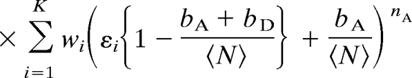
where p(n_A + n_D) is the probability of a bin containing n_A + n_D photons, b_A and b_D are the number of background counts per bin in the acceptor and donor channels, and 〈N〉 is the mean number of photons per bin (all of which can be obtained from experimental data).

For polyproline-20 in TFE, a three-species model was used (donor-only, all-trans, and C-terminal cis). The parameters w_i and ε_i were optimized by maximizing the joint likelihood of all observed bursts, where Eq. 1 gives the likelihood of the observation in an individual time bin. The efficiency histogram back-calculated from the optimal parameters is plotted in Fig. 3A. The largest fitted population in TFE has an efficiency of 0.34 and a population of 81% (excluding donor-only). The other species (apart from donor-only) has an efficiency of 0.53 and a population of 19%. These populations are close to the NMR values of 87.5 ± 3.0% for all-trans polyproline, and 12.5 ± 3.0% for molecules with a C-terminal cis proline. The corresponding efficiencies from simulation, determined by integrating I(t), are 0.40 and 0.61.

In water, the NMR data show that there is the possibility of many different polyproline conformations with various combinations of cis prolines (38 in total, neglecting the small population of molecules expected to have more than one internal cis proline), so any fit would be highly underdetermined. We therefore calculated the FRET efficiency histogram with the populations taken from the NMR analysis and the efficiencies calculated from the simulations for each of the 38 isomers, assuming a uniform distribution of internal cis residues. We find that the prediction of the histogram is in remarkably good agreement with the measured histogram.

Discussion

FRET has been extensively used for obtaining qualitative distance information in single-molecule experiments on biomolecules (14, 29, 30). More recently, experiments have suggested that despite the large chromophores and long linkers, it should be possible to obtain accurate quantitative distance information in both proteins and nucleic acids (15, 16, 19, 21, 31). However, quantitative analysis of single-molecule FRET experiments using polyproline of varying lengths as spacers between donor and acceptor dyes has raised some doubt. Using continuous wave excitation, Schuler et al. (15), and later Watkins et al. (21), found that the mean FRET efficiency was much higher than expected for polyproline acting as a rigid rod spacer and that the width of the FRET efficiency distribution is much greater than expected from shot noise alone. Schuler et al. (15) used molecular dynamics simulations of polyproline to attribute the high mean efficiency to flexibility of polyproline, assumed to be in the all-trans type II helix, whereas Watkins et al. (21) suggested that cis prolines would contribute to both the high efficiency and excess width, but did not carry out any structural analysis or molecular simulations. Our objective in this work has been to provide a more quantitative explanation of these two findings by repeating experiments on polyproline-20 using pulsed laser excitation and time-tagging of individual photons to obtain histograms of FRET efficiencies for single molecules and of time delays for subpopulations, NMR experiments to estimate both the location and fraction of cis prolines, and molecular dynamics simulations of polyproline that include cis residues, as well as the dyes and their flexible linkers. This information leads to a satisfactory quantitative explanation of both the high mean FRET efficiency and the excess width.

Our NMR experiments demonstrate that in water ≈30% of the molecules contain internal cis prolines, whereas in TFE there are no detectable internal cis prolines (Fig. 2); in both solvents, there is also a small population of cis proline at the C-terminal residue. The internal cis prolines produce kinks in the chain that bring the donor and acceptor dyes closer together, and immediately provide a qualitative explanation for both the higher mean efficiency and shorter lifetime in water compared with TFE and the greater width in excess of that expected from shot noise alone (Figs. 3 and 6). Can we explain these results quantitatively?

To do so, we carried out molecular dynamics simulations and developed a theoretical framework for analyzing FRET efficiency histograms. Distance distributions obtained from the simulations show that all-trans polyproline itself is relatively stiff, with rms fluctuations of 0.2 nm in end-to-end length (Fig. 5A). The much broader distribution of lengths (15) obtained in earlier simulations of polyproline with the same force field were a result of the integration step (2 fs) being too short for the friction (50 ps⁻¹) used (see SI Text). The persistence length for all-trans polyproline, calculated several different ways and with different force fields, is 9–13 nm (see Results and SI Fig. 10). This flexibility is too little to increase the FRET efficiency much above that expected for a rigid rod, even for the 40-residue polyproline in the study of Schuler et al. (15).

We have compared the results of the simulations with both the intensity and lifetime data (Fig. 6). In TFE there are only two populations of molecules: 88.5% all-trans and 12.5% with a cis residue at the C terminus. The result is that the fluorescence decay calculated from the simulations (see SI Text) differs only slightly from that expected for 100% all-trans polyproline. To calculate the fluorescence decay in water from the simulations, we used the fractions of C-terminal and internal cis residues from NMR and assumed an equal probability for a single cis residue at each internal position. This enumeration results in a total of 38 isomers. The internal cis residues have a much bigger effect than the C-terminal cis residues, and result in a large decrease in fluorescence lifetime compared with the all-trans molecule. The calculated fluorescence decay curves are in remarkably good accord with the observed histogram of donor time delays.

Calculation of FRET efficiency histograms requires careful consideration of both the shot noise and background fluorescence. We first ruled out any significant contribution to the width of the distribution from bleaching or blinking of the acceptor dye by comparing the FRET efficiency in the first and second half of each burst of photons, and by examining the distribution of continuous strings of donor photons (Fig. 4).

We calculated FRET efficiency histograms using a model that allows for multiple species with different FRET efficiency (see Eq. 1). In the case of TFE, maximum likelihood was used to determine optimal populations and efficiencies for the species, consistent with the distribution of donor and acceptor photons in the individual bursts as the molecules diffuse through the detection volume. The efficiency histogram computed from the optimal parameters explains the very small excess width above that expected from shot noise. The optimal populations are similar to those determined by NMR and the efficiencies are only slightly less than obtained from the simulations (Fig. 3). In the case of water, direct calculation of the efficiency histogram from 38 different isomers with populations determined from the NMR experiments and mean efficiencies from simulations is remarkably similar to the observed histogram. Although internal cis prolines bring the ends of the molecule closer together, the mean efficiency is only modestly increased because the dynamics associated with the additional flexibility is effectively slow relative to the donor lifetime (see SI Fig. 8).

We find that linker dynamics plays an important role: the donor dye is conjugated to the C-terminal cysteine residue by a very flexible five-carbon linker and undergoes large projected fluctuations (rms of 0.9 nm; Fig. 5B), compared with the much smaller fluctuations of the acceptor, attached to the C-terminal glycine by a two carbon linker (0.25 nm Fig. 5C). Thus, the overall donor-acceptor distance distribution in Fig. 5D largely reflects the mobility of the donor chromophore. Whereas this mobility has the advantage that the orientational contribution to FRET, κ², is close to the isotropic value of 2/3, it also means that the contribution of linker dynamics to donor-acceptor separation needs to be carefully considered when determining distance information from FRET.

A related question that arose in the course of this work was whether donor/acceptor dynamics might explain the discrepancy mentioned earlier concerning the R₀ in the classic study of Stryer and Haugland (1). We found that simulations that included the dynamics of a naphthyl donor and dansyl acceptor resulted in increased FRET efficiency, explaining a large part of the difference between the calculated curves using the experimentally determined R₀ and the fitted R₀ (see SI Fig. 11).

The consistency of the results from NMR, single-molecule lifetime and intensity measurements, and molecular dynamics simulations indicates that, despite the structural complexity, it is indeed possible to understand single-molecule FRET experiments with polyproline spacers in quantitative detail. These results, as well as the previous work on proteins unfolded by chemical denaturants (6–20), suggests that single-molecule FRET will become an increasingly powerful tool in investigations of structure distributions in protein folding and related problems.

Materials and Methods

NMR Spectroscopy.

¹H NOESY spectra were acquired for (Pro)₈Gly and (Pro)₂₀Gly in D₂O, and for (Pro)₂₀Gly in deuterated TFE (Cambridge Isotope Laboratoraties, Andover, MA) at 8°C to separate the water and H^α signals; similar results were obtained at 20°C. All spectra were acquired on an 800-MHz Bruker spectrometer.

Single-Molecule Instrument.

Single-molecule measurements were carried out with a Picoquant Microtime 200 confocal fluorescence microscope (Berlin, Germany). A 470-nm pulsed diode laser (20-MHz repetition rate, 80 ps FWHM, 35 μW average power) was used to excite the donor chromophore, and donor and acceptor fluorescence were detected by single-photon avalanche photodiodes. A TimeHarp200 card was used to record the detection channel (donor, acceptor), the absolute arrival time (100 ns resolution), and fluorescence lifetime (37 ps resolution) of each photon.

Molecular Dynamics Simulations.

Polyproline dynamics were investigated by using Langevin simulations of polyproline peptides of sequence Gly-(Pro)_n-Cys with the EEF1 implicit solvent force-field (32). The dye-linker dynamics were studied by using all-atom simulations (CHARMM27 force-field) of polyproline-dye fragments consisting of the peptide Gly-(Pro)₅-Cys linked either to a “donor” (attached to Cys using maleimide chemistry) or “acceptor” (attached to Gly by peptide chemistry) dyes. Simulations were run for 20 ns in explicit TIP3P water with periodic boundary conditions (4.67-nm box size) at constant pressure (1 atm) using NAMD (33). To calculate time-dependent transfer rates k_ET(t), composite trajectories were assembled from the three simulations by choosing random, independent time origins from each and evaluating k_ET(t) over the subsequent portions of the simulations (differences in units of time because of friction as described above were also accounted for). Further details of simulations and efficiency calculations are in SI Text

Note Added in Proof.

A recent study by Doose et al. (34) provides evidence for internal cis prolines in aqueous solutions from short-range (sub-nanometer) fluorescence quenching by photoinduced electron transfer in ensemble and FCS experiments on polyprolines up to 10 residues in length but does not quantify either the fraction of internal cis residues or their effect on the FRET efficiency.

References

- 1.Stryer L, Haugland RP. Proc Natl Acad Sci USA. 1967;58:719–726. doi: 10.1073/pnas.58.2.719. [DOI] [PMC free article] [PubMed] [Google Scholar]
- 2.Stryer L. Annu Rev Biochem. 1978;47:819–846. doi: 10.1146/annurev.bi.47.070178.004131. [DOI] [PubMed] [Google Scholar]
- 3.Cowan PM, McGavin S. Nature. 1955;176:501–503. doi: 10.1038/1761062a0. [DOI] [PubMed] [Google Scholar]
- 4.Schimmel PR, Flory PJ. Proc Natl Acad Sci USA. 1967;58:52–59. doi: 10.1073/pnas.58.1.52. [DOI] [PMC free article] [PubMed] [Google Scholar]
- 5.Ha T, Enderle T, Ogletree DF, Chemla DS, Selvin PR, Weiss S. Proc Natl Acad Sci USA. 1996;93:6264–6268. doi: 10.1073/pnas.93.13.6264. [DOI] [PMC free article] [PubMed] [Google Scholar]
- 6.Deniz AA, Dahan M, Grunwell JR, Ha TJ, Faulhaber AE, Chemla DS, Weiss S, Schultz PG. Proc Natl Acad Sci USA. 1999;96:3670–3675. doi: 10.1073/pnas.96.7.3670. [DOI] [PMC free article] [PubMed] [Google Scholar]
- 7.Jia YW, Talaga DS, Lau WL, Lu HSM, DeGrado WF, Hochstrasser RM. Chem Phys. 1999;247:69–83. [Google Scholar]
- 8.Deniz AA, Laurence TA, Beligere GS, Dahan M, Martin AB, Chemla DS, Dawson PE, Schultz PG, Weiss S. Proc Natl Acad Sci USA. 2000;97:5179–5184. doi: 10.1073/pnas.090104997. [DOI] [PMC free article] [PubMed] [Google Scholar]
- 9.Talaga DS, Lau WL, Roder H, Tang JY, Jia YW, DeGrado WF, Hochstrasser RM. Proc Natl Acad Sci USA. 2000;97:13021–13026. doi: 10.1073/pnas.97.24.13021. [DOI] [PMC free article] [PubMed] [Google Scholar]
- 10.Schuler B, Lipman EA, Eaton WA. Nature. 2002;419:743–747. doi: 10.1038/nature01060. [DOI] [PubMed] [Google Scholar]
- 11.Lipman EA, Schuler B, Bakajin O, Eaton WA. Science. 2003;301:1233–1235. doi: 10.1126/science.1085399. [DOI] [PubMed] [Google Scholar]
- 12.Rhoades E, Cohen M, Schuler B, Haran G. J Am Chem Soc. 2004;126:14686–14687. doi: 10.1021/ja046209k. [DOI] [PubMed] [Google Scholar]
- 13.Kuzmenkina EV, Heyes CD, Nienhaus GU. Proc Natl Acad Sci USA. 2005;102:15471–15476. doi: 10.1073/pnas.0507728102. [DOI] [PMC free article] [PubMed] [Google Scholar]
- 14.Schuler B. ChemPhysChem. 2005;6:1206–1220. doi: 10.1002/cphc.200400609. [DOI] [PubMed] [Google Scholar]
- 15.Schuler B, Lipman EA, Steinbach PJ, Kumke M, Eaton WA. Proc Natl Acad Sci USA. 2005;102:2754–2759. doi: 10.1073/pnas.0408164102. [DOI] [PMC free article] [PubMed] [Google Scholar]
- 16.Kuzmenkina EV, Heyes CD, Nienhaus GU. J Mol Biol. 2006;357:313–324. doi: 10.1016/j.jmb.2005.12.061. [DOI] [PubMed] [Google Scholar]
- 17.Sherman E, Haran G. Proc Natl Acad Sci USA. 2006;103:11539–11543. doi: 10.1073/pnas.0601395103. [DOI] [PMC free article] [PubMed] [Google Scholar]
- 18.Hoffmann A, Kane A, Nettels D, Hertzog DE, Baumgärtel P, Lengefeld J, Reichardt G, Horsley DA, Seckler R, Bakajin O, et al. Proc Natl Acad Sci USA. 2007;104:105–110. doi: 10.1073/pnas.0604353104. [DOI] [PMC free article] [PubMed] [Google Scholar]
- 19.Merchant KA, Best RB, Louis JM, Gopich IV, Eaton WA. Proc Natl Acad Sci USA. 2007;104:1528–1533. doi: 10.1073/pnas.0607097104. [DOI] [PMC free article] [PubMed] [Google Scholar]
- 20.Nettels D, Gopich IV, Hoffmann A, Schuler B. Proc Natl Acad Sci USA. 2007;104:2655–2660. doi: 10.1073/pnas.0611093104. [DOI] [PMC free article] [PubMed] [Google Scholar]
- 21.Watkins LP, Chang HY, Yang H. J Phys Chem A. 2006;110:5191–5203. doi: 10.1021/jp055886d. [DOI] [PubMed] [Google Scholar]
- 22.Clarke DS, Dechter JJ, Mandelkern L. Macromolecules. 1979;12:626–633. [Google Scholar]
- 23.Nir E, Michalet X, Hamadani KM, Laurence TA, Neuhauser D, Kovchegov Y, Weiss S. J Phys Chem B. 2006;110:22103–22124. doi: 10.1021/jp063483n. [DOI] [PMC free article] [PubMed] [Google Scholar]
- 24.Gopich I, Szabo A. J Chem Phys. 2005;122 doi: 10.1063/1.1812746. 014707-1-18. [DOI] [PubMed] [Google Scholar]
- 25.Gopich IV, Szabo A. J Phys Chem B. 2007;111:12925–12932. doi: 10.1021/jp075255e. [DOI] [PubMed] [Google Scholar]
- 26.Thirumalai D, Ha BY. Grosberg A. Theoretical and Mathematical Models in Polymer Research. New York: Academia; 1988. pp. 1–35. [Google Scholar]
- 27.Henry ER, Hochstrasser RM. Proc Natl Acad Sci USA. 1987;84:6142–6146. doi: 10.1073/pnas.84.17.6142. [DOI] [PMC free article] [PubMed] [Google Scholar]
- 28.Antonik M, Felekyan S, Gaiduk A, Seidel CAM. J Phys Chem B. 2006;110:6970–6978. doi: 10.1021/jp057257+. [DOI] [PubMed] [Google Scholar]
- 29.Kuhnemuth R, Seidel CAM. Single Mol. 2001;2:251–254. [Google Scholar]
- 30.Michalet X, Kapanidis AN, Laurence T, Pinaud F, Doose S, Pflughoefft M, Weiss S. Annu Rev Biophys Biomol Struct. 2003;32:161–182. doi: 10.1146/annurev.biophys.32.110601.142525. [DOI] [PubMed] [Google Scholar]
- 31.Lee NK, Kapanidis AN, Wang Y, Michalet X, Mukhopadhyay J, Ebright RH, Weiss S. Biophys J. 2005;88:2939–2953. doi: 10.1529/biophysj.104.054114. [DOI] [PMC free article] [PubMed] [Google Scholar]
- 32.Lazaridis T, Karplus M. Proteins. 1999;35:133–152. doi: 10.1002/(sici)1097-0134(19990501)35:2<133::aid-prot1>3.0.co;2-n. [DOI] [PubMed] [Google Scholar]
- 33.Phillips JC, Braun R, Wang W, Gumbart J, Tajkhorshid E, Villa E, Chipot C, Skeel RD, Kale L, Schulten K. J Comp Chem. 2005;26:1781–1802. doi: 10.1002/jcc.20289. [DOI] [PMC free article] [PubMed] [Google Scholar]
- 34.Doose S, Neuweiler H, Barsch H, Sauer M. Proc Natl Acad Sci USA. 2007;104:17400–17405. doi: 10.1073/pnas.0705605104. [DOI] [PMC free article] [PubMed] [Google Scholar]
Associated Data
This section collects any data citations, data availability statements, or supplementary materials included in this article.