

Abstract
In apo and holoCaM, almost half of the hydrogen bonds (H-bonds) at the protein backbone expected from the corresponding NMR or X-ray structures were not detected by h3 J NC′ couplings. The paucity of the h3 J NC′ couplings was considered in terms of dynamic features of these structures. We examined a set of seven proteins and found that protein-backbone H-bonds form two groups according to the h3 J NC′ couplings measured in solution. H-bonds that have h3 J NC′ couplings above the threshold of 0.2 Hz show distance/angle correlation among the H-bond geometrical parameters, and appear to be supported by the backbone dynamics in solution. The other H-bonds have no such correlation; they populate the water-exposed and flexible regions of proteins, including many of the CaM helices. The observed differentiation in a dynamical behavior of backbone H-bonds in apo and holoCaM appears to be related to protein functions.
Keywords: hydrogen bonding, proteins, calmodulin, h3JNC′ couplings
In a variety of small globular proteins, that is, crambin (Hee-chul et al. 2006), ubiquitin (Cordier and Grzesiek 1999), streptococcal protein G (Cornilescu et al. 1999), cold-shock protein A (Alexandrescu et al. 2001), parvalbumin, and intestinal fatty acid binding protein (Juranić et al. 2002), ∼80% of the hydrogen bonds (H-bonds) identified from application of geometrical criteria in the helices and sheets of the corresponding crystal structures have also been detected in solution via h3 J NC′ couplings. However, both NMR and IR spectroscopic studies have indicated the formation of solvent (water) H-bonds to the protein backbone (Juranić et al. 1996; Manas et al. 2000) that may weaken intraprotein H-bond networks (Juranić et al. 2003; Shenkarev et al. 2004; Wieczorek and Dannenberg 2005). Theoretical calculations predict a significant impact of protein solvation on the H-bond networks at the protein backbone (Dannenberg 2006). Increased dynamics of the protein backbone in solution (Karplus and McCammon 2002; Markwick et al. 2003) may also challenge the sustenance of H-bonds that appear in the proteins' crystal structures. A recent interpretation of the residual dipolar couplings (RDC) in streptococcal protein G invokes the possibility that correlated motions affect secondary-structure-determined H-bond networks (Bouvignies et al. 2005); structural flexibility may occur without much disruption of H-bonds. Such correlated motions are suggested to be rather slow, in the millisecond time regime, and may also be associated with a protein's function (Bouvignies et al. 2005).
To obtain further insight into how the solvent may affect the stability and dynamics of protein H-bond networks, we directed our studies to proteins that are known to have significant differences in backbone conformations in solution with respect to that observed in solids (Ikura and Ames 2006). Calmodulin (CaM) is one prominent example of this class of proteins. Calmodulin, which is involved in the regulation of many cellular systems (Cheung 1980; Falke et al. 1994; Carafoli and Klee 1999; Jurado et al. 1999; Nelson et al. 2002; Vetter and Leclerc 2003), undergoes significant conformational changes when it binds Ca2+ ions (Kuboniwa et al. 1995; Zhang et al. 1995a; Ikura 1996; Nelson and Chazin 1998; Evenas et al. 2001; Yang et al. 2002), or upon its interaction with various target proteins (Ikura et al. 1992; Meador et al. 1993, 1995; Vetter and Leclerc 2003). Structures of both calcium-free (apoCAM) and calcium-loaded (holoCAM) human calmodulin have been determined by X-ray crystal structure analysis (Chattopadhyaya et al. 1992; Schumacher et al. 2004) and by solution NMR spectroscopy (Kuboniwa et al. 1995; Zhang et al. 1995a; Chou et al. 2001), revealing differences between solid and solute structures. In holoCaM, differences are primarily in the backbone conformation of the linker connecting two globular domains; in apoCaM, several backbone H-bonds are intramolecular in solution but intermolecular in the crystal structure. Furthermore, exceptional structural plasticity can be seen in the CaM X-ray structures (Meador et al. 1993; Wilson and Brunger 2000), and several conformational substates were detected in solution (Slaughter et al. 2005). We, therefore, hypothesize that calmodulin may reveal differentiations in the dynamical behavior of the H-bonds under influence of solvent, and can depart greatly from the crystal structure H-bonds. We report here that the H-bond networks of apoCaM and holoCaM in solution, as detected by the h3 J NC′ couplings, support this premise.
Results
ApoCaM
The structure of human apoCaM in solution was determined long ago by use of NMR spectroscopy (Kuboniwa et al. 1995; Zhang et al. 1995a). The secondary structure in these apoCaM solution structures was identified primarily from NOE data on interproton distances (Fig. 1, top panel), that is, eight α-helices were identified from sequential NOE contacts. The secondary-structure assignments are also consistent with overall helical content as determined from circular dichroism data (Brzeska et al. 1983). Four α-helices were found in each of two globular lobes (N and C termini). The existence of these helices suggest that H-bonds should be detected by J coupling in both termini. Indeed, both X-ray (Schumacher et al. 2004) and NMR structures of apoCaM (Kuboniwa et al. 1995; Zhang et al. 1995a) are consistent in suggesting that α-helical h3 J NC′ couplings should be detected equally throughout both termini (Fig. 1, bottom three panels). However, this is not what we found when we measured the h3 J NC′ couplings of the backbone H-bonds in apoCaM (Fig. 1, second panel). Rather, we found that while the measured J couplings in the N terminus mainly agree with those predicted from the X-ray and solution structures, in the C terminus many H-bonds are not detected by J couplings. These results are consistent with an increased mobility and chemical exchange in the C-terminus lobe inferred from other NMR results (Tjandra et al. 1995). There is a particularly stark difference between the J couplings detected for helices E and H and those predicted from the structures.
Figure 1.

Sequential NOE distances of amide protons in apoCaM (Zhang et al. 1995a) (top, backbone h3 J NC′ couplings [second from top]) and relative sensitivity of J-HNCO experiment (third from top). (Central insert) The secondary structure of apoCaM; (rectangular boxes) helices; (arrows) the short β-sheet contacts. Detected β-sheet contacts are labeled with the corresponding residue numbers. (Three bottom inserts) Magnitudes of the h3 J NC′ calc couplings that we calculated for three of the reported structures (Kuboniwa et al. 1995; Zhang et al. 1995a) (in the 1QX5 structure [Schumacher et al. 2004], there are several intermolecular H-bonds [light-gray bars]).
The difference between the detected and expected H-bonds in the C terminus is not an artifact of the J-HNCO experiment sensitivity. Although in the C terminus (Fig. 1), the sensitivity of the experiment (mainly determined by 15N T2 relaxation) is lower; the detectability of the couplings is good even in the regions of lower sensitivity (i.e., helix F). In the instances of missing h3 J NC′ couplings (i.e., helix H), we still detected sequential 2 J NC′ and side-chain 3 J NC′ couplings that indicate a good detection threshold, estimated to be at 0.1–0.2 Hz. We estimate instead that low signal intensity prevented detection of eventual H-bonds for only seven residues (92, 100, 107, 131, 136, 139, 140).
The β-sheet contacts between the calcium-binding loops were detected by the h3 J NC′ couplings in positions 29 → 61, 63 → 27, and 102 → 134. In comparison with the X-ray and NMR structures (Fig. 1), H-bond couplings at positions 27 → 63, 100 → 136, and 136 → 100 are missing. Remarkable, in the C-terminus lobe where many H-bonds are not detected, a long H-bond chain is seen to extend over helix F and the β-sheet contact of the EF hand, (Fig. 2), connecting helix F with the Ca-IV-binding site.
Figure 2.
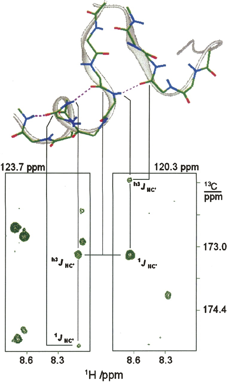
Strips from 3D HNCO-J spectrum displaying NC′ correlation peaks in the H-bond chain 107/108 → 104/105 → 101/102 → 102/134. The spectrum, recorded at the J-coupling evolution time of 1/4J = 32 msec, is the sum of two 3D HNCO-J spectra each collected for 4 d on a Bruker 600 MHz spectrometer equipped with a cryo-probe.
HoloCaM
The structure of human holoCaM in solution has been determined by the method of NMR residual dipolar couplings (Chou et al. 2001). That structure showed major differences from the X-ray crystal structure (Chattopadhyaya et al. 1992; Wilson and Brunger 2000) in that the long central helix connecting two lobes is split into two helices (D and E) with a short and flexible linker between them. Similar features were later observed in the X-ray structure of a “compact” CaM, induced by a minor post-translational modification (Fallon and Quiocho 2003). Excluding the region of the central linker, all these structures show similar H-bond networks. Therefore, corresponding h3 J NC′ couplings, calculated from the X-ray and the NMR structures, are comparable (Fig. 3) except in the region of the linker. However, in this work, the h3 J NC′ couplings of the backbone H-bonds we determined show that only a relatively low percentage of H-bonds are detected in the helices, especially in the N-terminus lobe (Fig. 3). Helix D of the N terminus has the fewest h3 J NC′ couplings, while helix G of the C terminus shows the greatest number of h3 J NC′ couplings. Again, we rule out sensitivity of the J-HNCO experiment as the reason for such a paucity of H-bond couplings; the overall sensitivity of the experiment is higher than from apoCaM and is almost equal for all helices (Fig. 3, top panel vs. Fig. 1, third panel).
Figure 3.

Relative sensitivity of J-HNCO experiment (top) and backbone h3 J NC′ couplings (second from top). (Central insert) The secondary structure of holoCaM; (rectangular boxes) helices; (arrows) the short β-sheet contacts. Detected β-sheet contacts are labeled with the corresponding residue numbers. (Bottom inserts) The magnitudes of the h3 J NC′ calc couplings that we calculated for two of the reported structures (Wilson and Brunger 2000; Chou et al. 2001).
The β-sheet contacts between the calcium-binding loops were detected by the h3 J NC′ couplings in positions 27 → 63, 63 → 27, 100 → 136, and 136 → 100, fully in agreement with the X-ray and NMR structures (Fig. 3).
Discussion
Protein backbone H-bonds detected by h3 J NC′ couplings in apo and holoCaM are all at the positions expected from the corresponding NMR or X-ray structures. Calculated h3 J NC′ couplings for these H-bonds have intensities, on average, that are comparable to the experimental values. However, almost half of the H-bonds that should be present were not detected. For most of these H-bonds, the h3 J NC′ couplings calculated from the respective H-bond geometries are well above a threshold level of detection achieved in this work (0.1–0.2 Hz). Since the integrity of the α-helical structure of two lobes of apo and holoCaM in solution has been amply proven by CD and NMR spectroscopy, the paucity of the h3 J NC′ couplings has to be considered within the dynamical features of these structures. As suggested in the introduction, we may have revealed a differentiation in the dynamical behavior of the H-bonds on a scale that is larger than has been observed in other proteins.
Protein backbone H-bonds that cannot be detected in solution by h3 J NC′ couplings, despite good evidence of overall structural integrity, have been noted before (Juranić et al. 2002; Assadi-Porter et al. 2003; Grzesiek et al. 2004). For example, protein reverse turns at position 4 ← 2 mostly do not show H-bond coupling (Juranić et al. 2002). For α-helices, considerable weakening of the h3 J NC′ couplings has been observed at solvent-exposed sides of helices (Juranić et al. 2003; Cordier and Grzesiek 2004; Shenkarev et al. 2004). The absence or weakening of the h3 J NC′ couplings was interpreted to be a consequence of water H-bonding to the backbone peptide groups (Juranić et al. 2003). Other interpretations suggest that a small bending of α-helices around a protein's hydrophobic core may weaken H-bonds at the solvent-exposed sides of the helices (Cordier and Grzesiek 2004). These interpretations do not preclude each other and have to be considered in conjunction with the H-bond dynamics in the solvent-exposed regions of proteins (Shenkarev et al. 2004). Thus, it has been suggested that correlated motions in the H-bond network of the protein backbone depend on “hydrophobic anchoring” of the protein side chains (Bouvignies et al. 2005). Solvent-exposed regions do not have such anchoring, and the backbone dynamics may not be as favorable for sustaining this H-bond network. For instance, helices E and H in holoCaM have tightly packed aromatic side chains that may serve as just such hydrophobic anchors (Fig. 4). In keeping with this inference, we have detected H-bond couplings only at positions closest to the anchored side chains. Reduced, or correlated, mobility due to the structural stabilization occasioned by these “anchorings” would maintain these H-bonds. The undetected H-bonds are, indeed, mainly on the side of helices that are expected to have exposure to solvent. Supporting information on the water exposure of the backbone carbonyl groups may be obtained from the size of the peptide–bond 1 J NC′ couplings (Fig. 4); couplings tend to be larger at the solvent-exposed side of helix (Juranić et al. 1996). This kind of information provides also a clue to the behavior of the E-helix in apoCaM, where almost all h3 J NC′ couplings are missing. As presented in Figure 4 (top), the 1 J NC′ couplings are indicative of even larger exposure of the E-helix to water in apoCaM.
Figure 4.

Hydrophobic contact of helices E and H in holoCaM. (Dashed lines) The H-bonds detected by h3 J NC′ couplings (magenta-colored region of the helices). (Top part) The peptide-bond 1 J NC′ couplings in the E-helix of apo and holoCAM.
Two (dynamical) subsets of H-bonds
By invoking specific types of peptide-group motions, one can rationalize the fact that α-helices that have good CD signals and sequential NOE contacts still may lack H-bonds with detectable J couplings. For instance, the correlated motions of peptide groups across H-bonds (Bouvignies et al. 2005) would maximally preserve h3 J NC′ couplings, while sequentially correlated motions of peptide groups (Pelupessy et al. 2003) may better preserve sequential NOE contacts.
Correlated motional modes of peptide groups across H-bonds were implied (Bouvignies et al. 2005) from the effect seen on several h3 J NC′ couplings in protein G. Such dynamics have not been directly observed, but, rather, they have been modeled from measured peptide-group orientations. If such correlated dynamics exist, the forces that govern them may influence the conformational state of the protein backbone in crystal structures. We therefore analyzed the crystal structures of seven proteins whose H-bond h3 J NC′ couplings in solution have been reported (crambin, ubiquitin, protein G, parvalbumin, and intestinal fatty acid binding protein) or are reported here (apoCaM and holoCaM). Backbone H-bonds seen in the crystal structures of these proteins may be divided into two subsets according to the magnitude of the h3 J NC′ couplings measured for the proteins in solution. The subset with |h3 J NC′| > 0.2 Hz shows correlations among the H-bond geometry parameters, while the other subset with |h3 J NC′| < 0.1 Hz (or h3 J NC′ not detected) shows no such correlation (Fig. 5). (We have left out a borderline group of H-bonds with 0.1 Hz < |h3 J NC′| < 0.2 Hz, which are close to the detection threshold, and their alliance to any of two groups may be influenced by experimental errors.) The main feature of the subset with |h3 J NC′| > 0.2 Hz (high-J subset in further text) is an angle/distance correlation of the H-bond parameters. Accordingly, at shorter H-bond distances, the deviation from the linearity at both donor (>N–H) and acceptor (O=C<) gets smaller (Fig. 5, top). Such correlation is consistent with the H-bond dipole–dipole attractive force (preference for short, linear H-bonds). It is also consistent with dynamical expansion–contraction of the H-bond network (less orientational pull at the larger distances). The angles at the acceptor end are proportionally larger by ∼30% in comparison to the donor angles, which agrees with there being a smaller orientation force of a weaker donor-dipole (>N–H). The actual attractive force is certainly more complex than dipole–dipole (Karplus and McCammon 2002; Morozov et al. 2004); an approximate fifth-order distance dependence of H-bond angles (Fig. 5, top) is indicative of quadrupol–quadrupol interaction. Irrespective of the exact nature of the forces governing the H-bond geometry of the high-J subset, the observed angle/distance constraints can cause correlated dynamics in solution.
Figure 5.

Angle–distance correlation of H-bonds from seven proteins (crambin, ubiquitin, protein G, parvalbumin, IFABP, and apo- and holo-calmodulin) divided into two subsets according to the magnitude of the H-bond couplings (|h3 J NC′| > 0.2 Hz, top; |h3 J NC′| < 0.1 Hz, bottom). The distance correlation for the donor angle, ΔαH (○), is matched with the correlation for the acceptor angle, ΔαO (□), upon scaling the latter by 0.72. (The full curved line) The fifth-power distance dependence (0.8d OH 5); (dashed lines) ∼90% containment boundaries. The peptide groups involved in the coordination to Ca2+ were excluded from the analysis.
The other, low-J subset, has many H-bonds with geometries that should give intense h3 J NC′ couplings, but the couplings are undetected in solution presumably because of unfavorable dynamics of the H-bonds. Evidently, if mobility is the only culprit, then the low-J subset of H-bonds does not persist in solution on the timescale of the h3 J NC′ couplings measurements (∼100 msec). It is unlikely that dynamical rupture of the H-bonds (Sheu et al. 2003) can exist on the timescale needed for disappearance of the J couplings, unless some other H-bonds are formed. A likely mechanism is one that involves bifurcated H-bonds of amide carbonyls with water (Juranić et al. 1996; Manas et al. 2000; Walsh et al. 2003; Shenkarev et al. 2004). Under dynamical conditions, the bifurcated H-bonds can fluctuate in the H-bond donor partner between water and amide proton with little structural stress to the α-helix (Shenkarev et al. 2004).
As an interesting aspect of the H-bond angle–distance correlation (Fig. 5), the low-J H-bonds can be predicted to some degree from crystal structures. The H-bonds with parameters outside of the angle–distance-correlation boundaries (dashed lines in Fig. 5) in solution have no detectable J couplings in 80% of the cases (90% for CaM). Prediction of the converse, namely, as to which H-bonds should have high-J couplings in solution, is less reliable. A probable cause for this is cooperativity within the H-bond networks. When low-J H-bonds are disrupted they may corrupt other neighboring H-bonds. For instance, the long central helix that exists in the holoCaM crystal structure breaks in solution between residues 76 and 82. From the crystal-structure H-bond geometries, we can predict three H-bonds—74 ← 78, 75 ← 79, and 77 ← 81—as undetectable by the J couplings, and these constitute half of the H-bonds in that region. Experimentally none are detected. Since the region is devoid of hydrophobic anchoring, the (predicted) weak H-bonds apparently corrupt the helical structure altogether.
The proposed dynamics of the low-J subset of H-bonds, which involve bifurcated H-bonds to water, should change the average orientation of the respective peptide groups. Such a hypothesis can be tested by analysis of RDCs of the peptide groups in solution. We tested this on holoCaM, for which both the high-resolution X-ray structure (Wilson and Brunger 2000) and solution RDCs (Chou et al. 2001) have been reported. As presented in Figure 6, the solution RDCs of peptide groups can be fitted well to the crystal structure for the high-J subset, while major deviations occur for the low-J subset.
Figure 6.

Experimental RDCs of peptide groups (Δ1 J HN, Δ1 J NC/0.12, and Δ1 J CCa/0.20) in α-helices of the holoCaM C terminus, in comparison with the calculated values for the corresponding crystal and solution structures. The crystal structure is represented by X-ray high-resolution structure 1exr-model-A (Wilson and Brunger 2000), while the solution structure is modeled from the X-ray structure to satisfy RDCs. The high-J and low-J data refer to the size of proton-donating H-bonds of the peptide groups. (Lower insert) The X-ray and the modeled solution structure of helix E. (Small arrows) Connection between peptide-group orientations and RDC fit for the peptide group in position 91/92. The hydrophobic anchoring residue is indicated.
To assess peptide-group orientations in solution, we have allowed changes of their orientations seen in the crystal structure until the solution RDCs were fitted. Notable changes in orientations occurred only for the peptide groups of the low-J subset. The majority of these peptide groups adopted orientations consistent with the higher exposure of carbonyl oxygen to water. We can now compare crystal and solution orientations of the peptide groups in helix E of holoCaM (Fig. 6), and verify the inferences we made from the analysis of the J couplings. Thus, we inferred the H-bonding of carbonyl oxygen to water at the exposed side of the helix. Indeed, the corresponding peptide groups are tilted into directions that should facilitate formation of such H-bonds.
Analogous analyses apply to the N terminus of holoCaM. The RDCs corresponding to the high-J subset can be fitted to the X-ray structure much better than those from the low-J subset. However, modeling of the peptide group orientations to fit RDCs proved less successful than in the C terminus. Such a result is consistent with much higher amplitudes of conformational mobility, which makes it impossible to account for the observed RDCs by a single model of peptide groups' average orientations without violating the chemical structure of the backbone.
If the proposed increased dynamics of the low-J subset of H-bonds is correct, one might expect there to be some correlation with the order parameter derived from 15N-relaxation measurements at the protein backbone, although the latter reflect only fast motions in the picosecond–nanosecond range. By comparing the occurrence of the low-J H-bonds with the reported order parameters in holoCaM (Barabato et al. 1992), it can be inferred that h3 J NC′ couplings are absent for order parameters below 0.6. This applies not only for the central helix, which breaks in solution (no H-bonds are therefore expected anyway), but also for some H-bonds that are part of α-helices that exist in solution (i.e., positions 14 ← 10, 114 ← 109, 147 ← 143). Among the high-J H-bonds, those with |h3 J NC′| > 0.7 Hz have order parameters above 0.7. These findings support the inference of a dynamic origin of H-bond differentiation in solution. However, the overall correlation between order parameters and H-bond couplings is weak, signifying that internal mobility on larger timescales (Ishima and Torchia 2003; Ishima et al. 2004) is likely more important for the couplings.
Significance of H-bonds in the low-J subset
Since most of the H-bonds in this subset are not detected directly, their existence in proteins in solution has to be inferred from other experimental evidence on the protein secondary structure. Not all H-bonds from the solid proteins necessarily survive in solution, thus existence of each H-bond of the low-J type has to be considered carefully. Yet, regions of protein secondary structure populated by these H-bonds may have significance for protein function. As indicated in the introduction, small, globular, single-domain proteins that have been studied so far have <20% H-bonds in the low-J subset. In apo and holoCaM, whose functionality requires conformational changes, the population of the low-J subset scales up to ∼50%. Also, the intraprotein distribution of the low-J subset appears to shift into regions slated for an initial ligand-induced conformational change. For instance, in apoCaM (Fig. 7), the C-terminus helices have H-bonds mostly from the low-J subset (in contrast to the N-terminus helices), and Ca2+ binding starts first in the C terminus (Malmendal et al. 1999). Upon calcium binding, in the reconstructed C terminus of holoCaM, the low-J subset of H-bonds decreases below 50%. In contrast, calcium binding to the N terminus increases the population of the low-J subset in this domain from 50% to ∼70%. Such a result for holoCaM agrees with multiconformational refinement of its X-ray structure (Wilson and Brunger 2000), which showed higher conformational plasticity in the N terminus. These results may imply greater adaptability of the N terminus in the function of holoCaM. Indeed, when binding to target peptides, the changes of affinity to calcium are more pronounced in the N terminus (Peersen et al. 1997). The peptide-binding ability of holoCaM primarily depends on the exposed hydrophobic patches, formed from the residues of several helices upon calcium binding (Zhang et al. 1995a). It is not surprising that helix D in the N terminus, which contributes most to the creation of these water-exposed hydrophobic patches, is also the least populated with the J-detected H-bonds (Fig. 7).
Figure 7.

Comparison of the high-J subset H-bonds in apoCaM (top) and holoCaM (bottom). The population of the helices with the detected H-bonds is represented by the shades of the rectangular boxes: (black) >70%; (gray) ∼50%; (empty) <30%. Detected β-sheet contacts are labeled with the corresponding residue numbers.
Conclusion
Protein-backbone H-bonds that are identified from geometrical criteria in solid or solution structures of proteins form two broad groups defined by the h3 J NC′ couplings measured in solutions by NMR spectroscopy. The H-bonds detected directly in solution by the h3 J NC′ couplings (at threshold >0.2 Hz) show correlation among the H-bond geometrical parameters in solid proteins, and appear supported by the protein dynamics in solution.
The H-bonds not directly detected in solution by the h3 J NC′ couplings (or have values <0.2 Hz) populate more flexible and water-exposed regions of the protein secondary structure. Calmodulin, whose function requires large conformational changes, is especially populated by such H-bonds. It appears that distribution of such H-bonds within apo and holoCaM indicates regions of the protein structure that have higher flexibility related to protein function.
The flexibility, or conformational mobility, addressed by the J-profile of H-bonds should be useful for understanding dynamical heterogeneity within the regular secondary-structure motifs of proteins. In conjunction with data on the angular distribution of peptide group orientations, it furthers our understanding of the correlated dynamics within H-bond networks of proteins.
Material and Methods
Calmodulin (CaM) expression, enrichment, and purification
Human calmodulin cDNA was subcloned into a pET-15b expression vector (Novagen) using standard cloning techniques. No purification tag was introduced into the construct. The identity of the insert was confirmed by Big Dye dideoxy terminator cycle sequencing using vector-specific as well as gene-specific oligonucleotide primers. CaM was overexpressed in the BL21(DE3)-pLysS strain of Escherichia coli (Single Shot; Novagen). Uniform 13C,15N enrichment was achieved by growing cells in Luria-Bertani medium and then inducing in minimal media containing 13C-glucose and 15NH4Cl, following established protocols (Marley et al. 2001). Isotopically labeled and unlabeled CaM was purified using a slight modification to an existing procedure (Putkey et al. 1985): 5 mM CaCl2 was added to the cleared cell lysate, which was loaded onto a phenyl-Sepharose CL-4B column (Sigma), and the CaM was eluted with 1 mM EGTA. CaM fractions were further purified using a HiTrap Q column (Amersham Biosciences) and a 0–1 M NaCl gradient. CaM was >95% pure, judging by SDS-gel electrophoresis and Coomassie Brilliant Blue staining. The identity of the CaM was confirmed by N-terminal sequencing as well as by LS-MS analysis of the tryptic digests of labeled and unlabeled CaM. The molecular weight and labeling efficiency (96%) were verified by ESI-MS by direct infusion.
NMR measurements
The 2.0 mM sample of uniformly 15N,13C-labeled apoCaM (quartz tube) was prepared in 20 mM HEPES (pH 7.5), 100 mM KCl, 1 mM EDTA, and 1 mM EGTA. The 2.0 mM sample of uniformly 15N,13C-labeled holoCaM was prepared in the same buffer as for apoCaM, with addition of 20 mM Ca2+. In both samples, 5% D2O was added. The H-bond h3 J NC′ and others' nJ NC′ coupling constants were measured (Bruker Avance 600 MHz spectrometer equipped with a cryogenic probe) using a constant time 3D J-HNCO experiment (Cordier and Grzesiek 1999; Cornilescu et al. 1999). The nJ NC′ coupling constants were determined by fitting the time evolution of all observed NC′ couplings for a particular peptide-group nitrogen as described in an earlier publication (Juranić and Macura 2001). For the constant time of ∼32 msec, J-HNCO spectra were recorded for seven evolution times (16 msec, 20 msec, 24 msec, 28 msec, 31 msec, 32 msec, 33 msec), with four times increased numbers of scans (64) for the evolution times in bold (1 J NC′ couplings quenched). Experimental errors of the coupling constants were estimated from the quality of fitting data at all evolution times.
Parameters describing H-bond geometry
The angles, dihedral angles, and distances defining the geometry of the H-bonds were calculated from protein structures in the PDB—apoCaM: 1QX5 (Schumacher et al. 2004), 1CFD (Kuboniwa et al. 1995), 1DMO (Zhang et al. 1995b), holoCaM: 1EXR (Wilson and Brunger 2000), 1J70 and 1J7P (Chou et al. 2001), crambin: 1EJG (Jelsch et al. 2000), protein G: 1IGD (Derrick and Wigley 1994), ubiquitin: 1UBQ (Vijay-Kumar et al. 1987), parvalbumin: 4CPV (Kumar et al. 1990), and IFABP: 1IFC (Sacchettini 1989). For structures lacking amide protons, H-bond distances were calculated after protons were added to their respective PDB structures by software (CHARM22), and the NH distance was set to the value observed in the ultra-high-resolution X-ray structure (Jelsch et al. 2000) of crambin (1.01 Å). The geometrical criteria for H-bonds were set to H···O distances <2.5 Å, and bond angles at the donor and acceptor <90°. The magnitudes of the h3 J NC′ couplings, expected on the basis of H-bond geometry, were calculated using the Barfield-type formula (Barfield 2002). We used the first term of Equation 13 from the original Barfield paper (Barfield 2002), which has been parameterized against experimental data from protein G. In α-helices, the first term gives practically the same values as the whole Equation 13. The complete Equation 13 is expected to give better estimates for β-sheet H-bonds. However, the few β-sheet H-bonds in CaM were calculated to be closer to experimental values using the first term only. Therefore, we preferred using a simple form of the first term of Equation 13, that is, it can be written as h3 J NC′ = −cos2θ exp[−3.2(r HO − 1.68)].
Fitting of peptide-group dipolar couplings
Calculations of RDCs from the model structures and fitting to the experimental values were done using our own programs written in MATLAB. The main routines of the program are:grid search for protein orientation; grid search for individual peptide group orientations and positions (in selected protein orientation); fitting of calculated to experimental RDCs by SVD; validation of protein-backbone structure parameters (bond distances, angles, dihedrals); and validation of H-bond geometry against the experimental h3 J NC′ couplings.
In the SVD fitting, the molecular alignment tensor and rhombicity was treated as an invariant. We used alignment tensors and rhombicities of CaM termini determined in the original RDC work (Chou et al. 2001), that is, D a(NH) = 10.8 Hz, R = 0.42 for the N terminus; and D a(NH) = −9.6 Hz, R = 0.64 for the C terminus. The initial orientation of CaM domains (1exr.pdb structure) was determined by fitting the high-J-coupling RDCs only. Then the low-J RDCs were fitted (grid search) by allowing discrete changes in the orientation of peptide planes. For each tested orientation of a peptide group, the protein backbone was relaxed (by grid search of peptide group translations) to fulfill chemical structure constraints, or it was rejected. In the final refinements, protein orientation and peptide-plane orientations and positions were adjusted for best fitting of RDCs from both the low-J and high-J sets. We did not constrain geometries to H-bonds of the regular α-helix but rather constrained geometries to comply with the experimental h3 J NC′ couplings. This is a significant departure from earlier RDC optimization of the CaM solution structure (Chou et al. 2001). The H-bond geometry was constrained to the experimental h3 J NC′ ± 0.3 Hz via the Barfield equation (Equation 13, first term). Experimental NOE distances were not used as constraints. However, the final structures of the helices all have sequential HN–HN distances within 0.5 Å of the corresponding ones found in X-ray (1exr.pdb) or NMR structures (1j7o.pdb). Such differences generally cannot be addressed by comparison with experimental NOEs in proteins.
The reported multiconformer models of the X-ray crystal structure (1exr.pdb) (Wilson and Brunger 2000) were tested separately and also in their combinations for the best fit to the experimental RDCs. For the CaM C terminus, the best choice was model A, and in the N terminus, model B.
Electronic supplemental material
The Electronic supplemental material contains tables of h3 J NC′ couplings in apo and holo calmodulin, and a table of atomic coordinates for the RDC optimized structure of the C-terminus backbone.
Footnotes
Supplemental material: see www.proteinscience.org
Reprint requests to: Nenad Juranić, Mayo Foundation, 200 First Street SW, Rochester, MN 55905, USA; e-mail: juranic.nenad@mayo.edu; fax: (507) 284-8433.
Article published online ahead of print. Article and publication date are at http://www.proteinscience.org/cgi/doi/10.1110/ps.062689807.
References
- Alexandrescu A.T., Snyder, D.R., and Abildgaard, F. 2001. NMR of hydrogen bonding in cold-shock protein A and an analysis of the influence of crystallographic resolution on comparisons of hydrogen bond lengths. Protein Sci. 10: 1856–1868. [DOI] [PMC free article] [PubMed] [Google Scholar]
- Assadi-Porter F.M., Abildgaard, F., Blad, H., and Markley, J.L. 2003. Correlation of the sweetness of variants of the protein brazzein with patterns of hydrogen bonds detected by NMR spectroscopy. J. Biol. Chem. 278: 31331–31339. [DOI] [PubMed] [Google Scholar]
- Barabato G., Ikura, M., Kay, L.E., Pastor, R.W., and Bax, A. 1992. Backbone dynamics of calmodulin studied by 15N relaxation using inverse detected two-dimensional NMR spectroscopy: The central helix is flexible. Biochemistry 31: 5269–5278. [DOI] [PubMed] [Google Scholar]
- Barfield M. 2002. Structural dependencies of interresidue scalar coupling h3 J NC, and donor 1H chemical shifts in the hydrogen bonding regions of proteins. J. Am. Chem. Soc. 124: 4158–4168. [DOI] [PubMed] [Google Scholar]
- Bouvignies G., Bernado, P., Meier, S., Cho, K., Grzesiek, S., Bruschweiler, R., and Blackledge, M. 2005. Identification of slow correlated motions in proteins using residual dipolar and hydrogen-bond scalar couplings. Proc. Natl. Acad. Sci. 102: 13885–13890. [DOI] [PMC free article] [PubMed] [Google Scholar]
- Brzeska H., Venyaminov, S.Vu., Grabarek, Z., and Drabikowski, W. 1983. Comparative studies on thermostability of calmodulin, skeletal muscle troponin C and their fragments. FEBS Lett. 153: 169–173. [DOI] [PubMed] [Google Scholar]
- Carafoli E. and Klee, C. 1999. Calcium as cellular regulator. Oxford University Press, New York.
- Chattopadhyaya R., Meador, W.E., Means, A.R., and Quiocho, F.A. 1992. Calmodulin structure refined at 1.7 angstrom resolution. J. Mol. Biol. 228: 1177–1192. [DOI] [PubMed] [Google Scholar]
- Cheung W.Y. 1980. Calmodulin plays a pivotal role in cellular regulation. Science 207: 19–27. [DOI] [PubMed] [Google Scholar]
- Chou J.J., Li, S.P., Klee, C.B., and Bax, A. 2001. Solution structure of Ca2+-calmodulin reveals flexible hand-like properties of its domains. Nat. Struct. Biol. 8: 990–997. [DOI] [PubMed] [Google Scholar]
- Cordier E. and Grzesiek, S. 1999. Direct observation of hydrogen bonds in proteins by interresidue 3h J NC′ scalar couplings. J. Am. Chem. Soc. 121: 1601–1602. [DOI] [PubMed] [Google Scholar]
- Cordier F. and Grzesiek, S. 2004. Quantitative comparison of the hydrogen bond network of A-state and native ubiquitin by hydrogen bond scalar couplings. Biochemistry 43: 11295–11301. [DOI] [PubMed] [Google Scholar]
- Cornilescu G., Hu, J.S., and Bax, A. 1999. Identification of the hydrogen bonding network in a protein by scalar couplings. J. Am. Chem. Soc. 121: 2949–2950. [Google Scholar]
- Dannenberg J.J. 2006. The importance of cooperative interactions and a solid-state paradigm to proteins: What peptide chemists can learn from molecular crystals. Adv. Protein Chem. 72: 227. [DOI] [PubMed] [Google Scholar]
- Derrick J.P. and Wigley, D.B. 1994. The 3rd igg-binding domain from streptococcal protein-G—An analysis by X-ray crystallography of the structure alone and in a complex with Fab. J. Mol. Biol. 243: 906–918. [DOI] [PubMed] [Google Scholar]
- Evenas J., Malmendal, A., and Akke, M. 2001. Dynamics of the transition between open and closed conformations in a calmodulin C-terminal domain mutant. Structure 9: 185–195. [DOI] [PubMed] [Google Scholar]
- Falke J.J., Drake, S.K., Hazard, A.L., and Peersen, O.B. 1994. Molecular tuning of ion-binding to calcium signaling proteins. Q. Rev. Biophys. 27: 219–290. [DOI] [PubMed] [Google Scholar]
- Fallon J.L. and Quiocho, F.A. 2003. A closed compact structure of native Ca2+-calmodulin. Structure 11: 1303–1307. [DOI] [PubMed] [Google Scholar]
- Grzesiek S., Cordier, F., Jaravine, V., and Barfielfd, M. 2004. Insight into biomolecular hydrogen bonds from hydrogen bond scalar couplings. Prog. Nucl. Magn. Reson. Spectrosc. 45: 275–300. [Google Scholar]
- Hee-chul A., Juranić, N., Macura, S., and Markley, J.L. 2006. Three-dimensional structure of the water-insoluble protein crambin in dodecylphosphocholine micelles and its minimal solvent-exposed surface. J. Am. Chem. Soc. 128: 4398–4404. [DOI] [PMC free article] [PubMed] [Google Scholar]
- Ikura M. 1996. Calcium binding and conformational response in EF-hand proteins. Trends Biochem. Sci. 21: 14–17. [PubMed] [Google Scholar]
- Ikura M. and Ames, J.B. 2006. Genetic polymorphism and protein conformational plasticity in the calmodulin superfamily: Two ways to promote multifunctionality. Proc. Natl. Acad. Sci. 103: 1159–1164. [DOI] [PMC free article] [PubMed] [Google Scholar]
- Ikura M., Clore, G.M., Gronenborn, A.M., Zhu, G., Klee, C., and Bax, A. 1992. Solution structure of calmodulin-target peptide complex by multidimensional NMR. Science 256: 632–638. [DOI] [PubMed] [Google Scholar]
- Ishima R. and Torchia, D.A. 2003. Extending the range of amide proton relaxation dispersion experiments in proteins using a constant-time relaxation-compensated CPMG approach. J. Biomol. NMR 25: 243–248. [DOI] [PubMed] [Google Scholar]
- Ishima R., Baber, J., Louis, J.M., and Torchia, D.A. 2004. Carbonyl carbon transverse relaxation dispersion measurements and ms-μs timescale motion in a protein hydrogen bond network. J. Biomol. NMR 29: 187–198. [DOI] [PubMed] [Google Scholar]
- Jelsch C., Teeter, M.M., Lamzin, V., Pichon-Pesme, V., Blessing, R.H., and Lecomte, C. 2000. Accurate protein crystallography at ultra-high resolution: Valence electron distribution in crambin. Proc. Natl. Acad. Sci. 97: 3171–3176. [DOI] [PMC free article] [PubMed] [Google Scholar]
- Jurado L.A., Chockalingam, P.S., and Jarrett, H.W. 1999. Apocalmodulin. Physiol. Rev. 79: 661–682. [DOI] [PubMed] [Google Scholar]
- Juranić N. and Macura, S. 2001. Correlations among 1 J NC′ and h3 J NC′ coupling constants in the hydrogen-bonding network of human ubiquitin. J. Am. Chem. Soc. 123: 4099–4100. [DOI] [PubMed] [Google Scholar]
- Juranić N., Likic, V.A., Prendergast, F.G., and Macura, S. 1996. Protein–solvent hydrogen bonding studied by NMR 1 J NC′ coupling constant determination and molecular dynamics simulations. J. Am. Chem. Soc. 118: 7859–7860. [Google Scholar]
- Juranić N., Moncrieffe, M.C., Likic, V.A., Prendergast, F.G., and Macura, S. 2002. Structural dependencies of h3 J NC′ scalar coupling in protein H-bond chains. J. Am. Chem. Soc. 124: 14221–14226. [DOI] [PubMed] [Google Scholar]
- Juranić N., Macura, S., and Prendergast, F.G. 2003. H-bonding mediates polarization of peptide groups in folded proteins. Protein Sci. 12: 2633–2636. [DOI] [PMC free article] [PubMed] [Google Scholar]
- Karplus M. and McCammon, J.A. 2002. Molecular dynamics simulations of biomolecules. Nat. Struct. Biol. 9: 646–652 Erratum. [DOI] [PubMed] [Google Scholar]
- Kuboniwa H., Tjandra, N., Grzesiek, S., Ren, H., Klee, C.B., and Bax, A. 1995. Solution structure of calcium-free calmodulin. Nat. Struct. Biol. 2: 768–776. [DOI] [PubMed] [Google Scholar]
- Kumar V.D., Lee, L., and Edwards, B.F. 1990. Refined crystal structure of calcium-liganded carp parvalbumin 4.25 at 1.5-Å resolution. Biochemistry 29: 1404–1412. [DOI] [PubMed] [Google Scholar]
- Malmendal A., Evenas, J., Forsen, S., and Akke, M. 1999. Structural dynamics in the C-terminal domain of calmodulin at low calcium levels. J. Mol. Biol. 293: 883–899. [DOI] [PubMed] [Google Scholar]
- Manas E.S., Getahun, Z., Wright, W.W., DeGrado, W.F., and Vanderkooi, J.M. 2000. Infrared spectra of amide groups in α-helical proteins: Evidence for hydrogen bonding between helices and water. J. Am. Chem. Soc. 122: 9883–9890. [Google Scholar]
- Markwick P.R., Sprangers, R., and Sattler, M. 2003. Dynamic effects on J-couplings across hydrogen bonds in proteins. J. Am. Chem. Soc. 125: 644–645 Erratum. [DOI] [PubMed] [Google Scholar]
- Marley J., Lu, M., and Bracken, C. 2001. A method for efficient isotopic labeling of recombinant proteins. J. Biomol. NMR 20: 71–75. [DOI] [PubMed] [Google Scholar]
- Meador W.E., Means, A.R., and Quiocho, F.A. 1993. Modulation of calmodulin plasticity in molecular recognition on the basis of X-ray structures. Science 262: 1718–1721. [DOI] [PubMed] [Google Scholar]
- Meador W.E., George, S.E., Means, A.R., and Quiocho, F.A. 1995. X-ray-analysis reveals conformational adaptation of the linker in functional calmodulin mutants. Nat. Struct. Biol. 2: 943–945. [DOI] [PubMed] [Google Scholar]
- Morozov A.V., Kortemme, T., Tsemekhman, K., and Baker, D. 2004. Close agreement between the orientation dependence of hydrogen bonds observed in protein structures and quantum mechanical calculations. Proc. Natl. Acad. Sci. 101: 6946–6951. [DOI] [PMC free article] [PubMed] [Google Scholar]
- Nelson M.R. and Chazin, W.J. 1998. An interaction-based analysis of calcium-induced conformational changes in Ca2+ sensor proteins. Protein Sci. 7: 270–282. [DOI] [PMC free article] [PubMed] [Google Scholar]
- Nelson M.R., Thulin, E., Fagan, P.A., Forsen, S., and Chazin, W.J. 2002. The EF-hand domain: A globally cooperative structural unit. Protein Sci. 11: 198–205. [DOI] [PMC free article] [PubMed] [Google Scholar]
- Peersen O.B., Madsen, T.S., and Falke, J.J. 1997. Intermolecular tuning of calmodulin by target peptides and proteins: Differential effects on Ca2+ binding and implications for kinase activation. Protein Sci. 6: 794–807. [DOI] [PMC free article] [PubMed] [Google Scholar]
- Pelupessy P., Ravindranathan, S., and Bodenhausen, G. 2003. Correlated motions of successive amide N-H bonds in proteins. J. Biomol. NMR 25: 265–280. [DOI] [PubMed] [Google Scholar]
- Putkey J.A., Slaughter, G.R., and Means, A.R. 1985. Bacterial expression and characterization of proteins derived from the chicken calmodulin cDNA and calmodulin processed gene. J. Biol. Chem. 260: 4704–4712. [PubMed] [Google Scholar]
- Sacchettini J.C., Gordon, J.I., and Banaszak, L.J. 1989. Refined apoprotein structure of rat intestinal fatty acid binding protein produced in Escherichia coli . Proc. Natl. Acad. Sci. 86: 7736–7740. [DOI] [PMC free article] [PubMed] [Google Scholar]
- Schumacher M.A., Crum, M., and Miller, M.C. 2004. Crystal structures of apocalmodulin and an apocalmodulin/SK potassium channel gating domain complex. Structure 12: 849–860. [DOI] [PubMed] [Google Scholar]
- Shenkarev Z.O., Balashova, T.A., Yakimenko, Z.A., Ovchinnikova, T.V., and Arseniev, A.S. 2004. Peptaibol zervamicin IIB structure and dynamics refinement from transhydrogen bond J couplings. Biophys. J. 86: 3687–3699. [DOI] [PMC free article] [PubMed] [Google Scholar]
- Sheu S.Y., Yang, D.Y., Selzle, H.L., and Schlag, E.W. 2003. Energetics of hydrogen bonds in peptides. Proc. Natl. Acad. Sci. 100: 12683–12687. [DOI] [PMC free article] [PubMed] [Google Scholar]
- Slaughter B.D., Unruh, J.R., Allen, M.W., Urbauer, R.J.B., and Johnson, C.K. 2005. Conformational substates of calmodulin revealed by single-pair fluorescence resonance energy transfer: Influence of solution conditions and oxidative modification. Biochemistry 44: 3694–3707. [DOI] [PubMed] [Google Scholar]
- Tjandra N., Kuboniwa, H., Ren, H., and Bax, A. 1995. Rotational-dynamics of calcium-free calmodulin studied by 15N-NMR relaxation measurements. Eur. J. Biochem. 230: 1014–1024. [DOI] [PubMed] [Google Scholar]
- Vetter S.W. and Leclerc, E. 2003. Novel aspects of calmodulin target recognition and activation. Eur. J. Biochem. 270: 404–414. [DOI] [PubMed] [Google Scholar]
- Vijay-Kumar S., Bugg, C.E., and Cook, W.J. 1987. Structure of ubiquitin refined at 1.8 Å resolution. J. Mol. Biol. 194: 531–544. [DOI] [PubMed] [Google Scholar]
- Walsh S.T., Cheng, R.P., Wright, W.W., Alonso, D.O., Daggett, V., Vanderkooi, J.M., and DeGrado, W.F. 2003. The hydration of amides in helices; a comprehensive picture from molecular dynamics, IR, and NMR. Protein Sci. 12: 520–531 Erratum. [DOI] [PMC free article] [PubMed] [Google Scholar]
- Wieczorek R. and Dannenberg, J.J. 2005. Enthalpies of hydrogen-bonds in α-helical peptides. An ONIOM DFT/AM1 study. J. Am. Chem. Soc. 127: 14534–14535. [DOI] [PubMed] [Google Scholar]
- Wilson M.A. and Brunger, A.T. 2000. The 1.0 angstrom crystal structure of Ca2+-bound calmodulin: An analysis of disorder and implications for functionally relevant plasticity. J. Mol. Biol. 301: 1237–1256. [DOI] [PubMed] [Google Scholar]
- Yang W., Lee, H.W., Hellinga, H., and Yang, J.J. 2002. Structural analysis, identification, and design of calcium-binding sites in proteins. Protein Struct. Funct. Genet. 47: 344–356. [DOI] [PubMed] [Google Scholar]
- Zhang M., Tanaka, T., and Ikura, M. 1995a. Calcium-induced conformational transition revealed by the solution structure of apo calmodulin. Nat. Struct. Biol. 2: 758–767. [DOI] [PubMed] [Google Scholar]
- Zhang M.J., Tanaka, T., Farrow, N.A., Kay, L.E., and Ikura, M. 1995b. Multidimensional NMR-studies of the structure and dynamics of calcium-free calmodulin. Protein Eng. 8: 30. [Google Scholar]