

Abstract
A sample of 35 independent molecular dynamics (MD) simulations of calmodulin (CaM) equilibrium dynamics was prepared from different but equally plausible initial conditions (20 simulations of the wild-type protein and 15 simulations of the D129N mutant). CaM’s radius of gyration and backbone mean-square fluctuations were analyzed for the effect of the D129N mutation, and simulations were compared with experiments. Statistical tests were employed for quantitative comparisons at the desired error level. The computational model predicted statistically significant compaction of CaM relative to the crystal structure, consistent with the results of small-angle X-ray scattering (SAXS) experiments. This effect was not observed in several previously reported studies of (Ca2+)4-CaM, which relied on a single MD run. In contrast to radius of gyration, backbone mean-square fluctuations showed a distinctly non-normal and positively skewed distribution for nearly all residues. Furthermore, the D129N mutation affected the backbone dynamics in a complex manner and reduced the mobility of Glu123, Met124, Ile125, Arg126, and Glu127 located in the adjacent α-helix G. The implications of these observations for the comparisons of MD simulations with experiments are discussed. The proposed approach may be useful in studies of protein equilibrium dynamics where MD simulations fall short of properly sampling the conformational space, and when the comparison with experiments is affected by the reproducibility of the computational model.
Keywords: MD simulations, protein dynamics, precision, reproducibility, accuracy, calmodulin
Protein conformational flexibility is ubiquitous and is necessary for protein function (Debrunner and Frauenfelder 1982; Zàvodszky et al. 1998; Zaccai 2000). At physiological temperatures, protein motions are extraordinarily complex, with characteristic times spanning >10 orders of magnitude. Protein conformational dynamics are governed by the laws of classical physics, and the description of forces involved in protein dynamics through empirical force-fields leads to molecular dynamics (MD) computer simulations (McCammon and Harvey 1987; Brooks et al. 1988). MD simulations are the principal theoretical method for studies of protein dynamics, routinely used to provide insight into microscopic dynamics of proteins and to complement experiments (Karplus and McCammon 2002).
The utility of protein MD simulations rests on our ability to compare the predictions of such simulations with experiments. If the predictions regarding some properties of interest are in agreement with the experiments, we may hypothesize that other dynamic properties, in particular ones that may not be readily accessible experimentally, are also correctly predicted by the computational model. This may provide new insights into the system of interest and may lead to novel hypotheses and, ultimately, to the testing of the hypothesis with new experiments. Central to driving this cycle of knowledge is the ability to quantitatively compare MD simulations with experiments. The comparison of MD simulations carried out under different conditions is also very important, in particular for the advancement of the simulation methodology (i.e., comparison of simulations based on different force-fields) or for comparative studies of similar systems (the effect of a point mutation for example).
When repeated from slightly different but equally plausible initial conditions, MD simulations of protein equilibrium dynamics predict different values for the same dynamic property of interest (Elofsson and Nilsson 1993; Auffinger et al. 1995; Likić and Prendergast 2001). These variations occur because MD simulations fall short of properly sampling a protein’s conformational space, an effect known as the “sampling problem” (Straub et al. 1994; Auffinger et al. 1995; Caves et al. 1998; Hess 2002). In 1995, when 1-nsec MD simulations of fully solvated proteins were hardly attainable, Clarage and coworkers (1995) speculated that the sampling problem may be alleviated with a simulation time of 100 nsec. More recently, several 40-nsec MD simulations of HPr and T4-lysozyme were analyzed for convergence in sampling (Hess 2002). Not only did these simulations fail to provide a complete picture of the protein’s conformational space, they also suggested that this goal will remain unattainable in the foreseeable future (Hess 2002).
The central question concerning the reproducibility of MD simulations can be restated as follows: How do we know that some property observed in an MD simulation, which may lend itself to some important biological or physical interpretation, is not merely an “accident” of the particular simulation? For example, in two 4-nsec MD simulations, one of Ca2+-loaded and one of Ca2+-free calmodulin (CaM), it was observed that the central helix remained straight in the Ca2+-loaded simulation but was bent in the Ca2+-free simulation (Komeiji et al. 2002). The investigators suggested that this indicated an allosteric change in CaM conformation induced by Ca2+ ions. In another, unrelated study, 15 independent 1-nsec MD simulations of Ca2+-loaded CaM were performed (Likić et al. 2003). In these simulations, the central helix remained straight in some MD runs but was bent in others, suggesting that bending of the central helix in any single simulation is a random event, occurring with a certain probability given the simulation time. While bending of the CaM central helix may well be influenced by the bound Ca2+ ions, it seems unwarranted to draw such a conclusion based on only two observations, i.e., one Ca2+-free and one Ca2+-loaded simulation.
The above example would suggest that predictions derived from protein MD simulations behave as a sample drawn from a certain parent population. Thus, to understand predictions of MD simulations in quantitative terms, one needs to understand the central tendency (such as the population mean) and the variability (such as the population standard deviation) of the parent population from which the predictions are “drawn.” It follows that given some dynamic property of interest, understanding of the parent distribution of the prediction is of central importance for quantitative comparison of simulations with experiments. By using this approach, we analyzed 35 independent MD simulations of fully solvated Ca2+-loaded wild-type CaM and its D129N mutant.
CaM is a small protein of 148 amino acid residues (Fig. 1 ▶) that acts as a principal modulator of intracellular Ca2+ signaling pathways (Crivici and Ikura 1995; Berridge et al. 1998). CaM shows an extreme conformational plasticity in target recognition, which is believed to be associated with the conformational flexibility and its “unusual” dynamic properties (Meador et al. 1993; Weinstein and Mehler 1994; Crivici and Ikura 1995). We demonstrate the application of the hypothesis testing to the analysis of two different dynamic properties routinely calculated from protein MD simulations: radius of gyration (Rg; a typical global property) and backbone mean-square (MS) fluctuations (a typical local property of the polypeptide chain). In terms of the observed probability distributions, Rg and MS fluctuations provide two extremes that we anticipate will be encountered in the analysis of other dynamic properties. We show that regardless of the nature of the MD property of interest, statistical methods provide a powerful approach for quantitative comparison of MD simulations with experiments. The results are contrasted with previous MD simulations of CaM, and the implications of the proposed approach are discussed in the wider context of protein MD simulations.
Figure 1.

Schematic diagram of the CaM crystal structure (Babu et al. 1988) used as the initial structure in all MD simulations. Bound Ca2+ ions are shown as filled spheres, and four Ca2+ binding sites are labeled I, II, III, and IV. The α-helix G, adjacent to the mutation site D129N, which is the first residue in the Ca2+-binding loop, is labeled. Molecular graphics created with Molscript (Kraulis 1991).
Results
Radius of gyration
Rg is defined as the square root of the moment of inertia per unit mass: Rg = (I/M)1/2, where M = ∑mi is the total protein mass and I = ∑miri2 is the moment of inertia. In these equations, the summation is over all atoms, and ri is the distance of the ith atom from the protein’s center of mass. Thus Rg is related to the global shape of the protein molecule; i.e., Rg is a measure of the spatial spread of the protein mass.
Small-angle X-ray scattering (SAXS) studies (Heidorn and Trewhella 1988; Matsushima et al. 1989; Kataoka et al. 1991a,b) suggested that in solution CaM adopts a more compact conformation compared with the extended dumbbell structure observed in several independently solved crystal structures (Babu et al. 1988; Taylor et al. 1991; Chattopadhyaya et al. 1992). In this work we address the following three topics: (1) whether our computational model predicts that the single mutation D129N has an effect on the Rg; (2) whether the Rg predicted by MD simulations is in agreement with the extended dumbbell structure observed in the crystal state (specifically, the structure that was used to provide initial coordinates for MD simulations) (Babu et al. 1988); and (3) whether the Rg predicted by MD simulations is in agreement with the Rg determined by SAXS (Heidorn and Trewhella 1988; Matsushima et al. 1989; Kataoka et al. 1991a,b).
The Rg calculated from our MD simulations is shown in Figure 2 ▶. A single value of Rg was obtained as an average over a single MD simulation, and therefore, our data set consisted of 35 data points spanning multiple simulations: 20 obtained from wild type–CaM simulation (wt simulation set), and 15 obtained from D129N–CaM simulations (m1 simulation set). To assess which statistical tests can be applied, we first addressed the question of whether the data originated from a normal parent distribution. Although some deviations from the straight line in the quantile versus quantile plot were observed for the wt data set (Fig. 3 ▶), a more formal Shapiro-Wilk test for normality (Madansky 1988) showed no significant evidence to reject the normal distribution assumption (wt data set, P-value = 0.3; m1 data set, P-value > 0.9).
Figure 2.

Boxplot of the radius of gyration calculated from the three simulation sets: wt (wild-type CaM, 20 data points), m1 (CaM D129N mutant, 15 data points), and wt + m1 (combined wild-type and CaM D129N mutant simulations, a total of 35 data points). The horizontal dash-dot line at 22.0 Å represents the radius of gyration calculated from the crystal structure of CaM (Babu et al. 1988), which was used as the initial structure in all MD simulations.
Figure 3.
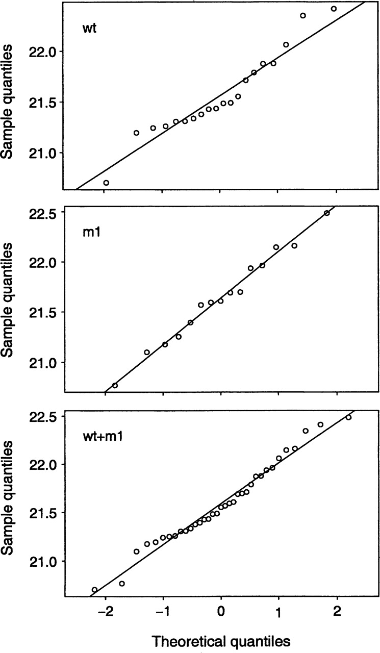
Normal probability plots (quantile vs. quantile plot) for the three data sets: wt (wild-type CaM, 20 data points), m1 (CaM D129N mutant, 15 data points), and wt + m1 (combined wild-type and CaM D129N mutant simulations, a total of 35 data points). The straight line is plotted through the upper and lower quartiles to help assess the linearity of the relationship.
Since no evidence against the hypothesis of normality was found, we used the classical t-test to assess the hypothesis that the samples wt and m1 originated from the parent populations with equal means. The F-test for the equality of variances (Lyman and Longnecker 2001) provided no evidence against the hypothesis that the variances of the two data sets are equal (P-value = 0.6), and the two-sample t-test provided no evidence against the equal means hypothesis (P-value = 0.6). This is also the first statistical test that provides us with a physical insight: the Rg as predicted from wild-type (wt) and D129N CaM simulations (m1) statistically cannot be distinguished. In other words, our computational model predicts that a single, conservative mutation within one lobe of CaM does not have a pronounced effect on the CaM’s Rg.
Because we cannot distinguish the data sets wt and m1 in terms of means, variances, and normality, we combined them into a single data set (wt + m1) for the purpose of comparison with the experimental data. This in effect amounts to neglecting the effect of the mutation D129N on the Rg. The combined data set (wt + m1) thus contained 35 values calculated from independent MD simulations.
The Rg calculated from the crystal structure of CaM (Babu et al. 1988), which was used as the initial structure in MD simulations, is 22.0 Å. To compare this to results of MD simulations, we tested the null hypothesis that the parent population of the data set wt + m1 had the mean of 22.0 Å; based on the t-test , we can reject this hypothesis (P-value of 3 × 10⁻⁶). Thus our MD simulations predict that in solution CaM adopts a more compact conformation compared with the fully elongated conformation observed in the crystal structure, which was used to initialize these simulations.
A number of Rg values of Ca2+-saturated CaM determined from SAXS measurements are shown in Table 1. Assuming that the uncertainties given by the investigators represent experimental uncertainties in the mean of the parent population, we can test these values against the population parameters estimated from MD simulations. The results show a considerable agreement between the 1-nsec computational model and SAXS experiments (Table 1).
Table 1.
t-Test comparison of MD simulation with CaM radius of gyration determined in X-ray structural studies (crystal state) and small-angle X-ray scattering studies (solution state)
| Method | Rg (Å) | Agreement with MD simulations |
| X-ray structure | ||
| Babu et al. 1988a | 22.0 | No (P = 3.4 × 10⁻⁶) |
| Small-angle X-ray scattering studies | ||
| Heidorn and Trewhella 1988 | ||
| Moore | 21.3 ± 0.2 | Yes (P = 0.21) |
| Guinier | 21.0 ± 0.6 | Yes (contains Smean)b |
| Matsushima et al. 1989 | ||
| Guinier | 21.5 ± 0.3 | Yes (contains Smean)b |
| Kataoka et al. 1991a | ||
| Moore | 22.0 ± 0.1 | No (P = 1.4 × 10⁻⁴) |
| Guinier | 21.4 ± 0.1 | Yes (P = 0.21) |
“Moore” and “Guinier” refer to two alternative analyses of the small-angle X-ray scattering data (see the corresponding references for details).
a The crystal structure used to provide the initial CaM coordinates in MD simulations reported here.
b The reported value contains the sample mean (Smean = 21.59 Å).
Backbone MS fluctuations
MS fluctuations are routinely determined from temperature (Debye-Waller) factors in the context of protein X-ray structure determination (Petsko and Ringe 1984), and are often calculated from MD trajectories (Karplus and McCammon 1983; Elofsson and Nilsson 1993; Clarage et al. 1995). Twenty wild-type CaM simulations (wt set) and 15 D129N-CaM simulations (m1 set) were processed to result in 35 independent sample points for each residue (backbone MS fluctuations were calculated for each residue as the average over N, Cα, C′ atoms).
The high degree of independence of the two CaM domains is well established experimentally. The two CaM lobes (Fig. 1 ▶) reorient nearly independently in solution (Barbato et al. 1992), and N- and C-terminal domain fragments retain their Ca2+-binding properties and structural response to Ca2+ binding, as observed in intact CaM (Evenäs et al. 1999, 2001). Since the mutation D129N is located in the Ca2+ binding loop IV of the C-terminal domain, we expect that the mutation D129N has little or no effect on the internal dynamics of the N-terminal lobe. To assess this hypothesis, we compared the backbone MS fluctuations observed in the simulation sets wt and m1.
Preliminary inspection of the distribution of calculated MS fluctuations showed that the sample distributions are distinctly non-normal. A typical histogram of calculated MS fluctuations is shown in Figure 4 ▶, which shows specifically MS fluctuations predicted for Ser17. Similar sample distributions were observed for other residues in both the N-terminal and the C-terminal domain of CaM. We used the Wilcoxon rank sum test (Lyman and Longnecker 2001) to compare the probability distributions of the parent populations for a given residue. In this case the null hypothesis was that the parent populations that give rise to samples observed in wt and m1 simulations are identical. No evidence against this hypothesis was found for the N-terminal domain of CaM when wt and m1 simulations were compared. At the significance level of 0.02, only two residues (Leu4 and Gly61) appeared to have different probability distributions of the parent populations. This is a rather weak evidence given that 70 residues were considered (residues 5–74) and that both Leu4 and Gly61 deviations occurred in isolation, involving only a single residue, which is not expected if the dynamic properties of the polypeptide chain were indeed affected. Thus, we conclude that the computational model predicted that the dynamics of the N-terminal domain are not affected by the mutation D129N, which is both close to the intuitive picture and consistent with the experimental evidence.
Figure 4.

The histogram of backbone mean-square fluctuations for Ser17 calculated from combined wt + m1 simulations (a total of 35 data points). Ser17 is located in the N-terminal lobe of CaM, which is not expected to be affected by the D129N mutation (located in the C-terminal lobe). This was confirmed by the Wilcoxon rank sum test, which provided no evidence against the hypothesis that backbone mean-square fluctuations for the N-terminal lobe residues predicted from the two sets of simulations were drawn from the same parent probability distribution. The situation was different for the C-terminal lobe (see Fig. 6 ▶).
The absence of detectable statistical differences between the two sets wt and m1 for the N-terminal domain of CaM justifies merging them into a single data set, which then provides an increased sample size. The MS fluctuations for the N-terminal domain of CaM predicted by MD simulations and those derived from temperature (Debye-Waller) factors reported in the crystal structure are shown in Figure 5 ▶. A close qualitative agreement between predicted and measured MS fluctuations is apparent. However, the boxplot of MS fluctuations calculated from MD simulations also shows that (1) the parent probability distribution is positively skewed for nearly all residues, and (2) the nature of the parent probability distribution varies and depends on the residue position within the polypeptide chain. Both points suggest a complex behavior and imply that any sound quantitative comparison of predicted and experimental MS fluctuations must take into account non-normal properties of the parent probability distribution in predicted MS fluctuations.
Figure 5.

Boxplot of calculated backbone mean-square fluctuations for the N-terminal lobe of CaM (residues 5–74) for the combined wt + m1 MD simulation set. The mean-square fluctuations derived from temperature (Debye-Waller) factors reported in the crystal structure used to initiate all MD simulations are shown in solid line (no correction for lattice disorder was applied). The backbone mean-square fluctuations predicted from MD simulations show a close qualitative agreement with the experimental data. However, the sample distributions of backbone mean-square fluctuations predicted from MD simulations imply non-normal parent probability distributions, highly dependent on the identity and the position of individual residues within the polypeptide chain.
The MS fluctuations in the C-terminal domain showed a significantly different picture. The Wilcoxon rank sum test applied on the residues of the C-terminal domain (residues 78–147) implied differences in the probability distribution of the parent populations for one isolated internal residue (Thr117) and two terminal residues (Met145 and Thr146) at the significance level of 0.02. This situation is similar to the deviations of Leu4 and Gly61 observed in the N-terminal domain. In addition, five contiguous residues (Glu123, Met124, Ile125, Arg126, and Glu127) were observed to have altered parent probability distributions in the D129N mutant compared with the wild-type CaM (Fig. 6 ▶). These residues are located in the C-terminal domain of α-helix G, immediately adjacent to the mutation site (Asp129). Figure 7 ▶ shows boxplots of MS fluctuations calculated for residues Glu123, Met124, Ile125, Arg126, and Glu127. It is apparent that the mutation D129N lowered the backbone MS fluctuations of Glu123, Met124, Ile125, Arg126, and Glu127, thus reducing the backbone mobility in the adjacent α-helix G.
Figure 6.

Wilcoxon rank sum test for the residues in the C-terminal lobe comparing backbone mean-square fluctuations between the wild-type (wt) and D129N mutant (m1) simulations. The mutation D129N affected the mean-square fluctuations of five residues located in the C-terminal half of α-helix G, which is immediately adjacent to the mutation site Asp129. The residues whose dynamics were affected are not symmetrically distributed around the mutation site; notably, the mutation did not affect the 12 residues involved in the Ca2+ binding loop between α-helices G and H, including Asn129, which is the first residue in this loop (see Fig. 7 ▶). The positions of the four α-helices (E, F, G, and H) located in the C-terminal lobe of CaM are shown, together with their interhelical loops and bound Ca2+ ions (small circles).
Figure 7.
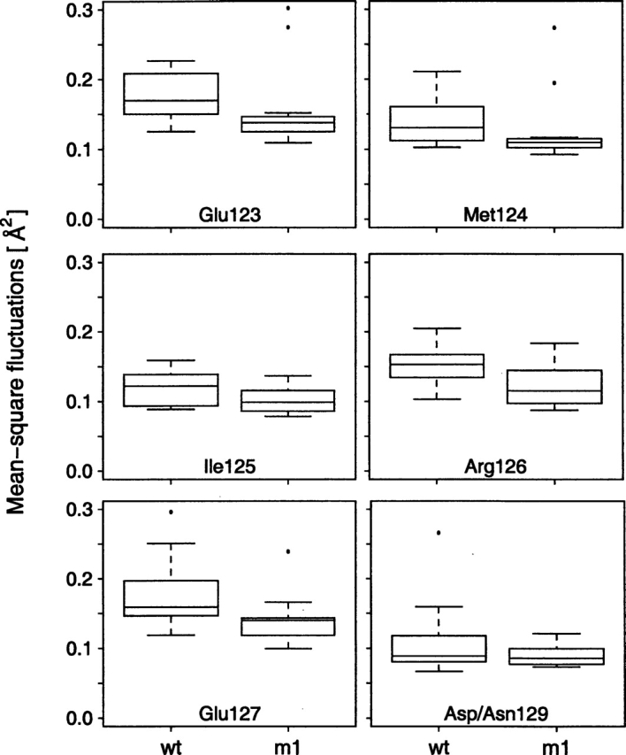
Boxplot of calculated mean square fluctuations for residues Glu123, Met124, Ile125, Arg126, and Glu127 for wild-type (wt) and D129N mutant (m1) simulations. These residues failed the Wilcoxon rank sum test under the null hypothesis that the samples wt and m1 were drawn from the same parent probability distribution (P-values shown in Fig. 6 ▶). The observed sample distribution did not provide such evidence for the backbone mean-square fluctuations at the site of mutation, the residue Asp/Asn129 (P = 0.5, the boxplot also shown).
Discussion
A sample of 35 independent MD simulations of fully solvated (Ca2+)4-CaM and its mutant D129N was presented. We demonstrate that such a sample can be analyzed by statistical hypothesis testing to support or refute some preconceived hypothesis about the observed variable(s) at the desired error level. MD simulations implied a compaction of (Ca2+)4-CaM relative to the crystal structure (Table 1), consistent with the results of SAXS experiments (Heidorn and Trewhella 1988; Matsushima et al. 1989; Kataoka et al. 1991a). This compaction has not been observed in several previously reported MD studies of (Ca2+)4-CaM, which employed a similar computational model in terms of both methodology and the force-field but relied on a single MD simulation (Wriggers et al. 1998; Yang et al. 2001; Komeiji et al. 2002). However, when random variation is taken into account, previously reported MD simulations of (Ca2+)4-CaM are consistent with our results.
The analysis of the predicted Rg provided no evidence against the hypothesis that the sample was generated by a normal parent probability distribution. The situation was quite different for MS fluctuations, which showed a distinctly non-normal and positively skewed distribution for nearly all residues (probably well approximated by the gamma family with two parameters: scale, shape). Therefore, to assess the effect of the D129N mutation on the CaM dynamics, we used a nonparametric test to compare calculated MS fluctuations in wild-type and D129N-mutant simulations. The Wilcoxon rank sum test was applied to N-terminal and C-terminal domain residues, and for the sake of simplicity, each residue was treated independently. On physical grounds, we expect that dynamics of residues adjacent in the sequence or residues proximal in the three-dimensional structure are not independent. The simple Bonferroni P-value adjustment could be applied; however, this would amount to a scaling of P-values and therefore would not alter the overall picture shown in Figure 6 ▶. We are currently investigating more advanced corrections that would take into account both sequence and spatial dependency of residues in the polypeptide chain.
The mutation D129N, located in Ca2+ binding loop IV of the C-terminal domain, affects a monodendate ligand to the Ca2+ ion [in position 1(X) of the 12-residue EF-hand Ca2+ binding loop]. Aspartate in this position is invariant in all known EF-hands (Strynadka and James 1989). The mutation Asp → Asn in the analogous EF-hand of troponin C disrupted Ca2+ binding and resulted in a functionally inactive protein (Babu et al. 1992). In our MD simulations, the mutation D129N exerted a complex effect on the backbone MS fluctuations (Fig. 6 ▶). The observed MS fluctuations of Glu123, Met124, Ile125, Arg126, and Glu127 were lower in the D129N mutant, suggesting that the mutation stiffened the adjacent α-helix G (Fig. 7 ▶). The shape of the parent probability distribution could provide additional insights into this effect. However, >15–20 sample points are required to obtain an accurate shape of the parent probability distribution, especially in a distinctly non-normal case as observed here.
The traditional approach in MD simulations of protein equilibrium dynamics is to perform a single (or a very few), but as long as possible, MD simulation. There are several important advantages inherent in the approach presented here. First, the results are reproducible to the extent that can be estimated a priori from the size of the collected sample (i.e., the number of independent MD runs), Second, the larger the number of independent MD runs, the greater is the reproducibility of results and also the power of subsequent statistical analysis (i.e., the ability to discern increasingly smaller effects). For example, a sufficiently large sample may be able to discern the effect of the D129N mutation on the CaM Rg.
An inherent feature of the proposed approach is that the total simulation time must be considered explicitly to be a part of the computational model, together with the employed force-field, water model, and the structure used to initialize the simulations. At first glance this may appear as a drawback because, in principle, properties arising from protein equilibrium dynamics should not depend on time. However, because in MD simulations a protein’s conformational space is not completely sampled, the results actually do depend on the simulations time. For example, in recently reported MD simulations of bacterial outer membrane protein FhuA, atomic MS fluctuations predicted from MD simulations increased steadily when calculated for the simulation times ranging from 0.5–8 nsec (Feraldo-Gómez et al. 2003). Therefore, in MD simulations of protein equilibrium dynamics, the total simulation time should be considered a part of the computational model unless, of course, it can be demonstrated that the property of interest does not depend on the simulation time.
MD simulations are stochastic in nature, and therefore, very infrequent, so-called “rare events” may be observed in any single MD run. In the context of multiple MD simulations, the term “rare event” refers to any process observed infrequently in only one MD run or a very few MD runs within the collected sample. The probability of such a process cannot be predicted reliably, no matter how large the sample is. Furthermore, a rare event may result in values that are outside of the likely range (i.e., outliers), which in turn may skew the overall picture obtained from the sample of MD runs. Therefore, it is highly desirable to detect such events early in the analysis. In principle, this could be done by finding outliers in data; however, finding outliers in a sample drawn from an unknown probability distribution is a nontrivial task. Our preliminary results suggest that analogs of the z-score based on outlier resistant estimators such as median absolute deviation perform well. This point merits further investigation; however, it is clear that a sample of MD simulations provides a much better opportunity to deal with rare events compared with the situation when only one (or a few) MD runs are collected.
The drawback of the proposed approach is the amount of work involved. In the sample of 35 independent MD simulations, each simulation was independently prepared, run, and analyzed upon completion. Subsequently, results were pooled together to give the global view of the sample. Thus the human work involved exceeds many times the work required to run and analyze one long MD simulation (e.g., a single 35-nsec MD run). However, this is in part because the tools for automation are lacking. Furthermore, running many simulations initialized from different initial conditions is well suited for distributed computing (Rhee et al. 2004). The distributed computing approach has the potential to provide a multitude of independent MD runs and thousands of sample points for any property of interest, thereby allowing one to deduce fine features of the parent probability distribution even in the case when the departures from normality are significant. Therefore, far more detailed comparisons of MD simulations, with experiments employing the methods described here, will be possible in the near future.
Materials and methods
A total of 35 MD simulations 1 nsec each were completed, 20 of the wild-type CaM (wt simulation set) and 15 of the D129N mutant (m1 simulation set). For each MD simulation, a unique initial configuration was prepared in such a way to provide a slightly different, but equally plausible, representation of the system under study (see below).
All MD simulations were carried out with the program NAMD2 (versions 22 and 23b2) (Åquist et al. 1986) and the CHARMM 22 force-field (MacKerell et al. 1998). Periodic boundary conditions and the particle-mesh Ewald method for the treatment of long-range electrostatic interactions were employed (Schlick et al. 1999). An integration step of 1 fsec was used to propagate equations of motion in the microcanonical ensemble (NVE). Nonbonded van der Waals interactions were smoothly truncated at 12.0 Å, with the switching function activated at 10.0 Å. Water molecules were represented with the TIP3P water model, as described previously (Likić et al. 2003). We used the parameters for the calcium ion obtained from the study of another EF-hand protein, calbindin (Marchand and Roux 1998). In all MD simulations, the X-ray structure of mammalian Ca2+-saturated CaM refined at 2.2 Å (Protein Data Bank code 3CLN) was used as the initial structure (Babu et al. 1988). Four Ca2+ ions and 69 ordered water oxygen sites observed in the crystal structure were also included in the initial structure. Five residues missing in the crystal structure (residues 1–4 and residue 148) were reconstructed in an extended conformation. All charged residues were taken in their standard states at pH 7, which resulted in a total protein charge of −16 for wild-type CaM, and −15 for the mutant D129N.
The simulated unit cell was a rectangular parallelepiped, with dimensions 89 × 67 × 67 Å or 90 × 78 × 78 Å, depending on the simulation set (see Table 2). In MD simulations wt-a and m1, 28 Na+ ions and 13 Cl− ions were added to neutralize the system and to mimic the solution with an ionic strength of ~100 mM. In simulations from the set wt-b, 40 Na+ ions and 24 Cl− ions were added to the system to create similar ionic conditions.
Table 2.
An overview of MD simulations from the sets wt-a, wt-b, and m1.
| Simulation set | No. of 1 nsec simulations | Protein | Box size (Å) |
| wt-a | 15 | wt-CaM | 89 × 67 × 67 |
| wt-b | 5 | wt-CaM | 90 × 78 × 78 |
| m1 | 15 | D129N-CaM | 89 × 67 × 67 |
In all simulations, the initial structure was the X-ray structure of mammalian Ca2+-saturated CaM refined at 2.2 Å (Protein Data Bank code 3CLN) (Babu et al. 1988).
wt-CaM is the wild-type CaM; D129N is the Asp129 → Asn CaM mutant.
To prepare initial configurations, two boxes of pure water were created by randomly positioning the appropriate number of water molecules within 89 × 67 × 67 Å and 90 × 78 × 78 Å rectangular parallelepipeds. After the initial minimization and equilibration, the simulations of pure water were run for 1 nsec (89 × 67 × 67 Å box) and 300 psec (90 × 78 × 78 Å box). The coordinates were saved every 100 psec, resulting in 10 (89 × 67 × 67 Å box) and three (90 × 78 × 78 Å box) equilibrated water configurations. These water configurations were combined with the protein crystal structure to create initial configurations for protein MD simulations. For each protein simulation, the water box was chosen randomly (89 × 67 × 67 Å box for wt-a and m1 simulations, and 89 × 67 × 67 Å box for wt-b simulations). The CaM crystal structure, including Ca2+ ions and 69 crystal structure water molecules, was placed within the box, centered and oriented with respect to the protein, and overlapping water molecules were deleted to create the initial configuration for a protein simulation. The cutoff for the selection of overlapping water molecules was chosen from the range 2.3–2.5 Å. The purpose of this was to create a unique initial solvent configuration for each protein simulation, and care was taken that no two simulations used both the same equilibrated water box and the water deletion cutoff.
The total number of atoms was ~40,000 in simulations wt-a and m1 and ~55,000 in simulations from the set wt-b. Each protein MD simulation was equilibrated for 390 psec prior to running 1 nsec of production dynamics, except for a single simulation from the m1 set, which was equilibrated for 300 psec. For each protein simulation, 1 nsec of equilibrium dynamics was represented with a trajectory containing 1000 coordinate frames spaced at 1 psec.
The individual globular domains of CaM remained structurally stable in all simulations, close to the crystal structure conformation. For both domains (N-terminal and C-terminal), the average RMS deviations versus the initial crystal structure were typical for MD simulations of globular proteins, as shown in Table 3. Throughout all MD runs, the four Ca2+ ions remained in their EF-hand binding sites. The simulations were completed at an average temperature of ~298 K (Table 3). A detailed analysis of the solvation and dynamics of Ca2+-binding sites in D129N-CaM simulations was presented previously (Likić et al. 2003).
Table 3.
Minimum/maximum average RMS deviations and average temperatures for the simulation sets wt-a, wt-b, and m1
| Simulation set | N-terminal average RMSDa (min/max, Å) | C-terminal average RMSDb (min/max, Å) | Average temperature (min/max, K) |
| wt-a | 1.16/2.46 | 1.09/2.28 | 298.2/298.4 |
| wt-b | 1.38/2.00 | 1.19/1.39 | 298.0/298.2 |
| m1 | 1.29/2.52 | 1.00/1.36 | 297.1/299.4 |
The average RMS deviation and temperature was evaluated as time average for each MD simulation, and “min/max” refers to the minimum/maximum time average observed within the simulation set.
a Backbone RMS deviations of the N-terminal domain (residues 5–74) vs. the crystal structure that was used to initialize simulations.
b Backbone RMS deviations of the C-terminal domain (residues 78–147) vs. the crystal structure that was used to initialize simulations.
Backbone MS fluctuations
Atomic MS fluctuations were calculated in a standard way, by aligning Cα atoms to remove the overall translation and rotation of the protein, with the first coordinate frame of dynamics in each simulation used as a reference. The backbone MS fluctuations were calculated from MD simulation by averaging positional fluctuations for N, Cα, and C′ atoms for each residue.
Acknowledgments
This work was supported in part by the Peter Doherty Fellowship from the Australian NHMRC (V.A.L.) and by NIH grant GM28835 (E.E.S.).
Article and publication are at http://www.proteinscience.org/cgi/doi/10.1110/ps.051681605.
References
- Åquist, J., Sandblom, P., Jones, T.A., Newcomer, M.E., van Gunsteren, W.F., and Tapia, O. 1986. Molecular dynamics simulations of the holo and apo forms of retinol binding protein. J. Mol. Biol. 192 593–604. [DOI] [PubMed] [Google Scholar]
- Auffinger, P., Louise-May, S., and Westhof, E. 1995. Multiple molecular dynamics simulations of the anticodon loop of tRNAAsp in aqueous solution with counterions. J. Am. Chem. Soc. 117 6720–6726. [Google Scholar]
- Babu, Y.S., Bugg, C.E., and Cook, W.J. 1988. Structure of calmodulin refined at 2.2 Å resolution. J. Mol. Biol. 204 191–204. [DOI] [PubMed] [Google Scholar]
- Babu, A., Su, H., Ryu, Y., and Gulati, J. 1992. Determination of residue specificity in the EF-hand of troponin C for Ca2+ coordination, by genetic engineering. J. Biol. Chem. 267 15469–15474. [PubMed] [Google Scholar]
- Barbato, G., Ikura, M., Kay, L.E., Pastor, R.W., and Bax, A. 1992. Backbone dynamics of calmodulin studied by 15N relaxation using inverse detected two-dimensional NMR spectroscopy: The central helix is flexible. Biochemistry 31 5269–5278. [DOI] [PubMed] [Google Scholar]
- Berridge, M.J., Bootman, M.D., and Lipp, P. 1998. Calcium: A life and death signal. Nature 395 645–648. [DOI] [PubMed] [Google Scholar]
- Brooks III, C.L., Karplus, M., and Pettitt, B.M. 1988. Proteins: A theoretical perspective of dynamics, structure and thermodynamics. John Wiley, New York.
- Caves, L.S.D., Evanseck, J.D., and Karplus, M. 1998. Locally accessible conformations of proteins: Multiple molecular dynamics simulations of crambin. Protein Sci. 7 649–666. [DOI] [PMC free article] [PubMed] [Google Scholar]
- Chattopadhyaya, R., Meador, W.E., Means, A.R., and Quiocho, F.A. 1992. Calmodulin structure refined at 1.7 Å resolution. J. Mol. Biol. 228 1177–1192. [DOI] [PubMed] [Google Scholar]
- Clarage, J.B., Romo, T., Andrews, B.K., Pettitt, B.M., and Phillips Jr., G.N. 1995. A sampling problem in molecular dynamics simulations of macromolecules. Proc. Natl. Acad. Sci. 92 3288–3292. [DOI] [PMC free article] [PubMed] [Google Scholar]
- Crivici, A. and Ikura, M. 1995. Molecular and structural basis of target recognition by calmodulin. Annu. Rev. Biophys. Biomol. Struct. 24 85–116. [DOI] [PubMed] [Google Scholar]
- Debrunner, P.G. and Frauenfelder, H. 1982. Dynamics of proteins. Annu. Rev. Phys. Chem. 33 283–299. [Google Scholar]
- Elofsson, A. and Nilsson, L. 1993. How consistent are molecular dynamics simulations? Comparing structure and dynamics in reduced and oxidized Escherichia coli thioredoxin. J. Mol. Biol. 233 766–780. [DOI] [PubMed] [Google Scholar]
- Evenäs, J., Forsén, S., Malmendal, A., and Akke, M. 1999. Backbone dynamics and energetics of a calmodulin domain mutant exchanging between closed and open conformations. J. Mol. Biol. 289 603–617. [DOI] [PubMed] [Google Scholar]
- Evenäs, J., Malmendal, A., and Akke, M. 2001. Dynamics of the transition between open and closed conformations in a calmodulin C-terminal domain mutant. Structure 9 185–195. [DOI] [PubMed] [Google Scholar]
- Feraldo-Gómez, J.D., Smith, G.R., and Sansom, M.S.P. 2003. Molecular dynamics simulations of the bacterial outer membrane protein FhuA: A comparative study of the ferrichrome-free and bound states. Biophys. J. 85: 1406–1420. [DOI] [PMC free article] [PubMed] [Google Scholar]
- Heidorn, D.B. and Trewhella, J. 1988. Comparison of the crystal and solution structures of calmodulin and troponin C. Biochemistry 27 909–915. [DOI] [PubMed] [Google Scholar]
- Hess, B. 2002. Convergence and sampling in protein simulations. Phys. Rev. E Stat. Nonlin. Soft Matter Phys. 65 031910. [DOI] [PubMed] [Google Scholar]
- Karplus, M. and McCammon, J.A. 1983. Dynamics of proteins: Elements and function. Annu. Rev. Biochem. 53 263–300. [DOI] [PubMed] [Google Scholar]
- ———. 2002. Molecular dynamics simulations of biomolecules. Nature Struct. Biol. 9 646–651. [DOI] [PubMed] [Google Scholar]
- Kataoka, M., Head, J.F., Persechini, A., Kretsinger, R.H., and Engelman, D.M. 1991a. Small-angle X-ray scattering studies of calmodulin mutants with deletions in the linker region of the central helix indicate that the linker region retains predominantly α-helical conformation. Biochemistry 30 1188–1192. [DOI] [PubMed] [Google Scholar]
- Kataoka, M., Head, J.F., Vorherr, T., Krebs, J., and Carafoli, E. 1991b. Small-angle X-ray scattering study of calmodulin bound to two peptides corresponding to parts of the calmodulin-binding domain of the plasma membrane Ca2+ pump. Biochemistry 30 6247–6251. [DOI] [PubMed] [Google Scholar]
- Komeiji, Y., Ueno, Y., and Uebayasi, M. 2002. Molecular dynamics simulations revealed Ca2+-dependent conformational change of calmodulin. FEBS Lett. 521 133–139. [DOI] [PubMed] [Google Scholar]
- Kraulis, P.J. 1991. MOLSCRIPT: A program to produce both detailed and schematic plots of protein structures. J. Appl. Cryst. 24 946–950. [Google Scholar]
- Likić, V.A. and Prendergast, F.G. 2001. Dynamics of internal water in fatty acid binding protein: Computer simulations and comparison with experiments. Proteins 43 65–72. [DOI] [PubMed] [Google Scholar]
- Likić, V.A., Strehler, E.E., and Gooley, P.R. 2003. Dynamics of Ca2+-saturated calmodulin D129N mutant studied by multiple molecular dynamics simulations. Protein Sci. 12 2215–2229. [DOI] [PMC free article] [PubMed] [Google Scholar]
- Lyman, O. and Longnecker, M. 2001. An introduction to statistical methods and data analysis, 5th ed. pp. 1–1152. Duxbury, Pacific Grove, CA.
- MacKerell Jr., A.D. Bashford, D., Bellot, M., Dunbrack Jr., R.L., Evanseck, J.D., Field, M.J., Fischer, S., Gao, J., Guo, H., Ha, S., et al. 1998. All-atom empirical potential for molecular modeling and dynamics studies of proteins. J. Phys. Chem. B 102 3586–3616. [DOI] [PubMed] [Google Scholar]
- Madansky, A. 1988. Testing for normality. In Prescriptions for working statisticians, pp. 14–55. Springer-Verlag, New York.
- Marchand, S. and Roux, B. 1998. Molecular dynamics study of calbindin D9k in the apo and singly and doubly calcium-loaded states. Proteins 33 265–284. [PubMed] [Google Scholar]
- Matsushima, N., Izumi, Y., Matsuo, T., Yoshino, H., Ueki, T., and Miyake, Y. 1989. Binding of both Ca2+ and mastoparan to calmodulin induces a large change in the tertiary structure. J. Biochem. 105 883–887. [DOI] [PubMed] [Google Scholar]
- McCammon, J.A. and Harvey, S.C. 1987. Dynamics of proteins and nucleic acids. Cambridge University Press, Cambridge, UK.
- Meador, W.E., Means, A.R., and Quiocho, F.A. 1993. Modulation of calmodulin plasticity in molecular recognition on the basis of X-ray structures. Science 262 1718–1721. [DOI] [PubMed] [Google Scholar]
- Petsko, G.A. and Ringe, D. 1984. Fluctuations in protein structure from X-ray diffraction. Annu. Rev. Biophys. Bioeng. 13 331–371. [DOI] [PubMed] [Google Scholar]
- Rhee, Y.M., Sorin, E.J., Jayachandran, G., Lindahl, E., and Pande, V.S. 2004. Simulations of the role of water in the protein-folding mechanism. Proc. Natl. Acad. Sci. 101 6456–6461. [DOI] [PMC free article] [PubMed] [Google Scholar]
- Schlick, T., Skeel, R.D., Brunger, A.T., Kalé, L.V., Board Jr., J.A., Hermans, J., and Schulten, K. 1999. Algorithmic challenges in computational molecular biophysics. J. Comput. Phys. 151 9–48. [Google Scholar]
- Straub, J., Rashkin, A.B., and Thirumalai, D. 1994. Dynamics in rugged energy landscapes with applications to the S-peptide and ribonuclease A. J. Am. Chem. Soc. 116 2049–2063. [Google Scholar]
- Strynadka, N.C.J. and James, M.N.G. 1989. Crystal structures of the helix-loop-helix calcium-binding proteins. Annu. Rev. Biochem. 58 951–998. [DOI] [PubMed] [Google Scholar]
- Taylor, D.A., Sack, J.S., Maune, J.F., Beckingham, K., and Quiocho, F.A. 1991. Structure of a recombinant calmodulin from Drosophila melanogaster refined at 2.2-Å resolution. J. Biol. Chem. 266 21375–21380. [DOI] [PubMed] [Google Scholar]
- Weinstein, H. and Mehler, E. 1994. Ca2+-binding and structural dynamics in the functions of calmodulin. Annu. Rev. Physiol. 56 213–236. [DOI] [PubMed] [Google Scholar]
- Wriggers, W., Mehler, E., Pitici, F., Weinstein, H., and Schulten, K. 1998. Structure and dynamics of calmodulin in solution. Biophys. J. 74 1622–1639. [DOI] [PMC free article] [PubMed] [Google Scholar]
- Yang, C., Jas, G.S., and Kuczera, K. 2001. Structure and dynamics of calcium-activated calmodulin in solution. J. Biomol. Struct. Dyn. 19 247–271. [DOI] [PubMed] [Google Scholar]
- Zaccai, G. 2000. How soft is a protein? A protein dynamics force constant measured by neutron scattering. Science 288 1604–1607. [DOI] [PubMed] [Google Scholar]
- Zàvodszky, P., Kardos, J., Svingor, Á., and Petsko, G.A. 1998. Adjustment of conformational flexibility is a key event in the thermal adaptation of proteins. Proc. Natl. Acad. Sci. 95 7406–7411. [DOI] [PMC free article] [PubMed] [Google Scholar]