Probing Protein Fold Space with a Simplified Model

Abstract

We probe the stability and near-native energy landscape of protein fold space using powerful conformational sampling methods together with simple reduced models and statistical potentials. Fold space is represented by a set of 280 protein domains spanning all topological classes and having a wide range of lengths (0-300 residues), amino acid composition, and number of secondary structural elements. The degrees of freedom are taken as the loop torsion angles. This choice preserves the native secondary structure but allows the tertiary structure to change. The proteins are represented by three-point per residue, three-dimensional models with statistical potentials derived from a knowledge-based study of known protein structures. When this space is sampled by a combination of Parallel Tempering and Equi-Energy Monte Carlo, we find that the three-point model captures the known stability of protein native structures with stable energy basins that are near-native (all-α: 4.77 Å, all-β: 2.93 Å, α/β: 3.09 Å, α+β: 4.89 Å on average and within 6 Å for 71.41 %, 92.85 %, 94.29 % and 64.28 % for all-α, all-β, α/β and α+β, classes respectively). Denatured structures also occur and these have interesting structural properties that shed light on the different landscape characteristics of α and β folds. We find that α/β proteins with alternating α and β segments (such as the beta-barrel) are more stable than proteins in other fold classes.

Introduction

It has been long recognized that proteins are assembled from globular compact substructures, called domains, which are the basic units of folding, function and evolution.¹ During the last decade there were several initiatives towards the comprehensive organization of structural domain information into databases, which are accessible to the scientific community. The first effort of this kind was SCOP,² which was later followed by CATH³ and DALI⁴, each scheme having a unique way of partitioning proteins into domains and classifying the domains into a tree-like hierarchy. At the top level of SCOP, domains are clustered into folds on the basis of topological similarity in the arrangement of their secondary structure elements. Based on common function, sequences in a particular fold are further grouped into superfamilies. Finally, at the fundamental level there are families, where each contains protein pairs with sequence similarity above a threshold value (>30%). This picture clearly indicates that many proteins with low sequence similarity still share a similar three dimensional structure or possess a common fold. Accordingly, the PDB contains a much smaller number of folds than sequences and the former can be further classified into topological classes.⁵ Recent studies on protein fold space were mainly focus on either the structural completeness^6-9 or similarity network of fold space.¹⁰ In addition, lattice simulation studies were conducted to understand how protein folds evolved.^11,12 Most of these recent works have implications only on the function and evolution of single domain protein structures, but they do not address the energy landscape properties of individual folds in a comparative manner. Such studies would require simplified protein models, so that a comprehensive study of the space of all protein folds may be computationally tractable.

Finding reliable simplified computational models that provide realistic energy landscapes for individual folds is one of the grand challenge problems in computational molecular biophysics. If achieved, a wide array of problems would be impacted. An obvious application would be the prediction of native structure from sequence using either an ab-initio approach,^13-20 or homology-based prediction using threading and fold recognition.^21-23 With such a model, the conformational rearrangement and flexibility of native folds could be studied efficiently; these latter properties are clearly related to protein function.

The derivation of any simplified or reduced protein model^24,25 rests on two foundations: the representation of the structure and the choice of the energy function. The former determines the attainable resolution for each residue, whereas the latter determines the type of interactions between these residues. Although independently chosen, the protein topology and corresponding energy functions are interrelated and successful simplified models must take advantage of the synergy between them. One of the greatest advantages of statistical energy functions based on knowledge from native structures,^26-28 is that they can be easily combined with any type of representation. In addition, unlike physics-based force fields,^29,30 knowledge-based potentials implicitly incorporate environmental effects such as solvation.

Simplified models greatly reduce the dimensionality compared to all-atom representations. Further reduction in the number of degrees of freedom can be achieved by only considering torsion angle deformations of the protein chain. Use of torsion angle coordinates allows conformational exploration that keeps secondary structural elements (α-helix, β-sheet) intact. By combining simplified models, torsion angle degrees of freedom and rigid secondary structures, three levels of dimensionality reduction is attained. The validity of the diffusion-collision model³¹ in protein-folding and the current accuracy³² of secondary structure prediction from sequence both suggest that there may be a set of essential coordinates that are responsible for tertiary assembly of secondary structural elements. Consequently, a successful protein model and its associated energy function should adequately be able to describe tertiary assembly based on the conformational stability and re-arrangement of the native fold. In spite of the three levels of dimensionality reduction, the number of degrees of freedom for a typical SCOP domain is still vast: effective sampling is an essential requirement.

Commonly used methods for the exploration of conformational space are molecular dynamics (MD) and Monte Carlo (MC).³³ The performance of these methods is severely limited on rough energy landscapes due to the presence of large energy barriers separating local energy basins. In order to overcome this limitation, many alternative solutions have been proposed including multiple time step integrators to extend the timescale of molecular dynamics simulations,^34,35 transformation of the potential energy surface to cut across high energy barriers,^36-41 or the addition of auxiliary variables to overcome barriers along extra dimensions.^42-44 While the above methods are mainly used for equilibrium sampling at a give temperature, some of them^36-44 can be included in optimization protocols, that aim to find the global minimum conformation. In spite of lacking general solutions to the global minimum problem in high dimensions, stochastic optimization can still be used to identify possible optimal solutions, although without guarantee to find the global optimum of the underlying energy function. Among the many popular stochastic optimization algorithms, the most commonly used ones for conformational optimization are simulated annealing,⁴⁵ basinhoping or Monte-Carlo minimization,^46-48 parallel tempering (PT),⁴⁹ stochastic tunneling,⁵⁰ and more recently equi-energy Monte Carlo (EEMC).^51,52 When using any of these methods in conformational exploration, the stochastic optimization process effectively becomes a fictitious dynamical process (with successively visited conformations), which continues until either a given computational resource has been spent (parallel tempering, Monte-Carlo minimization, equi-energy Monte Carlo) or a terminating stable conformation has been found (simulated annealing, stochastic tunneling). In addition, among all the above methods only parallel tempering and equi-energy Monte Carlo generate the Boltzmann distribution in computationally feasible cases: thus they can be termed sampling based or “canonical” stochastic optimization methods. In both parallel tempering and equi-energy Monte Carlo enhanced sampling is achieved by employing an independent set of different temperature replicas, thus they are also referred to as multi-canonical sampling methods. Although parallel tempering is generally regarded as one of the most advanced and widely used conformational sampling methods, recent studies demonstrated the superior performance of equi-energy Monte Carlo over parallel tempering in effectively reproducing the canonical distribution of low-dimensional, rough, analytical energy surfaces and also in locating native like structures of a 3D off lattice β-barrel model protein.⁵²

In this work, the three point-per-residue simplified protein model is used with a knowledge-based potential to explore the nature of the near-native energy landscape and probe the conformational stability of a representative set of native SCOP folds.⁵³ Such exploration is performed using canonical stochastic optimization in order to identify the most dominant energy basins accessible from the native state. In particular, we use a combination of parallel tempering⁴⁹ and equi-energy Monte-Carlo⁵¹ to sample those torsion angle degrees of freedom that are responsible for the tertiary conformational change. High temperature unfolding simulations introduced by Daggett and Levitt⁵⁴ are commonly used to explore near-native energy landscapes. While high temperature unfolding does not sample conformations from the Boltzmann distribution at room temperature, it provides a high temperature but physically relevant unfolding pathway. By contrast, parallel tempering and equi-energy Monte-Carlo sample from the correct Boltzmann distribution at the temperature of interest, e.g. 300K. With their much more efficient exploration they also provide a more global view of the landscape but getting across energy barriers could happen at high temperatures, so that most of the kinetic information is lost.

Careful interpretation of sampled near-native conformational basins should not include any assumption of any reaction coordinate, but take all aspects of structural information in the visited conformations into account. In order to interpret the sampled conformational space, multidimensional scaling is used.^55,56

In this study, the combination of dimensionality reduction (torsion angle loops), a three-point per residue (3pt) coarse-grained knowledge-based model, and advanced multi-canonical sampling protocols provide robust exploration of the near-native conformational space of SCOP domains, locating the most important energy basins. We find that 3pt protein models represent native structures with a RMSD whose average value is 3.92 Å, although there are characteristic trends present among the different topological classes. In particular, β and α/β folds are found to be more stable, whereas α and α+β folds have many low energy denatured states. This analysis implies that the main differences are due to fold topology as well as the weak and non-specific nature of α-helix-helix interactions.

Results

In order to characterize the accuracy of the knowledge-based potentials in describing the representative set of 280 protein folds, the energy landscape around the native structures has been explored by performing extensive loop torsion angle conformational sampling initiated from the crystal structures of protein domains using the 3-point coarse grained knowledge-based model. Detailed information on the representative set, models, corresponding loop torsion angle space and sampling protocols can be found in the Methods section.

Sampling Trajectories

Figure 1a illustrates the nature of the sampling trajectories by plotting the RMSD variations from the crystal structure in the lowest temperature (T=300K) Markov Chain as a function of the Monte Carlo iteration steps for one representative fold from each of the four main topological classes.

Figure 1a.

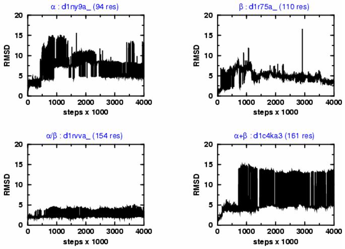
Showing the variation of the root mean square deviation of all C_α atoms (RMSD) from the native structure with the number of Monte Carlo iteration steps for four SCOP protein domains representing the four major structure classes: α (d1ny9a_), β (d1r75a_), α/β (d1rvva_), and α+β (d1c4ka3). Domains are described with the 3-point per residue model. All trajectories started from the crystal structures and were propagated for a total of 4,000,000 steps using an advanced combination of Parallel Tempering and Equi-Energy Monte Carlo methods. The simulation explore the conformational space around the native structure with rapid and frequent transitions between states that have very different RMSD values; at the end of the trajectories, the RMSD generally reaches values lower than 5 Å.

The 3pt per residue potential not only stabilized ∼80 % of all the studied folds, but introduced a rich diversity of native-like and partially denatured energy basins. As a consequence, folds represented by the 3pt model are metastable, and the sampled conformations are distributed among the dominant energy basin attractors around the native state. Note, that the above characteristics are not present in many commonly used simplified representations of protein structures (Supplementary Data, Figure 1). Specifically, for the all-α protein d1ny9a_, conformational regions up to ∼15 Å RMSD from crystal structure are explored first, then a rich diversity of conformational clusters are found in later stages of the sampling trajectory. Although the sampling path for a typical all-β protein, d1r75a_ starts with an initial ∼10 Å unfolding event, it is followed by a less eventful continuous deformation towards more native-like states. In this work, α/β proteins are found to be more stable, as typified by the progression of sampling events of d1rvva_ in Figure 1a. Finally, the figure shows the sampling events of an α+β protein d1c4ka3, which is very rich in diverse conformations involving structures 3 to 15 Å RMSD from native state.

Near-Native Energy Landscape

In general we find that domains of the same topological type possess a characteristic energy landscape fingerprint that depends on the given architectural fold class. Figure 1b illustrates these landscapes in the form of energy vs. RMSD plots generated from the near-native sampling trajectories of Figure 1a. It is clear from the figure that the dominant peaks in the RMSD distribution well describe the notable energy basins. In addition, the layout of native-like (0-5 Å) and far native (5-15 Å) favorable energy basins may carry information on conformational plasticity and the location of folding intermediates. For the all-α d1ny9a_, the most dominant energy basin was found to be at ∼5 Å, which is followed by two slightly less populated basins at ∼7.5 and ∼8.5 Å and a far-native but still significant basin at ∼12 Å. Contrary to the ordered layout of the all-α type energy landscape, the typical all-β domain d1r75a_, is more diffuse but there are still two well-populated energy basins. The stability of α/β domains is illustrated by d1rvva_, which has a dominant conformational cluster close to the crystal structure at 2 Å, and a less marked peak in the RMSD distribution at ∼4 Å. The RMSD distribution for the α+β domain d1c4ka3 is more like that of the all-α domains with two well-separated and comparably populated peaks.

Figure 1b.

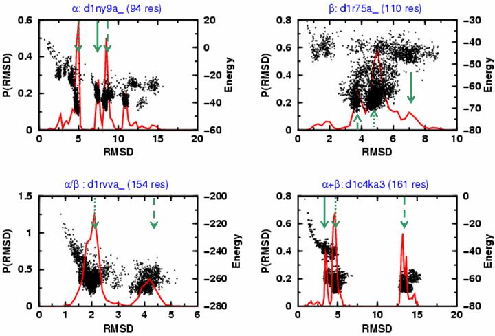
The distribution of RMSD values from native distribution (solid red curve) is plotted together with the energy values obtained for sampled conformations (black dots) for d1ny9a_, d1r75a_, d1rvva_ and d1c4ka3, the same protein folds shown in Fig. 1a. The green arrows indicate the locations of: (1) the most probable RMSD value (denoted RMS_A and marked with a dotted green arrow); (2) the second most probable RMSD value (denoted RMS_B, dashed green arrow); and (3) the third most probable RMSD value (denoted RMS_C, solid green arrow). In many cases, there is a clear separation of clusters of conformations based on their energy and RMSD values (d1r75a_, an all-β fold is an exception). The most probable cluster is often the closest to the native structure (i.e. RMS_A is smaller than RMS_B or RMS_C).

Representative set of domains

In order to quantitatively compare and describe the plasticity and stability of each of the 280 representative folds, the three dominant energy basins accessible to the search protocols are located based on the RMSD distributions. The procedures for locating the RMS maxima are described in the Methods section. Figure 1b shows the peak RMS values obtained from the RMSD distribution; it is clear from the figure that at most three dominant peaks capture many characteristics of the underlying distributions. We characterize each domain by the RMS values of dominant peaks, which correspond to the most populated conformational clusters.

In Figure 2a the RMSD of the most denatured but stable conformational energy basin (RMS_max = max(RMS_A,RMS_B,RMS_C)) is plotted as a function of the domain size showing that there is no correlation between the two quantities. For most of the cases (192 out of 280 or 68.57 %), RMS_max is below 6 Å and the average expectation value <RMS_max>, and standard deviation σ(RMS_max), are found to be 5.43 Å and 3.31 Å. In addition, there are significant variations among the fold classes, with <RMS_max>±σ(RMS_max) = 6.37±3.95 Å, 4.67±3.22 Å, 4.41±2.18 Å, 6.26±3.64 Å for all-α, all-β, α /β and α +β, respectively . These numbers clearly indicate, that all-α and the α+β domains have more low energy denatured states, whereas in all-β and especially α/β domains all the stable states are more native-like. In spite of their low mean value, the standard deviation for all-β proteins is close average. This is due to the fact to that all-β proteins tend to have either very low or very large RMS_max values (see Figure 2a). By contrast, the α/β proteins have a low mean RMS_max and standard deviation.

Figure 2.

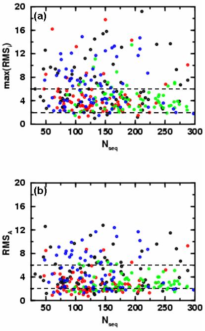
Showing the variation of the basin RMSD from crystal structure with the size of protein, (N_seq). We show the results for all 280 domains studied here: domains from α, β, α/β and α+β topological classes are colored black, red, green and blue, respectively. Here we consider the three most probable basins for each protein, RMS_A, RMS_B and RMS_C (see Fig. 1b). In (a) we show the RMSD value of the least native-like of the top three dominant energy basins (max(RMS_A,RMS_B,RMS_C)) as a function of the number of residues. One third of the domains (88 out of 280, 31.4 %) have RMSD values above 6 Å (dashed black horizontal line). On average α/β and β domains remain closer to the native state than other classes of domains. Only 4.29 % of proteins have RMSD values below 2 Å (dashed black horizontal line). 90 % of all-α, all-β, α/β and α+β class domains are below thresholds of 12.7 Å, 8.5 Å, 6.9 Å and 12.0 Å, respectively. In (b) we show the RMSD value of the most dominant energy basin (RMS_A) as a function of the number of residues. In this case, only 19.3 % (54 out of 280) of the domains have RMSD values above 6 Å (dashed black horizontal line) and almost all (66 out of 70 or 94.3 %) α/β domains are below the 6 Å line. 90 % of all-α, all-β, α/β and α+β class domains are below thresholds of 9.1 Å, 4.8 Å, 5.0 Å and 9.2 Å, respectively.

Figure 2b shows the location of the most dominant energy basin, RMS_A, as a function of the chain length. Most of the domains (226 out of 280 or 80.71 %) have RMS_A less than 6 Å. The average expectation value <RMS_A> and standard deviation σ(RMS_max) are found to be 3.92 Å and 2.39 Å. Again, there are significant variations among the fold classes, with <RMS_A>±σ(RMS_A) = 4.77±2.87 Å, 2.93±1.88 Å, 3.09±1.31 Å, & 4.89±3.08 Å for all-α, all-β, α /β and α +β, respectively. While the mean RMS_A value is smallest for the all-β class, the α/β class still has the smallest standard deviation. The RMS_A values of 90 % of all-α, all-β, α/β and α+β domains was found to be below 9.1 Å, 4.8 Å, 5.0 Å and 9.2 Å, respectively.

For 199 out of all 280 domains (71.1 %), RMS_A is less than RMS_max meaning that the more denatured conformations are less populated. In 27 cases (9.64 %) RMS_A is less but RMS_max is more than 6 Å, in addition (RMS_max- RMS_A) is at least 3 Å, indicating that these domains are featured with both stable highly denatured conformations and dominantly populated native-like states.

Figure 3a shows RMS_max as a function of fractional α-helix content, p_α. It is clear that domains with p_α content between 0.4 and 0.6 possess extra stability, with most RMS_max values below 6.0 Å. This finding does not depend on the fold class type. Figure 3b shows the variation of RMS_max with the relative terminal coil content. We find that domains with high secondary structure content do not occur below the dashed line RMS_max = 37.5*p_TC Å, where p_TC is the fraction of residues in the terminal loop regions (there are 8 exceptions out of 280 or 2.86 %). Thus, stable non-native orientations of the floppy terminal loops set a lower bound to the most denatured RMSD value.

Figure 3.

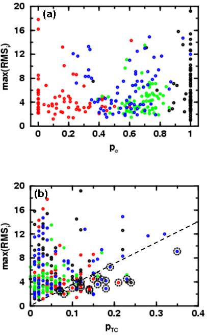
In (a) we show the variation of RSMD value of the least native-like of the top three dominant energy basins (max(RMS_i)) for all 280 protein folds as a function of the alpha content, defined as p_α = n_α/(n_α+n_β), where there are n_α residues in α-helix and n_β in β-sheet. In medium alpha content (0.4 < p_α < 0.6), most domains have cRMS values below 6.0 Å (there are only four exceptions). In (b) we show how the max(RMS_i)) varies with the fractional terminal coil residue content, p_TC (given by n_TC/n_seq, where n_TC is the number of residues before the first or after the last segment of α or β secondary structure). 259 out of the 280, (92.5 %) domains have few unstructured terminal residues (p_TC smaller than 0.15). In addition, as p_TC increases, so does the minimum RMSD of the most denatured basin from the native structure. Exceptions to this rule are found below the dashed guide line given by max(RMS_i)=15/0.4 p_TC and marked with a black dotted circle if they have lower than 50 % α and/or β content. Among the exceptions only 8 domains with high α and/or β content were found. Proteins from α, β, α/β and α+β topological classes are colored black, red, green and blue respectively.

Individual trajectories

In this section we carry out a detailed investigation of individual trajectories for domains with α (all-α), β (all-β), and mixed α+β content (α+β).

All-αclass

The representative sequence considered here is a 94 residue protein domain (d1ny9a_) with five helical segments joined together by loop regions. Figure 4 shows several aspects of the near native sampling, where Panels I-III contain the 2D projection of every 10000^th visited conformations generated by GRAPHVIZ.⁶⁹ In these panels, conformations are colored according to their relative energy values, RMSD from native state and history along the sampling trajectory, respectively. We note that the history of the sampling trajectory does not relate to any physical folding or unfolding event, neither does it carry any kinetic information at room temperature: it only orders the conformations based on their history of exploration. Right around the crystal structure, conformations have relatively high energy (Panel I), they are clustered in the 1 to 3 Å neighborhood of the native state and are visited only in the initial stage of the trajectory (Panel III). This set of conformations mostly belongs to cluster A, which is featured by representative conformation (A) depicted in Figure 4. According to Panel III, the later progress of the sampling path funnels into a set of scattered conformations with 13 to 15 Å RMSD from the native state (Panel II) and with still relatively high energy (Panel I). The snapshot of structure (B) from this region of the conformational space, shows that one helix is isolated and the rest of the helices form a highly compact globular state. In the next stages of sampling, cluster-like states of the conformational space, D and E are reached. These states are associated with a lower energy value. Further sampling explores conformational clusters, E, D and F, at ∼12.5, ∼8.6 and ∼5.0 Å away from the native state. Finally cluster G is located. It is very clear from the figure, that among these main conformational clusters, cluster F has the most native-like characteristics, the lowest energy and is the most populated cluster. The conformational characteristics of the alternative clusters D, E and G are well illustrated by the snapshots (Figure 4). The common pattern in each of these representative conformations is the presence of parallel/anti-parallel helix-helix interaction. In addition, structure D also contains stacking interaction between helices with perpendicular orientation and has a more compact character than structures E and G. As a result, D is the second most energetically favorable cluster (after cluster F). Interestingly, parallel and perpendicular helix-helix interactions are also present in the native state (N). Clearly structures with lower, more favorable energies are more native-like, validating the three-point energy function we use.

Figure 4.

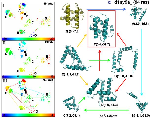
showing a two-dimensional projection of the high-dimensional conformational space of a typical all-α fold trajectory (d1ny9a_) in which the dots mark the positions of each structure as a function of x and y measured in Ångstroms. The projection was generated by using the open-source program GRAPHVIZ⁶⁹ with an all-to-all RMSD distance matrix derived from 400 structures sampled every 10,000^th steps along the trajectory. The native conformation is marked with N and various clusters of similar conformations are marked by letters from A to G. In panel (I), conformations are colored by their energy. We ensure uniform use of all colors by sorting the structures by the energy and linearly mapping the rank of each structure on the color scale (the minimum and maximum energy values are indicated). In panel (II), conformations are colored by their RMSD distance from the native structure; the clear progression from blue to red in each of the four directions (up, down, right, left) as points are further from the native conformation verifies the accuracy of our dimensional reduction. In panel (III), conformations are colored by the step number along the sampling trajectory. Since the most significant fraction of the trajectory and are located in some smaller clusters, a normalized square color-bar-timestep mapping is used in order to avoid the accumulation of multiple colors in narrow clusters. The latter non-linear monotonic scaling improves visualization of the progress along the trajectory. The single headed arrows between clusters point towards the lower energy cluster. In the right-hand panel, we show snapshots of typical conformations that represent the clusters shown in panels (I), (II) and (III). For each molecular structure we show in parenthesis the RMSD from native in Å and the total energy in kcal/mol. The conformation with the lowest energy (see (F)) is enclosed in a red box.

Since conformational clusters N and F are relatively close to each other, it is natural to ask if a simple conformational rearrangement can bring structure N to F (or vice versa). From the snapshots, such a rearrangement involves a relative rotation of two parallel surfaces, each defined by a pair of parallel helices. Such a conformational rearrangement is energetically unfavorable when the distance between the surfaces is fixed. This is in agreement with the near-native sampling, as there were no low energy conformations found close to the multidimensional “line” between clusters N and F.

All-β class

Contrary to highly structured energy landscapes that occur in the all-α class, typical β proteins show more diffuse energy landscapes. Figure 5 presents the example of a 108 residue protein domain, d1r75a_, showing the 2D mapping of the sampling trajectory initiated from the crystal structure. Panels I-III are created by the same sampling/analysis protocols used in Figure 4. Sampling of the conformational space starts with high energy states within 0 to 8 Å RMSD of the crystal structure (Panels I-III). The snapshot of one of the initial conformation is shown on the figure (A). Towards the middle of the path, conformations occupy a diffuse region between 3.8 and 6.0 Å RMSD from the native structure. The later region has lower energy than the rest of the conformational space (Panel I). The lowest energy conformation visited in the trajectory is shown in figure (B) and compared to the near-native state (N) in three different orientations. The comparison of energies and conformations for B, A and N again shows that low energy conformations tend to be native-like.

Figure 5.

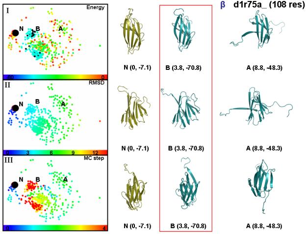
showing the same type of two-dimensional projection of conformational space used in Fig. 4 for a typical all-β fold trajectory (d1r75a_). In this case, conformational space has a more diffuse character. We demarcate by the letters N, A and B three regions of the conformational space representing the near-native states, the first quarter of the run and the final sixth of the trajectory. The left-hand panels, which are like those in Fig. 4, show how the conformation has a high energy at first and moves though much of the space before settling down close to the native structure in lowest energy basin B. The lowest energy conformation of the whole trajectory belongs to basin B and then a conformation for basin A is chosen as the lowest energy conformation among the top 2.5 % most denatured ones. The conformations associated with each basin and the native is shown in three different orientations to facilitate comparison to the native state. Each snapshots is shown with its RMSD values in Å and their total energy in kcal/mol.

α+β class

Figure 6 presents the sampling trajectory of two α+β folds, represented by a large domain d1c4ka3 with 161 residues and a smaller 55 residue domain (d1div_2), respectively. Panels I-III are constructed with the same methods used for Figures 4 and 5. Based on the occurrence of smeared, diffusive patterns in the 2D projected conformational distribution, α+β domains can be classified as being between all-α and all-β domains. The individual sampling trajectory of d1c4ka3 walks through high energy states 0 to 3 Å RMSD from the crystal structure, before settling down to three conformational clusters. The most denatured of these clusters (A) is about 15 Å from the native state and characterized with conformations having a compact “α+β” core region with the rest of the sequence partially unfolded. These types of denatured states could correspond to folding intermediates with “α+β” type nucleation sites. The two most energetically favorable clusters are A and B; B is the free energy minimum, with an average RMSD of 4.9 Å from native state.

Figure 6.

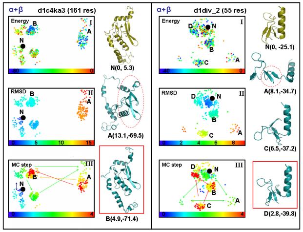
showing the same two-dimensional projection of conformational space used in Fig. 4 but now for two α + β domains, d1c4ka3, which has 161 residues, and d1div_2, which is much smaller with 55 residues. In the case of d1c4ka3, the two major conformational clusters are marked by A and B according to the order they were visited. The MC step subplot in panel (III) shows how the initially visited conformations (green nodes) transforms into orange and then finally red exploration paths (the single headed arrows between clusters point towards lower energy ones, the double headed arrows between clusters indicate their similar energy). The snapshots of the conformations show that the sampling path passes through a very unfolded state (basin A) before locating a near-native, low-energy conformation in basin B (framed in red). In the case of d1div_2, there are four major conformational clusters denoted A to D in the order visited. The representative conformations for each cluster are depicted. The snapshots of the conformations show that the simulation passes through very unfolded states (basins A and C) before locating an near-native, low-energy conformation in basin D (framed in red).

Figure 6 also depicts the sampling trajectory for a significantly smaller, 55 residue domain, d1div_2. Panel I shows that there are initial high energy conformations near the crystal structure. The sampling path then explores three conformational clusters with high energy; one of the most denatured clusters, A, contains conformations with a compact β-core. Finally, the three major conformational clusters, B, C and D are located. Here D is the most energetically favorable and most native-like cluster, with a conformation close to the native state. Again, many conformational clusters are located and the most native-like was found to have the lowest free energy.

Discussion

The use of multi-canonical sampling methods in the exploration of near-native energy landscape of proteins provides advantages to alternative approaches like high temperature unfolding.⁵⁴ In unfolding simulations, the temperature cannot be chosen arbitrarily high since the main objective is to infer folding paths at physiological temperatures. On the other hand, if the native state is kinetically trapped, very high temperature simulations are needed to produce unfolding events on a sufficiently rapid timescale. In multi-canonical methods,^49,51 there is no obvious restriction on the temperature of the most thermally activated system allowing the investigation of very stable native states. Another advantage of multi-canonical methods is that the replica of interest (300K) samples conformations according to the Boltzmann distribution at 300 K, whereas in unfolding simulations the visited conformations are sampled at a higher temperature. In spite of all the advantages one clear limitation of multi-canonical methods is their limited ability to provide direct kinetic information (knowledge of the free energy landscape does allow all kinetic pathways to be inferred). Multi-canonical methods are not only viable alternatives to explore the near-native energy landscape of proteins, but could be combined with unfolding simulations in a synergic way. For example, if a multi-canonical method locates conformational clusters A, B and C, unfolding simulations at different temperatures could be used to probe the energy landscape around each cluster and along a path between them.

The use of simplified protein models together with loop torsion angle flexibility is essential for efficient exploration of conformational space that is necessary if a large number of energy landscapes are to be investigated. In native proteins most of the conformational flexibility comes from loop segments, justifying our approximation of secondary structure elements as rigid bodies. This combination of rigid secondary structure with multi-canonical sampling has enabled our exploration of the near-native energy landscape for all the 280 representative fold domains with the 3 point per residue simplified representation.

The fictitious pathway generated by the current sampling protocols does not carry kinetic information, however as the conformational transitions sampled must occur in at least one of the different temperatures replicas, any two visited conformations must be connected kinetically at the highest temperature. This improved sampling comes at a price: the higher the temperature of the most thermally activated replica, the less the information that is preserved about kinetics at the temperature of interest. Nevertheless, for each representative domain the goals of the sampling protocol include (a) canonical exploration initiated from the native structure and (b) stochastic optimization to locate the most energetically favorable clusters of structures encircling the native state. We prefer canonical rather than the alternative stochastic optimization algorithms of simulated annealing, which only locates one conformation, and basin-hopping, which samples a transformed energy surface. Interestingly, when applied together with knowledge-based potentials, the present stochastic optimization approach is even further justified, since the underlying energy function has the character of a free-energy. In addition, tests on highly structured small proteins (<70 residues and <60 flexible loop torsion angles) (in preparation) show that a simulation starting from a completely unfolded state finds the same dominant energy basins. Investigation at this level is computationally prohibitive for our 280 domains, which were primarily chosen to represent protein fold space. Due to the limited kinetic information provided by our multi-canonical Monte-Carlo sampling, the order with which conformational clusters (low energy basins) are visited along the sampling path is not significant and could be different for different choices of random numbers.

The 3pt models used here is characterized with a rich variety of stable native-like or partially denatured energy basins. The basins could be biologically important in that (1) proteins need conformational flexibility for function; (2) stable partially denatured states could serve as intermediates between the native state and the unfolded ensemble.

Further analysis of the 3pt results was based on the location of the three most dominant energy basins. For those domains, where the RMSD of the most populated cluster (RMS_A) was more that 6 Å from the native state, we visually examined sampled conformations. We find six main causes, that include: (a) long terminal loop regions in the native structure; (b) long intermediate loop segments; (c) presence of non-native compact regions in the favored conformations, which often correlates with the formation of isolated substructures; (d) presence of relatively isolated compact super-secondary structures in the native structure; (e) biased relative orientation of small helices close to large, flat β sheets; (f) isolated secondary structure elements favored in native loop regions. It is important to note that while there was no correlation between the number of non-structured residues (not in α-helix or β-strand) and the RMS_A value, the distribution of non-structured residues along the sequence had more pronounced effect on stability (see Reason (2) above).

Another outstanding question is whether there are any plausible explanations for the different stability properties of different fold classes. We find that contacts in all-α domains are weaker and less specific than contacts in all-β domains (see Supplementary Figure 2). Thus, contrary to all-β domains, all-α domains can easily reorganize into partially denatured, stable and compact tertiary arrangements. In addition, the RMS_A for 90 % of all-α and all-β domains is below 9.1 Å and 4.8 Å, respectively. The detailed all-atom description of polypeptides also supports our observations in that since contacts between rigid β-strands have great strength and sharp orientation dependence due to hydrogen bond formation; in all-α proteins the H-bonds occur within the helix and weaker van der Waals interactions govern the inter-helix packing.

Unlike the α+β domains, α/β domains rarely contain contiguous α-helical secondary segments due to the alternation of α and β segments along the chain. Furthermore, large scale motion of α-helical segments in α/β domains is restricted by the strong interactions between consecutive β-strands that lock in the α-helix they surround. This is in agreement with our findings that α+β domains denature to a larger extent than α/β domains (<RMS_A>_α+β = 4.89 Å, <RMS_A>_α/β = 3.09 Å) and the RMS_A for 90% of α+β and α/β domains was found below 9.2 Å and 5.0 Å, respectively.

While all-β domains are found to denature to a slightly lesser extent than α/β domains (<RMS_A>_α/β = 3.09 Å, <RMS_A>_all-β = 2.93 Å), all-β domains have more variations in their stability (σ(RMS_A)_α/β = 1.31 Å, σ(RMS_A)_all-β = 1.88 Å). Consequently, all-β folds have slightly stronger stabilizing native contacts than α/β but a denaturing all-β fold is less likely to find a near native stable tertiary arrangement due to the strict orientation requirement of contacts between rigid β-strands. On the other hand, the broken β-strand-strand contacts in α/β domains can be locally stabilized by orientational independent helix-helix interactions.

Another interesting correlation was discovered between the RMSD of the most denatured energy basin and the α-helical content (p_α): for domains with p_α values between 0.4 and 0.6, most of the denatured clusters were not further than 6.0 Å away from native. This was generally true and did not depend on the fold class.

Conformational plasticity of the chains studied here was also revealed by focusing on the distribution of energy basins around the crystal structure. For some domains, the distributions were found to be diffuse, while others were surrounded by well isolated energy basins. The presence of diffuse landscapes correlated with the following three factors: (1) continuous deformation of loop elements, while preserving the relative arrangement of helices and sheets; (2) realignment of β-strands in a β-sheet; (3) rearrangement of compact and distantly isolated super-secondary structural elements. Domains contributing to factor (1) could belong to any topological class, but usually possess long loops (d1ig3a2, d1o50a1). Domains with factor (2) are mostly in the all-β (d1r75a_) or α+β (d1hdma2) classes; a good example for factor (3) is provided by d1el6a_, where continuous deformation of two compact super-secondary substructures occurs. In addition, factor (3) may occur due to the lack of long range interaction effects, which is the case for most of knowledge-based potentials.

The general layout of near-native conformations is clearly captured by the 2D scaling applied to representative conformations. Combining 2D maps with color representations of conformational properties like energy, RMSD and history of exploration provided a particularly good way to visualize near-native energy landscapes. Such conformational “maps” not only characterize how proteins approach the native state in a folding process, but also determine the properties of the native state and as such strongly relates to protein function. For example, proteins, which undergo large, function related conformational changes must possess more plasticity (even in loop torsion angle space, as the secondary structure of functioning proteins remains intact) at physiological conditions, and this property must be imprinted on the corresponding near-native energy landscape. While we characterize proteins with the 3pt representation, our analysis and visualization tools can be directly used for any conformational space in any representation.

Conclusions

In spite of the recent advances made in the development of novel sampling and optimization algorithms, the huge dimensionality of all-atom descriptions still limit the in silico investigations of large bio-molecular systems. There is clearly an increasing interest in approaches that foster the synergetic combination of new concepts and methods to overcome severe computational obstacles as the field rapidly progresses towards proteomics and system biology.

Our findings suggest there are realistic yet computationally tractable protein representations that when combined with state-of-the-art sampling protocols, enable studies to be conducted on families of proteins. Here the term ‘realistic’ embodies several properties, such as transferability across a large number of structures without knowing the native contacts, differences in the near-native properties of distinct folds, and sufficient conformational flexibility (a necessary requirement for protein function). In spite of the unique near-native energy landscape associated with each fold, several common patterns were discovered. Close similarity between the number residues being in α or β secondary structures (p_α ∼ 0.5), generally correlated with extra stability. Thus, the three point knowledge-based potential favored all proteins that were equally rich in both α and β secondary structural elements. In addition, a large number of unstructured terminal residues were generally found to be the main cause of large deviations from the native state.

The strength and specificity of native contacts among rigid secondary structure segments determines the stability and near-native energy landscape associated with the tertiary structure of each fold. Our findings imply that distinct stability properties of the different fold classes are due to from the strength and orientational specificity of interactions between β-strands as opposed to weak, non-specific interactions between α-helices.

Thorough investigation of some representative near-native energy landscapes from α-, β- and α+β-fold classes were performed by mapping a fraction of visited conformations onto a 2D space. Here, the simultaneous monitoring of various properties of conformational nodes, lead to a novel analysis towards the detailed visualization of conformational energy landscapes. The conformational distribution revealed that helically rich α-proteins have energy landscapes with many isolated energy basins, some of them belongs to globally rearranged alpha helical segments. On the contrary, highly structured β-proteins were found to have diffuse energy landscapes that only allowed for the local rearrangement of underlying β-strands.

Altogether, our findings imply, that the current knowledge based 3 point per residue representation captures some of the most important features of all-atom force fields (including specific hydrogen bonds). Thus, it provides a realistic picture of the forces shaping tertiary structure assembly in protein fold space. Consequently, the introduction of the present simplified energy/scoring function could potentially impact many diverse fields such as ab-initio structure prediction, threading, fold-recognition, study of large protein motion, protein-protein interactions among many others. In addition, the low energy and compact non-native conformations we found from fold space domains could open up new avenues in the large scale design of new folds or entire fold spaces. Finally, our tertiary sampling protocols combined with the current knowledge based potential are clearly powerful enough to become an integral element of a hierarchical structure prediction protocol.

Methods

Protein Structures

We randomly selected domains from 795 protein folds in SCOP-1.71 database,^2,57,58 covering the four major topological classes, all-α, all-β, α/β and α+β folds. The 70 single chain domains selected from each class have a range of lengths between 0 and 300 residues and an irregular secondary structure loop content of maximum 60 %. Altogether we studied 280 folds, more than one third of all known folds (∼35%). In addition, our 280 folds cover ∼45% of all folds and ∼75% of all α/β folds in our feature subset (up to 300 residues with maximum 60% coil residue content). The domain structures were obtained from the ASTRAL database,^53,59,60 http://astral.berkeley.edu/.

Models

The three-point knowledge-based model (3pt) follows on previous work (the list of 4500 known protein structures used is available as supplementary information).⁶¹ The three atoms used for each residue are the C_α carbon atom, the O carbonyl oxygen atom and a single side chain atom chosen to represent the center of mass of the side chain. The particular side chain atom used for a particular type of residue is taken as the atom that is most commonly closest to the actual center of mass of the side chain in known proteins. In this way we can use the knowledge-based energy functions derived for all-atom potentials and easily change the number of atoms used in the representation. The all-atom version of our force field has been extensively tested against commonly used physics based all-atom potentials.⁶ These three atoms have distinct types in different amino acids, so that the total number of atom types is 59, since Gly does not have a side-chain.

Since only torsion angle degrees of freedom are considered for the 3-point knowledge-based potential, intramolecular bonding or bending terms were not needed. To introduce additional flexibility into the model, no torsion angle potentials were used. We use two torsion angles per residue defined as C_α - O - C_α - O and O - C_α - O - C_α.

Selecting Conformations and Clustering

In order to obtain the structures presented on Figures 4-6, we used a very simple clustering approach.^62,63 Based on the representative conformations (400) from sampling trajectories, we evaluated the all-to-all RMSD distance matrix. Then, using an initial RMSD cutoff Δ, the structure with the largest number of neighbors marked the top cluster. In the next step the top cluster (structure and its neighbors) are eliminated and the procedure is continued until all structures are distributed among clusters. Here, Δ is chosen based on the RMSD distribution (e.g. for d1ny9a_, Δ = 1.5 Å is used). The conformations plotted on the Figures are the lowest energy conformations of individual clusters. In case of the diffuse conformational distribution of all-β domain d1r75a_, slight changes of Δ resulted on different top clusters. Therefore, on Figure 5 we only indicate the final lowest energy conformation and the lowest energy conformation found among the top 2.5 % most denatured structures.

Conformational Sampling

Multiple Temperature Markov Chains

The robust sampling methods employed here include parallel tempering⁴⁹ (PT) and the equi-energy sampler (EEMC).⁵¹ Both methods employ a sequence of Markov-Chains, X⁽⁰⁾, X⁽¹⁾,..., X^(K), ordered with increasing temperatures, T₀<T₁<...<T_K. As a result conformational exchanges between adjacent temperature Markov-Chains, conformations that are isolated by high energy barriers (permeable at T_K, but not at T₀) are visited at T₀. In parallel tempering, such exchanges take place between the instantly visited conformations of adjacent temperature chains. In equi-energy Monte Carlo, such exchanges take place between an instantly visited conformation and an ‘equal energy’ conformation obtained from the sampling history of the neighboring higher temperature chain. Here, two conformations R₁ and R₂ have ‘equal energy’, if E_i < E(R₁), E(R₂) < E_i+1, where an energy ladder {E_i, i=0,1,...,K} is chosen a priory⁵¹ and an initial approximation of the minimum attainable energy (E₀) of a given molecular system, enables the construction of the energy ladder for a given conformational sampling problem.⁵² Thus, EEMC allows exchanges between two conformations having similar energy, so that it can also connect low energy basins that are separated by large energy barriers. Note that by varying the type of the exchange (PT or EEMC), the two types of adjacent temperature replica swaps can be mixed on the fly.

It has been clearly shown⁵² that EEMC beats PT in locating multiple energy basins of noisy, low-dimensional, synthetic energy surfaces that include an off-lattice model protein.^64,65 Additional tests revealed that optimal performance across many different high dimensional problems is achieved with PT, but EEMC still has the beneficial property of potentially connecting distant energy basins. As the present study aims to explore different energy surfaces in a comparative manner, uniformly effective sampling is essential, we use a novel method that combines EEMC and PT and is called EEMC enhanced PT (see below).

Definition of Target Space, Sampling Protocols

To accelerate the canonical exploration of conformational space, we only vary the loop torsion angles between regular secondary structure elements (the definition of coil residues are obtained from native structures using STRIDE⁶⁶). For the 3 point per residue model, there are two torsion angle degrees of freedom for each residue, resulting in dimensionality, N_d, = 2*N_lr (N_lr is the total number of loop residues and N_d is less when there are loop residues at start or end of the chain). The individual Markov Chains (MC), X⁽ⁱ⁾ with temperatures, T_i, are propagated in N_d dimensional torsion angle space using a multivariate Gaussian: $X_{k+1}^{\left(i\right)}\sim N_d(X_k^{\left(i\right)},{\tau }_i^2{I}_n)$, and a proposed step size of the i-th order chain is taken to be ${\tau }_i=c\sqrt{T_i}∕I$, where l is the number of amino acids and c is optimized so that the acceptance ratio of the isolated MCs is about 0.4. Applying this proposal step size, we achieve a uniform acceptance ratio across different temperatures and proteins with various lengths.

For each domain, sampling is improved by using nine replicas with temperatures ranging from 300 to 900 K. We run trajectories by performing an initial 200,000 MC steps starting from the native state for each of the individual replicas without any multi-canonical exchange. This equilibration is followed by a multi-canonical production run of 4,000,000 MC steps to collect the statistics used in this study (this number of steps was found to be adequate to locate the most attractive near-native energy basins). For each Chain, the probability of a torsion angle change was set to p_MC = 1 - p_exch, where p_exch, the probability of adjacent temperature replica exchange was set to 0.05. The latter exchange was performed following either parallel tempering⁴⁹ or equi-energy Monte Carlo⁵¹ and the type of the exchange was sequentially changed along the trajectory; every 1000 steps of parallel tempering was followed by 200 steps of equi-energy Monte Carlo. For equi-energy Monte Carlo, E₀ (see. above) was approximated from a short preliminary sampling with parallel tempering. Although the focus of the present work is the effective exploration (stochastic optimization) of near-native low energy minima, the new protocol was rigorously tested to reproduce the analytical distribution of the synthetic one dimensional rough energy landscapes used in previous studies.⁵² Furthermore, some trajectories were regenerated using distinct pseudorandom sequences (different initial random number seed) and no significant differences were found between the visited conformational clusters.

Locating the maxima of RMSD distributions

In order to locate the three most dominant energy basins found for each protein, we use the distribution of RMSD obtained from near-native sampling. The three numbers are found by executing the following steps: (1) Find all the RMS values, where the distribution has a maximum value; (2) Set RMS_A, as the RMSD of the global maximum, RMS_B as the next and RMS_C as the third highest maxima. (3) If two maxima are closer than 0.5 Å, merge them and add one more maxima to the list.

Software

All cartoons of protein structures were generated by PyMol (http://www.pymol.org) using all-atom reconstructed protein models obtained using MAXSPROUT.⁶⁷ Multidimensional scaling was used by employing the algorithm of Kamada and Kawai,⁶⁸ which is implemented into the open source program GraphViz.⁶⁹ All sampling trajectories have been generated by the Palo Alto Sampler (Minary et al.). This software with all input parameters (including the tabulated knowledge-based potentials) needed to reproduce these results will be provided at http://csb.stanford.edu/~minary.

References

- 1.Ponting C, Russell R. The natural history of protein domains. Annu. Rev. Biophys. Biomol. Struct. 2002;31:45–71. doi: 10.1146/annurev.biophys.31.082901.134314. [DOI] [PubMed] [Google Scholar]
- 2.Murzin AG, Brenner SE, Hubbard T, Chothia C. SCOP:a structural classification of proteins database for the investigation of sequences and structures. J. Mol. Biol. 1995;247:536–540. doi: 10.1006/jmbi.1995.0159. [DOI] [PubMed] [Google Scholar]
- 3.Orengo CA, Michie AD, Jones S, Jones DT, Swindels MB, Thornton JM. CATH: a hierarchic classification of protein domain structures. Structure. 1997;5:1093–1108. doi: 10.1016/s0969-2126(97)00260-8. [DOI] [PubMed] [Google Scholar]
- 4.Holm L, Sander C. Mapping the Protein Universe. Science. 1996;273:595–602. doi: 10.1126/science.273.5275.595. [DOI] [PubMed] [Google Scholar]
- 5.Levitt M, Chothia C. Structural Patterns in Globular Proteins. Nature. 1976;261:552–558. doi: 10.1038/261552a0. [DOI] [PubMed] [Google Scholar]
- 6.Hou J, Jun SR, Zhang C, Kim SH. Global mapping of the protein structure space and application in structure based inference of protein function. Proc. Natl. Acad. Sci. USA. 2005;102:3651–3656. doi: 10.1073/pnas.0409772102. [DOI] [PMC free article] [PubMed] [Google Scholar]
- 7.Harrison A, Pearl F, Mott R, Thornton J, Orengo C. Quantifying the similarities within fold space. J. Mol. Biol. 2002;323:909–926. doi: 10.1016/s0022-2836(02)00992-0. [DOI] [PubMed] [Google Scholar]
- 8.Kihara D, Skolnick J. The PDB is a covering set of small protein structures. J. Mol. Biol. 2003;334:793–802. doi: 10.1016/j.jmb.2003.10.027. [DOI] [PubMed] [Google Scholar]
- 9.Zhang Y, Hubner IA, Arakaki AK, Shakhnovich E, Skolnick J. On the origin and highly likely completeness of single-domain protein structures. Proc. Natl. Acad. Sci. USA. 2006;103:2605–2610. doi: 10.1073/pnas.0509379103. [DOI] [PMC free article] [PubMed] [Google Scholar]
- 10.Sun ZB, Zou XW, Guan W, Jin ZZ. The architectonic fold similarity network in protein fold space. Eur. Phys. J. B. 2006;49:127–134. [Google Scholar]
- 11.Tiana G, Shakhnovich BE, Dokholyan N, Shakhnovich EI. Imprint of evolution on protein structures. Proc. Natl. Acad. Sci. USA. 2004;101:2846–2851. doi: 10.1073/pnas.0306638101. [DOI] [PMC free article] [PubMed] [Google Scholar]
- 12.Blackburne BP, Hirst JD. Three-dimensional functional model proteins: Structure, function and evolution. J. Chem. Phys. 2003;119:3453–3460. [Google Scholar]
- 13.Levitt M. Computer simulation of protein folding. Nature. 1975;253:694–698. doi: 10.1038/253694a0. [DOI] [PubMed] [Google Scholar]
- 14.Kolinski A, Skolnick J. Assembly of Protein Structure From Sparse Experimental Data: An Efficient Monte Carlo Model. Proteins. 1998;32:475–494. [PubMed] [Google Scholar]
- 15.Fain B, Levitt M. A Novel Method for Sampling Alpha-helical Protein Backbones. J. Mol. Biol. 2001;305:191–201. doi: 10.1006/jmbi.2000.4290. [DOI] [PubMed] [Google Scholar]
- 16.Zhang Y, Skolnick J. Automated structure prediction of weakly homologous proteins on a genomic scale. Proc. Nat. Acad. Sci. USA. 2003;101:7594–7599. doi: 10.1073/pnas.0305695101. [DOI] [PMC free article] [PubMed] [Google Scholar]
- 17.Jones DT, Liam JM. Assembling Novel Protein Folds From Super-secondary Structural Fragments. Proteins. 2003;53:480–485. doi: 10.1002/prot.10542. [DOI] [PubMed] [Google Scholar]
- 18.Haspel N, Tsai CJ, Wolfson H, Nussinov R. Reducing the computational complexity of protein folding via fragment folding and assembly. Protein Science. 2003;12:1177–1187. doi: 10.1110/ps.0232903. [DOI] [PMC free article] [PubMed] [Google Scholar]
- 19.Chikenji G, Fujitsuka Y, Takada S. Shaping up the protein folding funnel by local interaction: Lesson from a structure prediction study. Proc. Nat. Acad. Sci. USA. 2005;103:3141–3146. doi: 10.1073/pnas.0508195103. [DOI] [PMC free article] [PubMed] [Google Scholar]
- 20.Fujitsuka Y, Chikenji G, Takada S. SimFold Energy Function for De Novo Protein Structure Prediction: Consensus with Rosetta. Proteins. 2006;62:381–398. doi: 10.1002/prot.20748. [DOI] [PubMed] [Google Scholar]
- 21.Bowie JU, Luthy R, Eisenberg D. A method to identify protein sequences that fold into a known three-dimensional structure. Science. 1991;253:164–170. doi: 10.1126/science.1853201. [DOI] [PubMed] [Google Scholar]
- 22.Torda AE. The Proteomics Handbook. Humana Press; Totowa N.J.: 2005. Protein Threading; pp. 921–938. [Google Scholar]
- 23.Jones DT, Taylor WR, Thornton JM. A new approach to protein fold recognition. Nature. 1992;358:86–89. doi: 10.1038/358086a0. [DOI] [PubMed] [Google Scholar]
- 24.Levitt M. A simplified representation of protein conformations for rapid simulation of protein folding. J. Mol. Biol. 1976;104:59–107. doi: 10.1016/0022-2836(76)90004-8. [DOI] [PubMed] [Google Scholar]
- 25.Kolinski A, Skolnick J. Reduced models of proteins and their applications. Polymer. 2004;45:511–524. [Google Scholar]
- 26.Tanaka S, Scheraga HA. Statistical mechanical treatement of protein conformation. 1. Conformational properties of amino-acids in proteins. Macromolecules. 1976;9:142–159. doi: 10.1021/ma60049a026. [DOI] [PubMed] [Google Scholar]
- 27.Miyazawa S, Jernigan RL. Estimation of effective interresidue contact energies from protein crystal structures: Quasi-chemical approximation. Macromolecules. 1985;18:534–552. [Google Scholar]
- 28.Sippl MJ. Boltzmann’s principle, knowledge-based mean fields and protein folding. An approach to the computational determination of protein structures. J. Comput. Aided. Mol. Des. 1993;7:473–501. doi: 10.1007/BF02337562. [DOI] [PubMed] [Google Scholar]
- 29.MacKerrel A, Jr., Bashford D, Bellott M, Dumbrack RL, Evanseck JD, Field MJ, Fischer S, Guo H, Ha S, Joseph-McCarthy D, Kcuhnir L, Kuczera K, Lau F, Mattos C, Michnick S, Ngo T, Nguyen DT, Prodhom B, III, W ER, Roux B, Schlenkrich M, Smith JC, Stote R, Straub J, Watanabe M, Wiorkiewicz-Kuczera J, Yin D, Karplus M. All-atom empirical potential for molecular modeling and dynamics studies of proteins. J. Phys. Chem. B. 1998;102:3586–3616. doi: 10.1021/jp973084f. [DOI] [PubMed] [Google Scholar]
- 30.Cornell W, Cieplak P, Bayly C, Gould I, Merz K, Feguson D, Spellmeyer D, Fox T, Caldwell J, Kollmann P. A second generation force field for the simulation of proteins, nucleic acids and organic molecules. J. Am. Chem. Soc. 1995;117:5179–5197. [Google Scholar]
- 31.Karplus M, Weaver DL. Protein-folding dynamics. Nature. 1976;260:404–406. doi: 10.1038/260404a0. [DOI] [PubMed] [Google Scholar]
- 32.Mehta P, Heringa J, Argos P. A simple and fast approach to prediction of protein secondary structure from multiple aligned sequences with accuracy above 70 % Protein Science. 1995;4:2517–2525. doi: 10.1002/pro.5560041208. [DOI] [PMC free article] [PubMed] [Google Scholar]
- 33.Metropolis N, Rosenbluth AW, Rosenbluth MN, Teller AH, Teller E. Estimation of state calculation by fast computing machnies. J. Chem. Phys. 1953;21:1087–1091. [Google Scholar]
- 34.Tuckerman M, Berne BJ, Martyna GJ. Reversible multiple time scale molecular dynamics. J. Chem. Phys. 1992;97:1990–2001. [Google Scholar]
- 35.Minary P, Tuckerman ME, Martyna GJ. Long time molecular dynamics for enhanced conformational sampling in biomolecular systems. Phys. Rev. Lett. 2004;93:150201–150204. doi: 10.1103/PhysRevLett.93.150201. [DOI] [PubMed] [Google Scholar]
- 36.Li Z, Scheraga HA. Monte carlo-minimization approach to the multiple-minima problem in protein folding. Proc. Nat. Acad. Sci. USA. 1987;84:6611–6615. doi: 10.1073/pnas.84.19.6611. [DOI] [PMC free article] [PubMed] [Google Scholar]
- 37.Wales DJ, Doye JPK. Global optimization by basin-hopping and the lowest energy structures of Lennard-Jones clusters up to 110 atoms. J. Phys. Chem. A. 1997;101:5111–5116. [Google Scholar]
- 38.Voter AF. Hyperdynamics: Accelerated molecular dynamics of infrequent evnets. Phys. Rev. Lett. 1997;78:3908–3911. [Google Scholar]
- 39.Rahman JA, Tully JC. Puddle-skimming: An efficient sampling of multidimensional configurational space. J. Chem. Phys. 2002;116:8750–8760. [Google Scholar]
- 40.Rahman JA, Tully JC. Puddle-jumping: A flexible sampling algorithms for rare event systems. Chem. Phys. 2002;285:277–287. [Google Scholar]
- 41.Minary P, Tuckerman ME, Martyna GJ. Dynamical Spatial Warping: A novel method for the conformational sampling of biophysical structure. SIAM Journal of Scientific Computing. 2007 in review. [Google Scholar]
- 42.Swedensen RH, Wang JS. Nonuniversal critical dynamics in Monte Carlo simultions. Phys. Rev. Lett. 1987;58:86–88. doi: 10.1103/PhysRevLett.58.86. [DOI] [PubMed] [Google Scholar]
- 43.Tanner MA, Wong WH. The calculation of posterior distributions by data augmentation. J. Amer. Static. Assoc. 1987;82:528–550. [Google Scholar]
- 44.Minary P, Martyna GJ, Tuckerman ME. Algorithms and novel applications based on the isokinetic ensemble. I. Biophysical and path integral molecular dynamics. J. Chem. Phys. 2003;118:2510–2526. [Google Scholar]
- 45.Kirkpatrick S, Gelatti CD, Vecchi MP. Optimization by simulated annealing. Science. 1983;220:671–680. doi: 10.1126/science.220.4598.671. [DOI] [PubMed] [Google Scholar]
- 46.Nayeem A, Vila J, Scheraga HA. A comparative study of the simulated-annealing and monte carlo with minimization approaches to the minimum energy structures of polypeptides: Met-enkephalin. J. Comp. Chem. 1991;12:594–605. [Google Scholar]
- 47.Wales DJ, Scheraga HA. Global optimization of clusters, crystals and biomolecules. Science. 1999;285:1368–1372. doi: 10.1126/science.285.5432.1368. [DOI] [PubMed] [Google Scholar]
- 48.Brooks CL, Onuchic JN, Wales DJ. Taking a walk on a landscape. Science. 2001;293:612–613. doi: 10.1126/science.1062559. [DOI] [PubMed] [Google Scholar]
- 49.Geyer CJ. Computing Science and Statistics; Proceedings of the 23rd Symposium on the Interface; 1991.pp. 156–163. [Google Scholar]
- 50.Barhen J, Protoposecu V, Resiter D. Trust: A deterministic algorithm for global optimization. Science. 1997;276:1094–1097. [Google Scholar]
- 51.Kou SC, Zhou Q, Wong WH. Equi-Energy Sampler with applications in statistical inference and statistical mechanics. Annals of Statistics. 2006;34:1581–1619. [Google Scholar]
- 52.Minary P, Levitt M. Discussion of the Equi-Energy Sampler. Annals of Statistics. 2006;34:1638–1641. [Google Scholar]
- 53.Brenner SE, Koehl P, Levitt M. The ASTRAL compendium for protein structure and sequence analysis. Nucleic Acids Research. 2000;28:254–256. doi: 10.1093/nar/28.1.254. [DOI] [PMC free article] [PubMed] [Google Scholar]
- 54.Dagett V, Levitt M. A molten globulate state from molecular dynamics simulations. Proc. Nat. Acad. Sci. USA. 1992;89:5142–5146. doi: 10.1073/pnas.89.11.5142. [DOI] [PMC free article] [PubMed] [Google Scholar]
- 55.Kruscal JB. Multidimensional scaling by optimizing goodness of fit to a nonmetric hypothesis. Psychometrica. 1964;29:1–27. [Google Scholar]
- 56.Kruscal JB. Nonmetric mutidimensional scaling: a numerical method. Psychometrika. 1964;29:115–129. [Google Scholar]
- 57.Lo Conte L, Brenner SE, Hubbard TJP, Chothia C, Murzin A. SCOP database in 2002: refinements accommodate structural genomics. Nucl. Acid Res. 2002;30(1):264–267. doi: 10.1093/nar/30.1.264. [DOI] [PMC free article] [PubMed] [Google Scholar]
- 58.Andreeva A, Howorth D, Brenner SE, Hubbard TJP, Chothia C, Murzin AG. SCOP database in 2004: refinements integrate structure and sequence family data. Nucl. Acid Res. 2004;32:D226–D229. doi: 10.1093/nar/gkh039. [DOI] [PMC free article] [PubMed] [Google Scholar]
- 59.Chandonia JM, Walker NS, Lo Conte L, Koehl P, Levitt M, Brenner SE. ASTRAL compendium enhancements. Nucl. Acid Res. 2002;30:260–263. doi: 10.1093/nar/30.1.260. [DOI] [PMC free article] [PubMed] [Google Scholar]
- 60.Chandonia JM, Hon G, Walker NS, Lo Conte L, Koehl P, Levitt M, Brenner SE. The ASTRAL compendium in 2004. Nucl. Acid Res. 2004;32:D189–D192. doi: 10.1093/nar/gkh034. [DOI] [PMC free article] [PubMed] [Google Scholar]
- 61.Summa CM, Levitt M. Near-native structure refinement using in vacuo energy minimization. Proc. Nat. Acad. Sci. USA. 2007;104:3177–3182. doi: 10.1073/pnas.0611593104. [DOI] [PMC free article] [PubMed] [Google Scholar]
- 62.Torda AE, van Gunsteren WF. Algorithms for clustering molecular dynamics configurations. J. Comp. Chem. 1994;15:1331–1340. [Google Scholar]
- 63.Daura X, Gademann K, Jaun B, Seebach D, van Gunsteren WF, Mark AE. Peptide Folding: When Simulation Meets Experiment. Angew. Chem. Int. Ed. 1999;38:236–240. [Google Scholar]
- 64.Honeycutt JD, Thirumalai D. Metastability of folded states of globular proteins. Proc. Nat. Acad. Sci. USA. 1990;87:3526–3529. doi: 10.1073/pnas.87.9.3526. [DOI] [PMC free article] [PubMed] [Google Scholar]
- 65.Sorenson JM, Head-Gordon T. Redesigning the hydrophobic core of a model beta sheet protein: destabilizing traps through a threading approach. Proteins. 1999;37:582–591. doi: 10.1002/(sici)1097-0134(19991201)37:4<582::aid-prot9>3.0.co;2-m. [DOI] [PubMed] [Google Scholar]
- 66.Frishman D, Argos P. Knowledge-based protein secondary structure assignment. Proteins. 1995;23:566–579. doi: 10.1002/prot.340230412. [DOI] [PubMed] [Google Scholar]
- 67.Holm L, Sander C. Database algorithm for generating protein backbone and side chain co-ordinates from a Ca trace. J. Mol. Biol. 1991;218:183–194. doi: 10.1016/0022-2836(91)90883-8. [DOI] [PubMed] [Google Scholar]
- 68.Kamada T, Kawai S. An algorithm for drawing general undirected graphs. Information Processing Letters. 1989;31:7–15. [Google Scholar]
- 69.Ellson J, Gansner ER, Koutsofios E, North SC, Woodhull G. Graphviz and Dynagraph: Static and Dynamic Graph Drawing Tools. Springer-Verlag Graph Drawing Software. 2003:127–148. [Google Scholar]
Associated Data
This section collects any data citations, data availability statements, or supplementary materials included in this article.