Accurate prediction of protein–protein interactions from sequence alignments using a Bayesian method

Abstract

Accurate and large-scale prediction of protein–protein interactions directly from amino-acid sequences is one of the great challenges in computational biology. Here we present a new Bayesian network method that predicts interaction partners using only multiple alignments of amino-acid sequences of interacting protein domains, without tunable parameters, and without the need for any training examples. We first apply the method to bacterial two-component systems and comprehensively reconstruct two-component signaling networks across all sequenced bacteria. Comparisons of our predictions with known interactions show that our method infers interaction partners genome-wide with high accuracy. To demonstrate the general applicability of our method we show that it also accurately predicts interaction partners in a recent dataset of polyketide synthases. Analysis of the predicted genome-wide two-component signaling networks shows that cognates (interacting kinase/regulator pairs, which lie adjacent on the genome) and orphans (which lie isolated) form two relatively independent components of the signaling network in each genome. In addition, while most genes are predicted to have only a small number of interaction partners, we find that 10% of orphans form a separate class of ‘hub' nodes that distribute and integrate signals to and from up to tens of different interaction partners.

Introduction

A method that comprehensively and accurately predicts protein–protein interactions using only the amino-acid sequences of proteins would essentially allow the reconstruction of genome-wide interaction networks directly from genome sequences. Automated prediction of protein–protein interactions from their amino-acid sequences is therefore one of the great outstanding challenges in computational biology. Numerous approaches have already been proposed, which, apart from the amino-acid sequences themselves, use additional information as coexpression patterns, phylogenetic distributions of orthologous groups, co-evolution patterns, the order of genes in the genome, gene fusion and fission events, and synthetic lethality of gene knockouts (see Valencia and Pazos, 2002; Bork et al, 2004; Shoemaker and Panchenko, 2007 for reviews). There are, however, serious shortcomings to the currently existing methods. For instance, many of the approaches cannot infer direct physical interactions, but indicate only general functional ‘relationships', which may often be indirect and are difficult to validate. Some methods, such as those that rely on phylogenetic tree comparison, cannot be easily scaled up to large data sets. In addition, accuracy in genome-wide predictions is a general problem. Because true interactions are only a small fraction of the large number of possible interactions genome-wide, even relatively low false-positive rates lead to high numbers of false positives compared to the number of true predictions (see for example, Jansen et al, 2003). Furthermore, since high-throughput experimental methods for mapping protein–protein interactions are notoriously noisy, it is difficult to assess the reliability of computational predictions. This is especially a problem for transient protein–protein interactions such as those that take place during signaling. Yet these interactions are often most interesting because of their regulatory role.

Here we present a novel probabilistic method for inferring interaction partners in families of homologous proteins, using only alignments of amino-acid sequences. Of the existing methods for protein–protein interaction prediction, our method is most similar in spirit to the correlated mutations method of Pazos and Valencia (2002). In their approach, the assumption is made that, for interacting protein pairs, pairs of residues involved in the interaction will show correlated mutations. In particular, it is assumed that replacement of one of the interacting residues with a chemically highly dissimilar amino acid typically requires the other residue to also change substantially. For a given pair of proteins, orthologs from related genomes are collected and an ad hoc scoring scheme is used to identify pairs of positions that show significant correlation of their mutations across the orthologous pairs.

The similarity of this approach with ours is that we likewise assume that, for interacting protein pairs, there will be pairs of residues which show co-variation. However, whereas the method of Pazos and co-workers only considers one pair of proteins together with their orthologs at a time, we consider multiple alignments of entire families of proteins (or protein domains) that are known to interact, which includes all paralogs and orthologs at once. In addition, we use a rigorous Bayesian network framework to explicitly model the entire joint probability of all amino-acid sequences in the multiple alignments. In this model, the identity of each residue is probabilistically dependent on the identity of one other residue, which may either lie within the same protein or lie within the interacting partner. Our model also sums over all ways the residue dependencies can be chosen.

We demonstrate the power of our method by first applying it to bacterial two-component systems (TCSs) proteins, which are responsible for most signal transduction in bacteria. Whereas much knowledge has been gained in recent years regarding the structure of transcriptional regulatory networks and metabolic networks, very little is known about the global structure of signaling networks in bacteria. Here we provide the first genome-wide reconstruction of two-component signaling networks across all sequenced bacterial genomes. By comparing our predictions with large sets of known interactions, we demonstrate the high accuracy of our predictions. We further demonstrate the generality of the method by applying it to a recent data set of about 100 polyketide synthases (PKSs) (Thattai et al, 2007). This application also illustrates that our method can predict interaction partners with high accuracy even for relatively small datasets. Finally, our genome-wide predictions of two-component signaling networks across all sequenced bacteria allow us to make an initial investigation of the structural properties of these networks across bacteria.

Results

General model

Our method in general operates on sets of multiple alignments of homologous proteins (or protein domains) for which it is known that members of one multiple alignment can interact with members of another multiple alignment. To explain the model, we first describe it for the simplest possible case. In this situation, illustrated in Figure 1, there are two (large) families of proteins or protein domains, typically with multiple paralogous members per genome, for which it is known that in each genome each member of the first family interacts with one member of the second family. The set of all possible ‘solutions' for this problem corresponds to all possible ways in which we can assign, for each genome, each member of the first family to one member of the second family. In Figure 1, the alignments of the two families are shown side by side, with sequences grouped per genome from top to bottom. An assignment of interaction partners a corresponds to a vertical ordering of the sequences within each genome such that the sequences on the same horizontal ‘row' are assumed to interact. In this way, an assignment a implies a common multiple alignment of all sequences of both families.

Figure 1.

Illustration of the model used to assign a probability P(D∣a) to the joint multiple sequence alignment D of two protein families given an assignment a of interaction partners between them. Sequences from the same genome have the same color and horizontally aligned sequences are assumed to interact. The probabilities of pairs of alignment columns (ij) depend on the number of times n_αβ^ij that amino acids (αβ) occur in the corresponding columns. A dependence tree T and the corresponding factorization of the probability P(D∣a, T) of the entire alignment given the assignment and dependence tree is illustrated at the bottom of the figure.

We now calculate the probability P(D∣a) of observing the entire joint multiple alignment D of the sequences of both families in assignment a. We assume that, for each alignment position i, the probability to observe amino acid α at that position depends on the amino acid β that occurs at one other position j=π(i) (the ‘parent' of i). A dependence tree T (see Figure 1) specifies the parent position π(i) for each position i in the joint multiple alignment. The conditional probabilities p^ij(α∣β) are unknown parameters that are integrated out of the problem. As shown in Materials and methods, we can derive an explicit expression for the probability P(D_i∣D_j) of the entire alignment column i, given alignment column j in terms of the counts n_αβ^ij the number of times that the pair of amino acids (αβ) is observed at the alignment columns (ij). The probability P(D∣a, T) of the data, given dependence tree T, is then the product of conditional probabilities P(D_i∣D_π(i)) (see Figure 1) over all positions. The unknown dependence tree T is a so-called ‘nuisance parameter' and probability theory specifies (Jaynes, 2003) that to obtain P(D∣a), we should sum P(D∣a, T) over all possible dependence trees. Using an uniform prior over trees, this amounts to averaging P(D∣a, T) over all dependence trees (Meilá and Jaakkola, 2006). In cases where this summation is computationally intractable, we can also approximate P(D∣a) by finding the dependence tree T^* that maximizes P(D∣a, T^*) (see Materials and methods).

We sample the posterior distribution P(a∣D) over all possible assignments a using Markov chain Monte-Carlo sampling and keep track of the fraction f(m, m′) of sampled assignments in which proteins m and m′ are interaction partners. In the limit of long sampling, the frequencies f(m′, m) give the posterior probabilities P(m, m′∣D), that m and m′ interact. As explained in Materials and methods, this approach can be extended in several ways, including allowing more than two paralogous families and allowing for unequal numbers of members in the different families. These extensions are used for our predictions of two-component interactions below.

Application to TCSs

Bacterial TCSs are responsible for most of the signal transduction underlying complex bacterial behaviors (Grebe and Stock, 1999; Stock et al, 2000; Ausmees and Jacobs-Wagner, 2003). Although a lot is known about the TCS signaling for specific subsystems in a few model organisms, the interaction partners for the vast majority of TCS genes have not been determined experimentally. Comprehensive predictions of TCS-signaling interactions would thus provide important insights into how different bacteria respond to their environments, which regulons are under the control of which external signals, and which specific subsystems are connected by signaling pathways, with potentially important applications. For example, as TCS signaling is essential for host–pathogen interaction, insights into these interactions may have important applications related to human health. In addition, very little is currently known about the global structure of TCS-signaling networks across bacteria. With about 400 fully sequenced genomes available, comprehensive prediction of TCS-signaling networks across all bacteria would thus also provide a significant data set for studying the global structure of signaling networks in bacteria.

In its simplest form, a TCS consists of two proteins, a histidine kinase and a response regulator (Stock et al, 2000). The histidine kinase is in many cases a membrane-bound protein containing an extracellular sensor domain, which responds to environmental cues, and a cytoplasmic kinase domain. The kinase domain autophosphorylates upon the activation of the sensor, interacts very specifically with the response regulator, and transfers the phosphate to the regulator's receiver domain. Phosphorylation typically leads to the activation of the regulator, which often acts as a transcription factor.

For several reasons TCSs are particularly attractive for computational modeling. First, both histidine kinase and receiver domains exhibit significant sequence similarity and they can be easily detected in fully sequenced genomes using hidden Markov models (Bateman et al, 2004). Second, because TCSs are very abundant in the prokaryotic kingdom, with dozens of interacting pairs in some genomes and thousands of examples across all genomes, they provide enough data to detect subtle dependencies between the residues of interacting kinase/receiver domains. Finally, a significant fraction of all TCSs form so-called cognate pairs in which a single kinase/regulator pair lies within one operon in the genome. It is generally assumed that such cognate pairs are interacting kinase/regulator pairs, which is supported experimentally for a substantial number of pairs, and there are, to our knowledge, no examples that contradict this assumption. Therefore, the cognate pairs provide a very large data set of known interacting pairs that can be used to test the accuracy of the computational predictions. Additionally, they can be used as a ‘training set' for predicting interactions between all other kinases and regulators, that is, between ‘orphan' kinases and regulators which do not occur within an operon with their interaction partner.

We gathered an exhaustive collection of TCS proteins from 399 sequenced bacteria and multiply aligned all kinase and receiver domains. Whereas all receiver domains can be aligned in a single alignment, kinases show different domain architectures and we produced seven separate multiple alignments for the seven most abundant kinase domain architectures (see Materials and methods). We also divided the kinases and regulators into cognate pairs and orphans.

Determining interacting residues

The HisKA class is by far the largest class of kinases, with 3388 cognate HisKA/regulator pairs, corresponding to 72% of all cognate pairs, and we first investigated the evidence for dependencies between the amino-acid positions of the kinase and the receiver domains of this class. For each pair of positions (ij), where i lies in the kinase and j in the receiver, we quantified the ‘dependence' by the likelihood ratio R_ij between a model that assumes the amino acids at these positions are drawn from some joint probability distribution and a model that assumes they are drawn from independent distributions (see Materials and methods). This measure R_ij for dependence between positions i and j is closely related to the mutual information of the observed distribution of amino acids in positions i and j, which in turn is related to the statistical coupling between positions introduced in (Lockless and Ranganathan, 1999). As shown in the top left panel of Figure 2, almost 15% of all pairs of positions have a positive log(R_ij), which corresponds to over 1000 pairs. However, because our data set contains many examples of orthologous cognate pairs, we expect to see ‘spurious' correlations that are just the result of the evolutionary relationships between orthologous pairs. To investigate whether the high observed log(R_ij) values can be explained by phylogeny alone, we performed the following randomization. We collected sets of orthologous cognate pairs into orthologous groups and identified pairs of orthologous groups that occur in the same genomes. We then swapped kinase/regulator assignments between such pairs of orthologous groups. Thus, each kinase is now assigned to a wrong receiver domain, but the phylogenetic relations of all these ‘false pairs' are exactly the same as the phylogenetic relationships of the true cognate pairs. If all correlations were due to phylogeny, the distribution of observed R_ij values for the false pairs should be the same as that of the true pairs. As the top left panel of Figure 2 shows, the observed R_ij values for true pairs are much larger than can be explained by phylogeny. For example, only about 7% of false pairs show positive log(R_ij) and there are no false pairs with log(R_ij) larger than 235.

Figure 2.

Analysis of cognate pairs for the HisKA and H3 kinase classes. Top left panel: The red line shows the tail of the reverse cumulative distribution of log(R_ij) (dependency) values for pairs of positions in cognate HisKA kinase/receiver pairs. The blue line shows the tail of the log(R_ij) distribution after randomizing kinase/receiver assignments in such a way that all phylogenetic relationships are maintained. Top right panel: The cumulative distribution of estimated (see the text) distances between the amino acids in the co-crystal for the 50 pairs with highest R values (red line) versus all other pairs (green line). Bottom left panel: Sensitivities and positive predictive values of the predictions for cognate HisKA kinases and regulators. The red curves show the performance of the model in which P(D∣a, T) is averaged over all dependence trees, the blue curve shows the performance of the model P(D∣a, T^*) that uses only the best dependence tree, and the green line shows the performance of random predictions. All pairs of curves show estimated PPV±one standard error. Bottom right panel: Performance results as in the bottom left panel for cognate H3 kinases and regulators.

If the pairs of positions with large R_ij values reflect physicochemical constraints, we may expect that they are in close physical contact during the interaction of kinase and receiver. Although no structure of a HisKA kinase/regulator pair is currently available, the structure of the sporulation histidine phosphotransferase Spo0B with the response regulator Spo0F (Zapf et al, 2000) has been determined. Spo0B differs significantly in sequence from HisKA kinases, but can nonetheless be reasonably aligned to the HisKA Pfam profile. We used the Spo0B/Spo0F structure together with the Spo0B/HisKA alignment to estimate the physical distances between all pairs of positions in HisKA kinase/receiver pairs. The top right panel of Figure 2 shows that the pairs of positions with highest R_ij are significantly closer physically than other pairs (rank-sum test P-value 3 × 10⁻¹¹). In addition, Figure 3 shows the pairs of amino acids with the highest R_ij values on the Spo0B/Spo0F complex (black lines). It is striking that many of the positions that are predicted to depend on each other are indeed in close physical contact in the α-helices of the kinase and receiver domains (near the top right of the figure). Other interactions are predicted to occur between residues in an α-helix of the kinase domain and residues in loops of the receiver domain. A few of the predicted interactions are more puzzling: they involve residues not in close proximity, but the R_ij values are too high to be explained by phylogenetic dependencies. Some of these may be due to structural differences between the Spo0B/Spo0F complex and the HisKA/receiver complex, due to alignment errors, or indirect dependencies. In summary, the control for phylogenetic signal, the distances between pairs with high R_ij, and their location on a related structure all support that our R_ij scores capture meaningful functional dependencies between individual pairs of positions in kinase and receiver.

Figure 3.

Complex of the histidine phosphotransferase Spo0B (yellow) with the response regulator Spo0F (green) (Zapf et al, 2000). Only one half of the Spo0B dimer is shown. The site of autophosphorylation in Spo0B and the phosphorylation site in Spo0F are shown in blue. Out of the 20 HisKA/receiver pairs of residues with highest log(R_ij), 17 are shown as black lines (three cannot be displayed because the residues fall in gaps of the alignment with Spo0B). Amino acids marked in red are part of at least one of these 17 pairs.

Predicting cognate interactions

We next investigated how accurately the model can reconstruct known cognate pairs of HisKA kinases and their regulators. We collected the multiple alignments of all HisKA kinase domains and receiver domains from cognate pairs and sampled the space of all possible assignments, that is, all ways in which each kinase from each genome can be assigned to one regulator from the same genome. We sorted all predicted pairs by their posterior probability and measured, as a function of a cut-off in posterior probability, the fraction of all true cognate pairs that are among the predictions (sensitivity) and the fraction of all predictions that correspond to true cognate pairs (positive predictive value). These results are shown in the bottom left panel of Figure 2, both when approximating P(D∣a) using the tree with highest probability, that is, P(D∣a)=max_T P(D∣a, T) (blue curves), and when averaging over all dependence trees P(D∣a)=∑_T P(D∣a, T) (red curves). In the first approach, the dependence tree structure is calculated from the correctly paired cognate pairs before sampling, whereas in the second approach, no training set is used at all. In both approaches, the cognate pairs are reconstructed with high accuracy, but averaging over dependence trees performs clearly the best. This is not surprising since, as mentioned above, averaging over dependence trees is the correct way of treating the nuisance parameter T. Using only the best tree may amount to overfitting.

At 60% sensitivity, more than 95% (red curves) of the predictions correspond to true pairs. At a sensitivity of 75%, the fraction of predictions that are true pairs is still higher than 80% (red curves). This high accuracy is very striking, particularly considering that the algorithm is not given a single example of a true interacting pair, but infers all the cognate pairs in all genomes in parallel by searching for assignments that maximize the amount of dependency observed between the kinase and receiver sequences. We also predicted interaction partners for all cognate kinases and regulators of the H3 class, which is the second most abundant class (Figure 2, bottom right panel). In contrast to the HisKA class, for the H3 class there is a significant number of genomes with only a small number of H3 cognate pairs for which even random predictions would yield a reasonable fraction of correct predictions (green curves). However, it is still clear that our model reconstructs the cognate pairs with high accuracy, that is, at a sensitivity of 80%, more than 95% of the predictions (red curves) correspond to true pairs. In the Supplementary information, we show analogous curves for the other (smaller) classes of kinases which all show high accuracy of predictions, illustrating that the model can attain high accuracy on relatively small datasets. On the other hand, since for these smaller kinase classes there are often only a few cognate pairs per genome, the prediction problem is of course significantly easier. In summary, the results on cognate pairs suggest that, at least for cognate kinases and regulators, our algorithm can infer interaction partners ab initio with high accuracy.

Predicting orphan interactions

We are of course most interested in reconstructing those parts of bacterial two-component signaling networks that are currently not known, that is, to predict interaction partners for the thousands of orphan kinases and regulators. The prediction of orphan interactions is more difficult for two reasons. First, although for cognate pairs the assumption that each kinase and each regulator interacts mainly with one partner is probably not unreasonable, for orphan kinases and regulators this is less likely to hold. Many genomes contain unequal numbers of kinases and regulators, suggesting that at least some must interact with multiple partners. Second, a given bacterium typically contains orphan kinases from multiple classes, and we thus also have to infer which kinase class each of the orphan regulators belongs to.

To predict orphan interactions, we extended our model in several ways. First, we treat the multiple classes of kinases in parallel. Second, to account for unequal numbers of orphan kinases and orphan regulators, for a given assignment some kinases and/or regulators may remain without an interaction partner and these are scored separately (see Materials and methods). Finally, we add all the cognate pairs to the alignments of each class, with interaction partners correctly assigned, and keep these cognate pairs fixed. In this way the ‘frozen' cognate pairs act as a training set for the orphan assignments. The algorithm again uses Markov chain Monte-Carlo to sample over all ways of assigning orphan receivers to classes, and all ways of assigning orphan interaction partners in each class. Due to numerical difficulties in the extension of our model to multiple classes (see Materials and methods), we are unable to calculate the sum over all dependence trees with enough accuracy. Therefore, we use the cognate pairs to determine the best dependence tree and approximate P(D∣a) with max_T P(D∣a, T).

To benchmark the performance of this extended model we first used it to predict interacting partners for all cognate kinases and receivers, running on all seven classes in parallel. Since each cognate regulator is now allowed to switch dynamically between all seven classes of kinases, the search space of the extended model is much larger compared with the case in which each class is treated separately, and we expect this to negatively affect the performance. As shown in the Supplementary information, our predictions nonetheless remain quite accurate. Note also that for small classes, such as the HWE class, there is often only one kinase per genome and correct prediction amounts to identifying the regulator that belongs to the HWE class, which the extended model accomplishes with high accuracy.

Using our extended model, we then predicted orphan interaction partners genome-wide in all 399 bacteria. Currently very few orphan interactions have been measured experimentally. By far the most extensive knowledge is available for the interaction partners of HisKA orphan kinases in Caulobacter crescentus (Wu et al, 1999; Ohta and Newton, 2003; Skerker et al, 2005; Biondi et al, 2006). Table I compares our orphan interaction predictions in Caulobacter with those in the literature.

Table 1.

Comparison of our predictions for orphan HisKA kinases and orphan receivers with experimentally determined interactions in Caulobacter crescentus

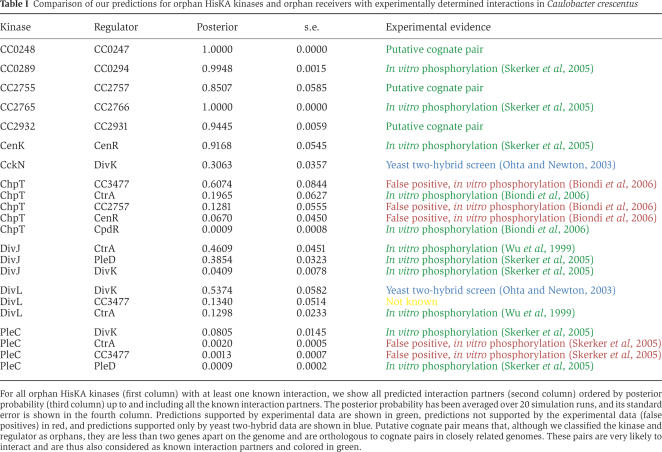Strikingly, for 10 of the 11 kinases with known interaction partners, the top computational prediction corresponds to a known interaction. In fact, of the 22 predictions in the table, which includes all 16 known interactions for these kinases, only five are at odds with current experimental data. Since there are 29 different orphan regulators in Caulobacter, that is, there are 29 interaction candidates for every kinase, this constitutes highly significant evidence that our method accurately predicts orphan interaction partners (P-value of 7.5 × 10⁻¹⁸; see Supplementary information). In the Supplementary information we also compare our orphan predictions with the few experimentally determined orphan interactions in Helicobacter pylori, Bacillus subtilis, and Ehrlichia chaffeensis.

Prediction of interactions between PKSs

PKSs are a family of bacterial proteins with extraordinary biosynthetic capabilities. Depending on very specific protein–protein interactions, they form multi-protein chains in which the order of the PKS proteins determines the order of monomers of the synthesized polyketide product. PKSs are of particular interest as, through genetic engineering of new PKS chains, they can potentially be used to achieve combinatorial biochemistry in the laboratory (Weissman and Leadlay, 2005).

The specificity of PKS interaction is believed to be determined by a small number of residues in the head (N-terminal) and tail (C-terminal). Here we focus on a data set of 149 interacting head–tail pairs published very recently (Thattai et al, 2007). Analysis of this data set has shown (Thattai et al, 2007) that both head and tail sequences can be phylogenetically clustered into three groups (H1 through H3 and T1 though T3), and that interacting pairs only occur between proteins from corresponding groups. Group membership can thus be used to predict which head and tail pairs are likely to interact.

We apply our method without any modification (i.e., as described in the General model section) to the above-mentioned data set. That is, we consider heads and tails as the protein families 1 and 2 (see Figure 1) and sample over all possible ways of assigning every head to exactly one tail within the same genome. This implies that heads of PKSs within one pathway are allowed to interact with tails of PKSs of a different pathway as long as they belong to the same genome, which is a harder and probably more biologically relevant problem than the one considered in (Thattai et al, 2007). The results are shown in the left panel of Figure 4. The red curve shows the performance of our model in which the probability of the data is averaged over all possible dependence trees, the blue curve shows the performance of a classification model that only takes into account the phylogenetic group information of the sequences (see Supplementary information), and the green curve shows the performance of random predictions. Note that although our model does not take into account any prior information about the phylogenetic grouping of heads and tails, it clearly outperforms the classification model used in (Thattai et al, 2007).

Figure 4.

Performance of predicted head–tail interactions for PKSs. Left panel: Sensitivities and positive predictive values of the predictions for all PKSs in the data set of Thattai et al (2007). The performance of our model in which P(D∣a, T) is averaged over all dependence trees is shown in red. The blue curve shows the performance if only the class information of heads and tails is used (see Materials and methods) and the green line shows the performance of random predictions. All pairs of curves show estimated PPV±one standard error. Right panel: Same as the left panel, but predictions restricted to the H1–T1 subclass.

Thattai et al (2007) have shown that within the largest group of interacting head–tail pairs (the H1–T1 group containing 90 pairs), there are a number of amino-acid residue pairs that lie close in the NMR structure of an interacting head–tail pair and that show significant evidence of co-evolution. However, attempts by Thattai et al (2007) to use these pairs of positions to predict interactions within the H1–T1 subclass yielded results that were only slightly better than random. In contrast, as shown in the right panel of Figure 4, our model shows excellent prediction accuracy on the H1–T1 subclass. This demonstrates that at least for some protein families our model obtains accurate predictions on data sets with less than 100 sequences.

The structure of two-component signaling networks across bacteria

Our genome-wide predictions of TCS-signaling interactions allow us, for the first time, to investigate and compare the structure of TCS-signaling networks across bacteria. However, in our cognate predictions above, we assumed each cognate to interact with only one other cognate, and the orphan predictions also assumed that orphans interact only with each other. As explained in the Materials and methods, to ensure that the network predictions are as comprehensive and unbiased as possible, we used a static scoring scheme that treats cognates and orphans equally (allowing for interactions between orphans and cognates) and allows an arbitrary number of interaction partners per protein.

Before investigating the predicted interactions we first investigated how the number of TCS genes of different types varies across genomes. As was shown by van Nimwegen (2003), the total number of TCS genes varies significantly between bacteria and scales approximately as the square of the number of genes in the genome, that is, whenever the total number of genes doubles, the total number of TCS genes roughly quadruples. Figure 5 shows the total number of cognates and orphans across genomes (left panel) and the number of orphan kinases and orphan receivers (right panel). There is a remarkably large variation in the relative number of orphans and cognates, that is, there are examples of genomes with tens of cognate pairs without any orphans, and vice versa genomes that have tens of orphans and no cognates. In addition, there appears to be little correlation between the number of cognates and the number of orphans. We also find no discernible correlation between the number of orphan kinases and the number of cognate regulators, or the number of orphan regulators and cognate kinases (data not shown). In contrast, as noted before (Alm et al, 2006), there is a clear correlation between the number of orphan kinases and the number of orphan regulators in a genome (right panel of Figure 5). These statistics provide a first suggestion that orphan kinases and orphan regulators might predominantly interact with each other rather than with cognates.

Figure 5.

Total numbers of cognates, orphan kinases, and orphan regulators across 399 sequenced bacterial genomes. Left panel: The total number of cognates (horizontal axis) versus the total number of orphans (vertical axis). Right panel: The number of orphan kinases (horizontal axis) versus the number of orphan regulators (vertical axis). Each dot in each panel corresponds to a genome. All axes are shown on logarithmic scale. To be able to show genomes with zero genes in one or more of the categories, 1 was added to each count, that is, one on the axis corresponds to a count of zero.

To investigate this further, we analyzed how the total number of predicted interactions depends on the number of TCS genes of different kinds. We distinguish four types of interactions: cognate–cognate interactions between cognate kinases and cognate receivers, orphan–orphan interactions between orphan kinases and orphan receivers, cognate–orphan interactions between cognate kinases and orphan receivers, and orphan–cognate interactions between orphan kinases and cognate receivers. For a genome with C cognate pairs, K orphan kinases, and R orphan receivers, there are, respectively T=C² cognate–cognate, T=KR orphan–orphan, T=CR cognate–orphan, and T=KC orphan–cognate interactions possible. For each genome, we determined the fractions f_cc, f_oo, f_co, and f_oc of all possible interactions in each class that are predicted to occur. For each category, we sorted the genomes by the total number of interactions T of that category, and by calculating running averages of the fractions (see Materials and methods) we determined the dependence of the fractions f_cc, f_oo, f_co, and f_oc on the total number of possible interactions T (Figure 6). If each possible interaction had a constant probability of being predicted, then the observed fraction of interactions would be independent of the total number of possible interactions T. In contrast, it is show in Figure 6 that all fractions decrease as a function of the total number of possible interactions T. To a reasonable approximation, all four fractions fall as a power-law of the total number of possible interactions T, with exponents −0.4 for cognate–cognate and orphan–orphan interactions, and −0.55 for cognate–orphan and orphan–cognate interactions.

Figure 6.

The fractions of interactions between cognates (red), between orphan kinases and orphan regulators (light blue), between cognate kinases and orphan regulators (green), and between orphan kinases and cognate regulators (purple) that are predicted to exist (vertical axis), as a function of the total number of possible interactions (horizontal axis). Both axes are shown on logarithmic scales. The values on the vertical axis were obtained by ordering genomes by the total number of interactions of each type, and taking running averages over 25 consecutive genomes. The widths of the curves correspond to two standard errors. The straight lines are power-law fits to the raw data and are given by f_cc=0.63T^−0.4, f_oo=0.50T^−0.38, f_co=0.41T^−0.55, and f_oc=0.39T^−0.55.

To investigate the consequences of this scaling for TCS network structure as a function of genome-size, let us first focus on cognate–cognate interactions. For a genome with N cognate pairs, there are T=N² possible interactions, of which a fraction T^−0.4 exists. The total number of cognate–cognate edges thus scales as T^0.6=N^1.2. That is, as the number of cognate pairs increases, the total number of interactions between cognates grows just a bit faster than linear. This implies that, although the total amount of cross talk between cognates is small, the amount of cross talk grows with the number of cognate pairs. In particular, the average number of interaction partners per cognate gene grows as N^0.2. To give an idea of the order of magnitude, for a genome with four cognate pairs the power-law fit predicts a total of 3.5 interactions, that is, essentially one interaction per gene. For a genome with 40 cognate pairs, a total of 56 cognate–cognate interactions are predicted, which amounts to 16 cross talks on top of the 40 cognate interactions. For orphan–orphan interactions, the numbers are very similar.

The power-law fits show that the fractions of cognate–orphan and orphan–cognate interactions decrease even faster with T. Consider for simplicity genomes with N cognate pairs, N orphan kinases, and N receivers. The total number of cognate–orphan and orphan–cognate interactions grows as N^0.9 in such genomes. Since this is slower than linear, it in particular implies that the average number of cognate–orphan and orphan–cognate interactions per gene decreases as N^−0.1. Apart from decreasing more rapidly with N, it is also shown in Figure 6 that cognate–orphan and orphan–cognate interactions are much less frequent than cognate–cognate and orphan–orphan interactions.

In summary, all our observations support the idea that orphans and cognates form two relatively separate TCS-signaling networks, that is, cognate–orphan and orphan–cognate interactions are relatively rare, and whereas the number of orphan–orphan and cognate–cognate cross-talks per gene increases with increasing network size, the number of cognate–orphan and orphan–cognate interactions per gene decreases with network size. As we saw above (Figure 5), this idea is also supported by the correlation in the number of orphan kinases and orphan receivers, and the absence of correlations between the numbers of cognates and numbers of orphans.

To provide additional evidence that orphans and cognates form relatively separate TCS-signaling networks, we mapped orthology relations of cognates and orphans across the 399 sequenced genomes (see Materials and methods; Supplementary information). We find that, whenever both genes of a cognate pair have orthologs in another genome, the two orthologs are also a cognate pair in this genome 99.1% of the time. In 0.6% of the cases, the orthologs of the cognate pair are both orphans, and in the remaining 0.3% of the cases one ortholog is a cognate and the other an orphan. In cases where only the kinase of the cognate pair has an ortholog, the orthologous kinase is a cognate 79% of the time. Similarly, if only the receiver of the cognate pair has an ortholog, then this orthologous receiver is a cognate 78% of the time. Finally, orthologs of orphan kinases are orphans 86% of the time, and orthologs of orphan receivers are orphans 80% of the time. Thus, although both cognate and orphan TCS genes undoubtedly share a common phylogenetic ancestry, our results intriguingly suggest that on shorter evolutionary time scales orphans and cognates evolve relatively separately from each other, and support our finding that the orphans and cognates form two relatively separate interaction networks.

To shed some light on the difference between orphans and cognates, we determined the connectivity, that is, the number of predicted interaction partners, for each TCS protein, and calculated the distribution of connectivities separately for all orphans and all cognates. Figure 7 shows the reverse cumulative distribution of kinases (left panel) and regulators (right panel). The figure shows striking differences between the connectivity distributions of cognates (red) and orphans (blue). First, for both kinases and regulators, the reverse cumulative distribution initially falls rapidly and roughly exponentially. In this regime, which includes roughly 90% of all genes, the connectivity distributions of cognates and orphans are very similar, although there are slightly more cognates with at least one predicted interaction partner than orphans. However, for the remaining 10% of genes the connectivity distributions of cognates and orphans are very different. In particular, there is a much larger number of orphans with high connectivity. For all four curves, but especially clearly for the orphans, there are two regimes in the distribution: one corresponding to relatively low-connectivity genes, which includes about 90% of all genes, and a second regime of high-connectivity genes, which covers the remaining 10%. It thus appears that, to a rough approximation, there are two types of TCS genes. Most kinases and regulators interact with only a few (less than five) partners, but about 10% interact with a large number of partners. The kinases in this class thus distribute a signal to a large number of downstream regulators, and the regulators in this class integrate a large number of input signals. Most of these ‘hub' kinases and regulators are orphans.

Figure 7.

Reverse cumulative connectivity distributions of kinases (left panel) and receivers (right panel). The fraction of genes with at least a given number of interaction partners (connectivity) is shown as a function of the connectivity. Cognates are shown in red and orphans in blue. The vertical axis is shown on a logarithmic scale.

Discussion

We have presented a novel general Bayesian network model for predicting interactions between families of interacting protein domains directly from amino-acid sequences. Our method incorporates several important methodological advances. First, the model does not require any training sets, but predicts interactions ab initio by sampling the space of all possible interaction assignments. For each interaction assignment the probability of the data is derived from first principles, that is, without any tunable parameters, and sums over all possible ways in which a tree of dependencies can be assigned to pairs of residues both within and between the interacting proteins (Meilá and Jaakkola, 2006). The latter is an important feature of the model. One might think that dependencies between residues within one protein are immaterial for the interaction with the other protein, and that equal or even better performance could be obtained by simply summing the dependencies of only those pairs of residues that go between the two interacting proteins. This is however not the case as the following example illustrates. Imagine two residues r and r′ in the first protein that both show clear dependence on a single residue q in the other protein, but that show even larger dependence on each other. Obviously, in this case it would be wrong to assume that the observed dependencies of q with both r and r′ are evidence that both r and r′ interact directly with q. Rather, q presumably interacts only with one of the these residues (say r) and the apparent dependency with r′ is a result of the strong dependency of r and r′ with each other. In contrast, if r and r′ were to show no dependency, then the observed dependency of q with both r and r′ would provide evidence that both residues interact with q. That is, the ‘meaning' of the dependency between any pair of residues depends subtly on the dependency that these residues have with all other residues and summing over dependence trees is the probabilistically correct way of taking all dependencies into account. Other important features are that we assign interaction partners for all proteins from all genomes in parallel, thereby maximizing the algorithm's ability to detect subtle sequence dependencies, and the use of Markov chain Monte-Carlo sampling to automatically obtain a measure of the reliability of each prediction.

Here we have applied our method to two bacterial protein families, TCS-signaling proteins and PKSs, which provide quite different challenges. In the case of the TCSs, we have thousands of examples, allowing the detection of subtle statistical signals. However, since the kinases naturally divide into subfamilies and receivers do not, receivers need to be both classified and matched to their interaction partners at the same time. In the case of the PKSs, we are dealing with only on the order of 100 homologous proteins, which makes the detection of dependencies between amino-acid residues much more difficult and requires careful statistical modeling. The fact that our algorithm successfully predicts interaction partners for both data sets demonstrates the generality of the method.

Our predictions of two-component interactions provide the first reconstruction of genome-wide signaling networks across all currently sequenced bacteria and our results suggest that these predictions have high accuracy (Figure 2; Table I). All predictions for each genome are available at the SwissRegulon web site (http://www.swissregulon.unibas.ch/cgi-bin/TCS.pl). Our predictions allow us to perform a first analysis of the structure of TCS-signaling networks across bacteria. First, we find that the average connectivity per gene increases slowly but significantly with the number of nodes in the network. Intriguingly, we find that cognates and orphans form two relatively independent groups, with cognates interacting predominantly with cognates and orphans predominantly with orphans. The latter observation is supported by an analysis of orthology relations, which showed that, at least on shorter evolutionary time scales, cognates and orphans evolve relatively independently of each other. Another significant finding is that, whereas 90% of TCS genes have a relatively small number of interaction partners, 10% of the orphans form a distinct class of ‘hub' nodes in the signaling networks, which have large numbers of interaction partners.

The finding that cognate and orphan TCSs form two relatively independent groups is further supported by a recent study by Alm et al (2006). They showed that kinases that have been horizontally transferred are more likely to be found in an operon with a response regulator than kinases that have been created by lineage specific expansion. This may partly explain the preferential cognate–cognate interaction as cognate kinases tend to be transferred with their interaction partners. However, it does not explain why ‘new' orphan kinases that have been created by duplication, evolve interaction specificity towards orphan regulators and rarely interfere with cognate systems. One may argue that cognate pairs form simple linear stimulus–response pathways that form a functional unit and are expressed (and transferred between genomes) as such. In contrast, TCS signaling in complex behaviors involving multiple in- and outputs would typically necessitate independent expression of the different components, especially if the processes involve temporal regulation of the interactions. This is in agreement with experimental evidence in Caulobacter, where orphans with generally multiple interactions control cell-cycle progression (Skerker and Laub, 2004), and in B. subtilis, where they are involved in sporulation (Fabret et al, 1999). In addition, our predictions suggest that indeed orphans are more likely than cognates to have high connectivity. However, it is clear that much more investigation is necessary to understand the reasons behind these global differences in interaction propensity between orphans and cognates.

There are many other examples to which our method can now be applied, that is, whenever there are two or more protein families or protein domains that interact we can apply the method to multiple alignments of these protein families/domains. Some examples to which the method can be applied in an essentially unaltered way are ABC ‘half transporters' (Higgins, 1992) or certain subfamilies of cytokines and their receptors (Kaczmarski and Mufti, 1991). Our results for the family of PKSs suggest that accurate predictions can also be obtained for fairly small protein families with on the order of 100 homologous sequences. However, the minimal number of sequences needed for reliable predictions is very difficult to estimate as it depends on many different factors. One of them is the entropy of the amino-acid distribution at different positions in the alignments, which has a strong influence on the strength of the co-evolutionary signal. For example, if only charged amino acids appear at two particular residues and positively charged amino acids preferably pair with negatively charged amino acids and vice versa, then only a very small number of sequences is needed to detect a dependency (the size of the alphabet is effectively reduced). In general it is probably safe to say that for any successful application, at least a few dozen examples are needed, and that a thousand examples should always be sufficient. In any case, as new sequences are becoming available at an ever-increasing pace we expect many protein families to become amenable to our analysis in the coming years.

Finally, the concept of dependence tree models may have very general applications. For example, hidden Markov models of protein domains and protein families score multiple alignments by assuming each alignment column is drawn from a weight matrix column that represents the propensities for different amino acids to occur at that position (Bateman et al, 2004). Our Bayesian network model provides a generalization of such scoring models to take into account dependencies between all pairs of positions in the alignment. Our method can thus be very generally applied to multiple alignments of protein sequences, for example, to infer interactions between residues, to discover subfamilies, and generally to improve multiple alignments of protein domains and families.

Materials and methods

We extracted the sequences of an exhaustive collection of TCS proteins from 399 sequenced bacterial genomes in NCBI (ftp.ncbi.nlm.nih.gov/genomes/Bacteria) using histidine kinase and response regulator profiles from the Pfam database (Bateman et al, 2004). Whereas there is only one Pfam profile for the receiver domains of response regulators, there are seven different kinds of kinase domains and kinases show a variety of domain combinations. The large majority of kinases falls into one of the eight domain architectures shown in Table II. Multiple alignments of all eight kinase classes and the entire set of receiver domains were produced using the program hmmalign (http://hmmer.janelia.org/). For the long hybrid class, we aligned only the Hpt domain, as the interaction is believed to take place mainly between this domain and the cognate receiver domain (Stock et al, 2000). The ATP-binding domain (HATPase_c) was not aligned, as it does not seem to be important for the kinase–receiver interaction (Ohta and Newton, 2003).

Table 2.

Pfam domain combinations of the most abundant kinase architectures and the number of times they occur in all 399 genomes

Name	Architecture	No. of cognates	No. of orphans
HisKA	HisKA, HATPase_c	3388	2158
H3	HisKA_3, HATPase_c	636	183
His_kinase	His_kinase, HATPase_c	245	23
Long hybrid	HisKA, HATPase_c, RR, (RR), Hpt	132	286
Short hybrid	HisKA, HATPase_c, RR, (RR)	126	985
Chemotaxis	Hpt, HATPase_c	89	77
Hpt	Hpt	37	192
HWE	HWE or HisKA_2, HATPase_c	34	162

RR stands for the receiver domain profile Response_reg. Both the short and long hybrid architecture can contain one or two receiver domains.

We defined operons as maximal sets of contiguous genes on the same strand of the DNA, with all intergenic regions between consecutive genes less than 50 bp in length. Whenever an operon contained only one kinase and one regulator, this pair was considered a cognate pair. Kinases (regulators) that did not sit in an operon with any regulators (kinases) were considered orphan kinases (regulators). We made separate alignments for the eight sets of receiver domains from cognate regulators that interact with each of the eight kinase domain architectures. As shown in the Supplementary information, in accordance with previous results (Grebe and Stock, 1999; Koretke et al, 2000), we observe that receiver domains that interact with different types of kinases show distinct amino-acid compositions, which can be used to predict what kind of kinase each receiver will interact with. Those results also indicated that Hpt and long hybrid receivers are very similar, and for the remainder of the analysis we fused these two classes into a single class.

Bayesian network model

We discuss first the simplest model setting: There are two families of proteins (or protein domains) X and Y that interact and we have multiply aligned all members of families X and Y from all sequenced genomes. We assume each member x of family X has precisely one interaction partner y of family Y in the same genome. An assignment a of interacting pairs can be thought of as specifying a joint multiple alignment D of the two families in which interacting members are aligned horizontally (Figure 1).

We calculate the probability P(D∣a) of the entire joint alignment given the assignment a and our model assumptions. Let D_i denote the alignment column at position i in the joint alignment, that is, i runs from 1 to L=L_X+L_Y, with L_X and L_Y representing the lengths of the family X and Y alignments. We first calculate the probability P(D_i∣ω) of the data D_i in column i given a weight matrix (WM) column ω:

where ω_α is the probability of seeing amino acid α at this position and n_αⁱ is the number of times amino acid α occurs in column i. Since we do not know the WM, we integrate over all possible WMs. Using a Dirichlet prior

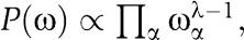we have

where n is the total number of amino acids in column i and λ is the pseudocount of the Dirichlet prior. Note that we treat gap symbols in the alignment simply as a twenty-first amino acid so that our alphabet size is 21.

Similarly, the probability P(D_ij∣ω) of a pair of columns given a weight matrix for the pair of columns is

where ω_αβ is the joint probability to see α at position i and β at position j, and n_αβ^ij is the number of times the pair of amino acids (αβ) occurs (on the same row) in columns (ij) of the alignment. Using again a Dirichlet prior

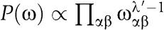and integrating out the unknown weight matrix ω, we have

The conditional probability of column i given column j is given by P(D_i∣D_j)=P(D_ij)/P(D_j). As shown in the Supplementary information, consistency requires that λ=21λ′, and we use the Jeffreys' or information geometry prior λ′=1/2 (i.e. uniform in the determinant of the Fisher information matrix). As a measure of dependence between two columns i and j, we use the ratio of likelihoods of the joint and independent models for the columns

For large counts n_αβ^ij the logarithm of R_ij is approximately proportional to the mutual information of the amino-acid distributions in columns i and j. For small counts, the ratio R_ij takes into account finite-size corrections. It also takes into account that the dependent model has more free parameters than the independent models. As a result, values of R_ij>1 can be interpreted as indicating positive evidence of dependence between positions i and j.

Let T denote a spanning tree in which each node is one of the positions i in the joint alignment. We (arbitrarily) pick one node r to be the root of the tree and direct all edges in the tree toward the root. In this directed ‘dependence tree' T each node i (except for the root) will have a single outgoing edge pointing to its ‘parent' π(i) (see Figure 1). Given an assignment a and dependence tree T, we calculate the probability P(D∣a, T) of the joint alignment by letting each column i depend on the parent column π(i). That is, we have

with r the root node and the product is over all nodes except for the root. Using (5) we can rewrite this as

where the first product is over all positions (including the root) and the second product is over all edges in the tree T. Note that only the second product depends on the assignment a and tree T, and that (7) is independent of the choice of the root and orientation of the edges in the tree. Note also that the position π(i) that position i depends on may lie either within the same protein or in the other protein.

To calculate the probability of the alignment independent of a particular dependence tree, we sum over all ∣T∣ possible spanning trees of the L positions:

As shown by Meilá and Jaakkola (2006), this sum can be calculated efficiently as a matrix determinant. Let M denote the Laplacian of the matrix R

from which one row and column have been removed. We then simply have

Given a uniform prior, P(a)=constant, over assignments, the posterior probability becomes proportional to the determinant, that is, P(a∣D)∝det(M).

Generalization: orphan predictions

The general model just presented can easily be generalized in various ways. Here we discuss the generalizations that we use to predict orphan interactions. Since genomes have typically different numbers of orphan kinases and orphan regulators, we have to relax the assumption that each protein has precisely one interaction partner. Although there are other possibilities, in our implementation we only consider assignments in which each protein is connected to at most one other protein at a time. For each genome we assign a number of interactions that is equal to the minimum of the number of orphan kinases and the number of orphan regulators. This typically leaves some proteins without an interaction partner. In addition, since there are seven kinase classes, with a separate multiple alignment for each, a full orphan assignment consists of seven joint alignments in parallel.

The probability P(D∣a) of the data given an orphan assignment is the product of the probabilities for each of the seven joint alignments of interacting pairs, the seven alignments of unassigned kinases, and seven alignments of the receiver domains of unassigned regulators. That is, we also divide unassigned receivers into seven classes. Let us focus on a single kinase class. We let J denote the joint alignment of the interacting pairs, with J^k the kinases in the joint alignment and J^r the receivers in the joint alignment. In addition, let K denote the alignment of unassigned kinases and R the alignment of unassigned receivers for this class. We now assume that we can factorize the joint probability of this data as follows

In particular, we will assume that the kinases in K were drawn from the same distribution as the kinases in J, and that the receivers in R were drawn from the same distribution as the receivers in J. We again write the conditional probabilities of unassigned kinases and receivers in terms of dependence trees T^k and T^r for the kinase and receiver positions. We then have

and

Note, however, that in both these expressions the numerator and denominator are entirely equivalent to expression (7). That is, these conditional probabilities can be calculated, using equations (2), (4), (5) and (7), in terms of the counts of the number of times different combinations of amino acids occurs in pairs of positions in the kinases K, the kinases J^k, the receivers R, and the receivers J^r.

We would in principle calculate the probabilities P(K∣J^k) and P(R∣J^r) by summing over all possible spanning trees T^k and T^r, which involves calculating determinants precisely as in equation (10). However, as described in the Supplementary information, numerical stability issues with the calculation of these determinants (see Cerquides and de Màntaras, 2003) force us to use an approximation when we run multiple kinases/receiver classes in parallel. Instead of calculating determinants, we thus approximate P(K∣J^k)≈P(K∣J^k, T^k) using the dependence tree T^k that maximizes the joint probability P(J^k∣T^k) of all cognate kinases in the class, and approximate P(R∣J^r)≈P(R∣J^r, T^r) by using the dependence tree T^r that maximizes the probability P(J^r∣T^r) of all cognate receivers in the class. Similarly, for the joint probability P(J) we also approximate P(J)≈P(J∣T^*), where T^* is the dependence tree that maximizes the probability of cognate kinase/receiver pairs in the class.

Finally, it is trivial to incorporate ‘training' examples of known interacting proteins in our Bayesian network model. We simply add the known interacting pairs to the alignments and keep these pairs fixed, that is, they are not sampled over. In our case, we added all cognate pairs for each of the seven classes to the corresponding joint alignments J. In this way the ‘frozen' cognate pairs in the alignment act as ‘seeds' that are used in sampling orphan assignments.

Gibbs sampling

To calculate the posterior probabilities P(x, y∣D) that members x and y interact, we sample the distribution P(a∣D) using a Markov chain Monte-Carlo method known as Gibbs sampling. We let r_g denote the maximum of the number of orphan kinases and the number of orphan regulators in genome g. We first sample a genome g with probability

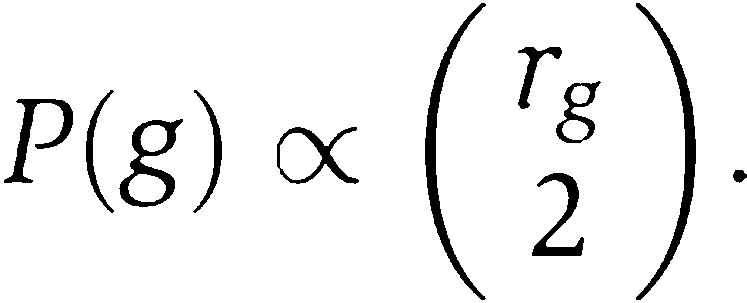If the sampled genome has more kinases than regulators, we pick two kinases (k₁, k₂) at random and sample over the current assignment and the assignment with the interaction partners of these kinases exchanged. Note that if one kinase is currently unassigned, the exchange would cause the other kinase to become unassigned. If both kinases are unassigned the move will leave the current assignment unchanged. If the sampled genome has more regulators than kinases we pick a pair of regulators (r₁, r₂) at random and again sample over the current interaction assignment and the assignment with the interaction partners swapped. If one or both of the regulators are unassigned, we also sample over the kinase class that each unassigned regulator is assigned to. That is, if both regulators are assigned we sample over two assignments, if one is unassigned we sample over 2*7=14 assignments, and if both are unassigned over 7*7=49 assignments. For the cognate predictions of Figure 2, the move-set simplifies since each protein is guaranteed to be assigned to precisely one interaction partner.

For each kinase/receiver pair (x, y) we then determine the fraction f(x, y) of sampled assignments that have x and y assigned as interaction partners. Note that, since we cannot assume that each orphan has only one interaction partner, these fractions cannot be directly interpreted as posterior probabilities of interaction. That is, if a certain kinase interacts 1/4 of the time with each of four different receivers this might simply indicate that this orphan kinase can interact with all four receivers. The results in Figure 2 were obtained by performing 5 independent sampling runs in each case, and averaging the observed frequencies f(x, y) from each of the runs.

Phylogenetic permutation test

To assess whether the high correlations seen between amino-acid pairs of kinases and receivers in the HisKA class could be explained by phylogeny alone, we constructed a null model that conserves all evolutionary relationships, but associates kinases with non-cognate regulators. We first map orthology relations between all cognate kinase/regulator pairs. Two cognate pairs are considered orthologs when they are best reciprocal hits and align over more than 80% of their lengths with at least 80% amino-acid identity. Next we filter out orthologous cliques, sets of orthologous cognate pairs that are all orthologous to each other. The result is a collection of n orthologs groups of cognate pairs. We define the overlap of a pair of orthologous groups as the number of genomes in which the representatives of both groups exist and produce a list of all pairs of orthologous groups sorted by overlap. Starting from the pair with highest overlap, we then create multiple alignments of ‘true' and ‘false' kinase/regulator pairs by applying the following rule for each entry in the list: We first check that both groups of cognate pairs have not yet been used. If not, we extract the sequences from the genomes in which both cognate pairs occur. These cognate pair sequences are added directly to the alignment of ‘true' pairs. The same kinase and receiver domain sequences are added also to the alignment of ‘false' pairs, but now with, in each genome of the group, the kinase of the first cognate pair assigned to the regulator of the second pair and vice versa. In this way the alignments of ‘true' and ‘false' pairs will consist of the same set of proteins with the precise same phylogenetic relationships between interacting pairs. We then determine R_ij for all pairs of positions from both ‘true' and ‘false' alignments.

Network structure analysis

Owing to the different overall number of TCS genes in the different kinase classes, both the sensitivity and specificity of the predictions will likely vary from class to class. As different genomes have different numbers of TCSs in different classes, combining predictions from all classes might introduce biases in our TCS network analysis. We therefore focus on the by far most common class of HisKA kinases and their receivers for the TCS network prediction and comparison. We first extracted all HisKA kinases from all genomes and all regulators that interact with HisKA kinases. For the latter, we took all regulators in cognate pairs with HisKA kinases as well as all orphan regulators that were classified as HisKA receivers during most of the Monte-Carlo sampling for the orphan predictions.

Whereas the Monte-Carlo sampling is most suited for predicting the most likely interaction partners of each kinase and regulator, it is not well suited for an unbiased inference of the entire signaling network in each genome, since the total number of interactions is fixed in each genome to at most one per protein per time point during the sampling. In addition, in the Monte-Carlo sampling only orphan interactions were sampled and cognate interactions were kept fixed. Therefore, to predict genome-wide TCS-signaling interactions allowing for an arbitrary number of connections, and treating cognates and orphans in the same way, we use the following procedure.

During the Monte-Carlo sampling runs that were used to predict orphan interaction partners, we also kept track of the numbers n_αβ^ij of interacting HisKA kinase/receiver pairs that have the combination of amino acids (αβ) at positions (ij). By averaging these over the sampling runs, we obtain the average counts 〈n_αβ^ij〉 that summarize the amino-acid composition at all pairs of position in predicted interacting HisKA pairs. Using the average counts 〈n_αβ^ij〉 we determined the position dependency statistics R_ij and determined three dependence trees T^*, T^k, and T^r that each maximize the sum of log (R_ij) along their edges. Whereas T^* takes into account all kinase and receiver positions, T^k only takes into account kinase positions, and T^r only the receiver positions, respectively. Finally we estimated the joint probabilities for amino-acid combination (αβ) to occur at positions (ij) as

The marginal probabilities p_αⁱ for amino acid α to occur at position i are given by summing the joint probabilities, for example,

Using these joint and marginal probabilities, we can then calculate, for any kinase-receiver pair with sequences S_k and S_r, respectively, the log ratio of the probabilities of their sequences (S_k, S_r) under the dependent model, that describes the probability distribution of all kinase and receiver positions in terms of the optimal tree T^*, and two independent models, that describe the dependencies of the kinase and receiver positions separately, using the optimal trees T^k and T^r, respectively. This ratio X(S_k, S_r) is given by the expression

with

where S_i is the amino acid that occurs at position i in the sequence S, and the sum is over all edges in the tree T. For each genome, we calculate the log ratio X(S) for all kinase-receiver pairs, including both orphans and cognates, and predict an interaction to occur between any pair for which X(S)⩾1. At the chosen (conservative) cut-off of 1, about half of all the predictions between cognate kinases and cognate receivers correspond to cognate pairs (see Supplementary information). To calculate the connectivity distribution, we counted the number of predicted interaction partners for each TCS gene and obtained reverse cumulative distributions separately for cognate kinases, cognate receivers, orphan kinases, and orphan receivers.

To determine the orthology relationships between cognates and orphans, we first extracted the sequences of all kinase domains belonging to HisKA kinases, as well as the sequences of all receiver domains of HisKA response regulators. For each kinase or receiver domain, we then identified orthologous domains in the 398 other genomes. A domain is considered an ortholog of domain when:

1. d and are each other's reciprocal best match.

2. d and align over 80% of their lengths.

3. d and are at least 60% identical at the amino-acid level.

Under these relatively stringent constraints, we typically find orthologous domains in between 4 and 10 other genomes. We then counted how often the orthologs of cognate pairs are themselves cognates pairs, how often only one of the members of a cognate pair has an ortholog, how often this single ortholog is itself part of a cognate pair, and how often it is an orphan, and so on. These ortholog statistics are shown in the Supplementary information.

For each genome, we determined the number of cognate pairs C, the number of orphan kinases K, and the number of orphan receivers R and determined:

1. The fraction f_cc of all T_cc=C² possible interactions between cognate kinases and cognate receivers that are predicted.

2. The fraction f_co of all T_co=CR possible interactions between cognate kinases and orphan receivers that are predicted.

3. The fraction f_oc of all T_oc=KC possible interactions between orphan kinases and cognate receivers that are predicted.

4. The fraction f_oo of all T_oo=KR possible interactions between orphan kinases and orphan receivers that are predicted.

For each category of interactions, we ordered all genomes with respect to the total number of possible interactions T. We then calculated running averages of both the f values and T values over windows of 25 consecutive genomes to determine the average dependence of f on T. s.e. of the running averages of f were also calculated by determining the variance var(f) of f across the 25 genomes in each window, and are given by

Finally, for each category we fitted f to a power-law function of T as follows. For a genome with T possible interactions, of which n are predicted to exist, we estimate f as f=(n+1)/(T+2) and logarithmically transform (T, f) to a data point (x, y)=(log(T), log(f)). We then fit a linear function y=ax+b to the set of data points (x, y) by finding the line that minimizes the average distance of the data points to the line (which is also the first principal component axis).

Supplementary Material

Supplementary Information

Supplementary Information

References

- Alm E, Huang K, Arkin A (2006) The evolution of two-component systems in bacteria reveals different strategies for niche adaptation. PLoS Comp Biol 2: e143. [DOI] [PMC free article] [PubMed] [Google Scholar]
- Ausmees N, Jacobs-Wagner C (2003) Spatial and temporal control of differentiation and cell cycle progression in Caulobacter crescentus. Annu Rev Microbiol 57: 225–247 [DOI] [PubMed] [Google Scholar]
- Bateman A, Coin L, Durbin R, Finn R, Hollich V, Griffiths-Jones S, Khanna A, Marshall M, Moxon S, Sonnhammer E, Studholme D, Yeats C, Eddy S (2004) The Pfam protein families database. Nucleic Acids Res 32: D138–D141 [DOI] [PMC free article] [PubMed] [Google Scholar]
- Biondi E, Reisinger S, Skerker J, Arif M, Perchuk B, Ryan K, Laub M (2006) Regulation of the bacterial cell cycle by an integrated genetic circuit. Nature 444: 899–904 [DOI] [PubMed] [Google Scholar]
- Bork P, Jensen L, von Mering C, Ramani A, Lee I, Marcotte E (2004) Protein interaction networks from yeast to human. Curr Opin Struct Biol 14: 292–299 [DOI] [PubMed] [Google Scholar]
- Cerquides J, de Màntaras RL (2003) Tractable Bayesian learning of tree augmented naive Bayes classifiers. Proceedings of Twentieth International Conference on Machine Learning. Menlo Park, California: AAAI Press [Google Scholar]
- Fabret C, Feher V, Hoch J (1999) Two-component signal transduction in Bacillus subtilis: how one organism sees its world. J Bacteriol 181: 1975–1983 [DOI] [PMC free article] [PubMed] [Google Scholar]
- Grebe T, Stock J (1999) The histidine protein kinase superfamily. Adv Microb Physiol 41: 139–227 [DOI] [PubMed] [Google Scholar]
- Higgins CF (1992) ABC transporters: from microorganisms to man. Annu Rev Cell Biol 8: 67–113 [DOI] [PubMed] [Google Scholar]
- Jansen R, Yu H, Greenbaum D, Kluger Y, Krogan NJ, Chung S, Emili A, Snyder M, Greenblatt JF, Gerstein M (2003) A Bayesian networks approach for predicting protein–protein interactions from genomic data. Science 302: 449–453 [DOI] [PubMed] [Google Scholar]
- Jaynes ET (2003) Probability Theory: the Logic of Science. Cambridge, UK: Cambridge University Press [Google Scholar]
- Kaczmarski R, Mufti GJ (1991) The cytokine receptor superfamily. Blood Rev 5: 193–203 [DOI] [PubMed] [Google Scholar]
- Koretke K, Lupas A, Warren P, Rosenberg M, Brown J (2000) Evolution of two-component signal transduction. Mol Biol Evol 17: 1956–1968 [DOI] [PubMed] [Google Scholar]
- Lockless SW, Ranganathan R (1999) Evolutionarily conserved pathways of energetic connectivity in protein families. Science 286: 295–299 [DOI] [PubMed] [Google Scholar]
- Meilá M, Jaakkola T (2006) Tractable Bayesian learning of tree belief networks. Statistics Computing 16: 77–92 [Google Scholar]
- Ohta N, Newton A (2003) The core dimerization domains of histidine kinases contain specificity for the cognate response regulator. J Bacteriol 185: 4424–4431 [DOI] [PMC free article] [PubMed] [Google Scholar]
- Pazos F, Valencia A (2002) In silico two-hybrid system for the selection of physically interacting protein pairs. Proteins 47: 219–227 [DOI] [PubMed] [Google Scholar]
- Shoemaker BA, Panchenko AR (2007) Deciphering protein–protein interactions. Part II. Computational methods to predict protein and domain interaction partners. PLoS Comput Biol 3: e43. [DOI] [PMC free article] [PubMed] [Google Scholar]
- Skerker J, Laub M (2004) Cell-cycle progression and the generation of asymmetry in Caulobacter crescentus. Nat Rev Microbiol 3: 325–337 [DOI] [PubMed] [Google Scholar]
- Skerker J, Prasol M, Perchuk B, Biondi E, Laub M (2005) Two-component signal transduction pathways regulating growth and cell cycle progression in a bacterium: a systems-level analysis. PLoS Biol 3: e334. [DOI] [PMC free article] [PubMed] [Google Scholar]
- Stock A, Robinson V, Goudreau P (2000) Two-component signal transduction. Annu Rev Biochem 69: 183–215 [DOI] [PubMed] [Google Scholar]
- Thattai M, Burak Y, Shraiman BI (2007) The origins of specificity in polyketide synthase protein interactions. PLoS Comp Biol 3: e186. [DOI] [PMC free article] [PubMed] [Google Scholar]
- Valencia A, Pazos F (2002) Computational methods for the prediction of protein interactions. Curr Opin Struct Biol 12: 368–373 [DOI] [PubMed] [Google Scholar]
- van Nimwegen E (2003) Scaling laws in the functional content of genomes. Trends Genet 19: 479–484 [DOI] [PubMed] [Google Scholar]
- Weissman K, Leadlay P (2005) Combinatorial biosynthesis of reduced polyketides. Nat Rev Microbiol 3: 925–936 [DOI] [PubMed] [Google Scholar]
- Wu J, Ohta JL, Newton A (1999) A novel bacterial tyrosine kinase essential for cell division and differentiation. Proc Natl Acad Sci USA 96: 13068–13073 [DOI] [PMC free article] [PubMed] [Google Scholar]
- Zapf J, Sen U, Madhusudan M, Hoch JA, Varughese KI (2000) A transient interaction between two phosphorelay proteins trapped in a crystal lattice reveals the mechanism of molecular recognition and phosphotransfer in signal transduction. Structure 8: 851–862 [DOI] [PubMed] [Google Scholar]
Associated Data
This section collects any data citations, data availability statements, or supplementary materials included in this article.
Supplementary Materials