Performance comparison between k-tuple distance and four model-based distances in phylogenetic tree reconstruction

Abstract

Phylogenetic tree reconstruction requires construction of a multiple sequence alignment (MSA) from sequences. Computationally, it is difficult to achieve an optimal MSA for many sequences. Moreover, even if an optimal MSA is obtained, it may not be the true MSA that reflects the evolutionary history of the underlying sequences. Therefore, errors can be introduced during MSA construction which in turn affects the subsequent phylogenetic tree construction. In order to circumvent this issue, we extend the application of the k-tuple distance to phylogenetic tree reconstruction. The k-tuple distance between two sequences is the sum of the differences in frequency, over all possible tuples of length k, between the sequences and can be estimated without MSAs. It has been traditionally used to build a fast ‘guide tree’ to assist the construction of MSAs. Using the 1470 simulated sets of sequences generated under different evolutionary scenarios, the neighbor-joining trees and BioNJ trees, we compared the performance of the k-tuple distance with four commonly used distance estimators including Jukes–Cantor, Kimura, F84 and Tamura–Nei. These four distance estimators fall into the category of model-based distance estimators, as each of them takes account of a specific substitution model in order to compute the distance between a pair of already aligned sequences. Results show that trees constructed from the k-tuple distance are more accurate than those from other distances most time; when the divergence between underlying sequences is high, the tree accuracy could be twice or higher using the k-tuple distance than other estimators. Furthermore, as the k-tuple distance voids the need for constructing an MSA, it can save tremendous amount of time for phylogenetic tree reconstructions when the data include a large number of sequences.

INTRODUCTION

A phylogenetic tree is a graphical representation of the genetic closeness among different species or biological entities. Despite other representation forms, such as phylogenetic networks (1), trees are still the most popular and standard representation of species’ evolutionary relationships. Many different criteria can be used to build a tree for a set of DNA sequences, such as maximum parsimony, minimum evolution, neighbor-joining (NJ), maximum likelihood and Bayesian inference. Among these methods, NJ is the most frequently used due to its high speed and comparable accuracy. Many modified versions of NJ algorithms (2) have been introduced since its introduction, such as bioNJ (3) and Weighbor (4).

The current paradigm in phylogenetic tree reconstruction is to start from a set of sequences, build multiple sequence alignment (MSA), and then based on the MSA, build a tree using one or several methods mentioned earlier. Therefore, clearly, all methods of phylogenetic tree reconstruction share the same starting point: computation of an MSA from the given set of DNA sequences. MSA refers to the arrangement of a set of sequences so that it reflects the evolutionary history of these sequences. Computationally, it is represented by a matrix, in which a row of the matrix represents one of the sequences in the set of sequences and a column represents specific positions along all the sequences and reflects matches, mismatches or gaps in all sequences. Therefore, once an MSA is constructed, an evolutionary hypothesis is automatically generated and represented by the alignment. The quality of an MSA thus directly affects the accuracy of subsequent phylogenetic inference, and erroneous MSA can lead to low-quality phylogenetic trees that give misleading information and false inference of evolutionary histories. Therefore MSA has been an extremely active research topic. More than 50 multiple sequence alignment methods and/or packages have been described over the past 10 years (5) and there were at least 20 new publications in 2005 alone (6). Among many MSA programs, ClustalW (7) is one of the most popular and standard programs. It made its way to daily usage by its friendly interface, stability and accuracy. However, as a result of its high consumption of time, it becomes impractical to use when the number of sequences that need to be aligned becomes large and/or the lengths of sequences reach a certain level. Subsequently, other programs have been introduced such as T-Coffee (8), MAFFT (9) and MUSCLE (10). Comparatively, the relatively new MUSCLE has the highest accuracy among existing programs and the shortest running time, according to the original paper (10).

However, despite the essential role of MSA in the entire process of phylogenetic tree reconstruction and multiple efforts to improve MSA methods, there remain several issues. First, finding the optimal MSA under a set of scoring schemes for a large number of sequences is computationally impossible. Most algorithms currently available are heuristic, which leads to an approximate solution. Even with heuristic methods, aligning a large number of sequences can be time consuming. Second, the quality of an MSA is extremely sensitive to the choices of the scoring parameters used in producing the alignment, such as penalty scores of gap opening and gap extension. Different scoring schemes can produce drastically different MSAs, which in turn can lead to different phylogenetic trees. Unfortunately, in most cases, the true MSA that reflects the evolutionary history of the underlying set of sequences is unknown. Thus the users have to either choose to trust the default scoring schemes or use their own judgment in choosing a scoring scheme. Third, the quality of an MSA is sensitive to sequence length difference and the degree of sequence identity. A set of sequences with dramatically different lengths can adversely influence the quality of an MSA. Similarly, if the sequences in the set are highly diverged from one another, the quality of an MSA is most likely low.

Because the construction of an MSA can introduce errors and adversely influence the accuracy of subsequent phylogenetic inference and because it is time consuming to construct an MSA for a large number of sequences, we formally introduce the application of the k-tuple distance (aka k-mer distance) in the phylogenetic tree reconstruction. The k-tuple distance refers to the total of the differences, over all possible k-tuples, between the sequences, for any given length k. The idea of using the k-tuple distance to construct a tree is not new and the procedure is in fact embedded in many MSA programs such as ClustalW (7), Kalign (11) and MUSCLE (10). To construct an MSA, these programs first compute a pairwise k-tuple distance matrix for the sequences to be aligned, use UPGMA or NJ methods to quickly build a ‘guide tree’, and use the guide tree to determine the order in which sequences or profiles are aligned. However, despite the common use of k-tuple distance in generating ‘guide trees’, guide trees are rarely used by evolutionary biologists as the final phylogenetic trees, and instead, packages dedicated to tree building such as PHYLIP (12) and PAUP (13) will be used to produce the final trees. To our knowledge, the value of the k-tuple distance in constructing a ‘real’ phylogenetic tree (instead of a ‘guide tree’ for sequence alignment) has not been formally discussed before, nor has the accuracy of the resulting phylogenetic tree. As the k-tuple distance can be calculated without sequence alignment and its computation for even a large number of sequences takes only seconds, k-tuple distance can be extremely useful when we are faced with the overwhelming number of sequences that require phylogenetic information and may essentially be the only option in cases where there are sequences that are too diverged to be reasonably aligned in the post-genomic era. But an important prerequisite for the broad application of k-tuple distance in phylogenetic tree reconstruction is that the trees built from the k-tuple distance have comparable accuracy to the trees built from traditional alignment-based methods.

In order to address the issue, we compared the k-tuple distance performance and accuracy in producing the correct NJ and BioNJ trees with four other commonly used distance estimators. The four distance estimators are model-based, in other words, they are computed based on certain substitution models for DNA sequence evolution. Our results show that when k equals five, the k-tuple distance outperformed other distance estimators most of the time and it could be twice, or more, the accuracy of other distance estimators. Moreover, compared to the existing alignment-dependent distance estimators, the k-tuple distance is fast and easy to compute and can save the tremendous amount of running time that is required for constructing MSAs. Taken together, our results show that the application of k-tuple distance in phylogenetic tree reconstruction is very promising.

MATERIALS AND METHODS

Simulation of five sequence datasets

We used DAWG (14) to simulate sequences. DAWG is a program that simulates the evolution of sequences based on a given phylogenetic tree, incorporating both nucleotide substitutions and insertions and deletions. It can simulate nucleotide substitutions with different substitution models and indel formation with a power law distribution of indel sizes. Therefore, it seems a rather good approximation of real sequence evolution. We simulated five different datasets of sequences using the HKY substitution model (15), as summarized in Table 1, in order to accommodate the different situations that we might encounter in real-world phylogenetic tree reconstruction. The first dataset is generated to consider the situation of alignment of regulatory regions or short intronic sequences and reconstruction of phylogenetic trees based on the alignment. Compared with coding sequences, regulatory regions and introns have much higher mutation rates and thus tend to be more diverse in both sequence composition and sequence length for a given set of genes. Therefore, aligning these sequences can be problematic, and the quality of the MSA is questionable and can be very low. In order to address this issue, we generated sequences with lengths ranging from 30 to 200 bp and insertion and deletion rates of 0.1, respectively. We generated random trees and used them as model trees to generate sequences. For these sets of sequences, we tested the performance of the k-tuple distance in dealing with short and divergent sequences. The second and third datasets consisted of sequences of different lengths (500–1500 bp), which accommodate the common situation of phylogenetic tree reconstruction. The only difference between these two sets was the source of model trees for simulations. Dataset 2 used real trees downloaded from the TreeFam database (16) as model trees while dataset 3 used randomly generated trees for sequence simulation. For dataset 2, we randomly selected 210 real trees from the TreeFam website. We chose 200 trees with the number of sequences within the interval of 50–250 and 10 trees with the number of sequences larger than 250. For example, trees 1–10 have 50–60 sequences, trees 11–20 have 61–70 sequences, trees 21–30 have 71–80 sequences and so on. For dataset 3, we generated random trees using the bioperl module RandomFactory. The difference between real trees and random trees lies in the branch lengths, which will in turn affect multiple sequence alignment. Datasets 4 and 5 consisted of simulated sequences with the same length, thus accommodating the situation of highly similar sequences in the real world. It is an ideal situation, but we used it as a boundary situation. Dataset 4 used real trees as model trees, and dataset 5 used random trees as model trees.

Table 1.

Summary of the 1470 simulated sets of sequences

Datasets	No. of Trees	Types	Indel rate	No. of Taxa	Length (bps)
1	210	Random	0.2	50–260	30–200
2	210	Real	0.1	50–250 and 10 trees with taxa >250	50–1500
3	210	Random	0.1	50–260	500–1500
4	210	Real	0	50–250 and 10 tree with taxa >250	500–1500
5	210	Random	0	50–260	500–1500
6	210	Real	1	50–250 and 10 trees with taxa >250	500–1500
7	210	Real	10	50–250 and 10 trees with taxa >250	500–1500

The length of a simulated sequence is a random number within the range specified below.

Computation of five distance matrices

The k-tuple distance is calculated as the difference in the frequencies of all possible tuples of length k. We calculate the k-tuple distance by moving a sliding window of length k over the sequence with 1 bp overlapping step size and counting the number of occurrences of tuples of length k. For example, when tuple size k is 3, we need to count the number of occurrences of 64 possible tuples in a DNA sequence. Therefore, each sequence can be represented by a vector containing 4^k (k is the tuple size, k ≥ 1) numbers, each of which represents the frequency of the corresponding tuple in the sequence. For any two sequences X and Y, the k-tuple distance is calculated using the formula: , where X_i and Y_i correspond to the tuple i's frequencies (=counts/n−k + 1) in sequences X and Y, respectively; n is the sequence length of either sequence X or Y; k is the tuple length. Therefore, the k-tuple distance takes into account the sequence length difference. We compared tuples of different sizes and found that tuple size 5 combines both performance speed and accuracy; tuples of shorter lengths contain less information and include more randomness; tuples of longer lengths contain more information and less randomness, but the vector size expands exponentially and gets too large and computationally inefficient. We observed combined optimum when the length is 5. There was a slight performance drop when the length was raised to 6 (data not shown here) [though we suggest no particular interpretation in terms of biological process or structure of 5-tuples versus other k-tuples, it would seem that 5-tuples constitute more precise genomic signatures than dinucleotides as studied, e.g. in (17,18)].

Because the k-tuple distance plays the same role as other distance estimators in phylogenetic tree reconstruction, the procedure of producing trees using the k-tuple distance is the same as for other distance estimators, that is, first build a pairwise k-tuple distance matrix for a set of sequences, and then construct a phylogenetic tree based on the distance matrix using a distance-base tree-building method. As we chose tuple length 5, we obtained a vector of 1024 numbers representing the frequencies of all 1024 possible tuples for a specific sequence. We constructed the k-tuple distance by adopting Euclidean distance to measure distances between two sequences. As the distances in the matrix are computed on percentages and thus small, we amplified it by 1000, which has no effect on subsequent analyses.

We compared the performance of the k-tuple distance with four other distance estimators including F84 (19), Jukes–Cantor (20), Kimura (21) and Tamura–Nei (22). We used MUSCLE to compute MSAs for all the simulated sets of sequences. We calculated the F84, Jukes–Cantor and Kimura distance matrices through the dnadist program in PHYLIP (12) and the Tamura–Nei distance matrix through PAUP (13).

Performance comparison of five distance estimators using symmetric distance

Since the focus of our study is to compare the performance of the k-tuple distance with existing distance estimators in phylogenetic tree reconstruction, we used only two very popular methods to perform tree reconstruction, the standard NJ program in PHYLIP (12) and BioNJ (3). BioNJ has been shown to be the best NJ method (23). In total, we have 10 different combinations of tree reconstruction algorithms and distance metrics.

We measured the accuracy of underlying distance estimators by comparing each NJ tree with the original model tree used by DAWG to generate sequences. Strictly speaking, the accuracy for the four distance estimators also includes the accuracy of the MSA. We used the symmetric difference (SD) (24) for this purpose. SD is bounded from zero to 2(t − 3), meaning identical to totally different respectively, where t is the number of taxa in the trees. It is a commonly used and standardized measurement of ‘topological closeness’ between different trees. Mathematically speaking, the symmetric difference of two sets was the number of the sets of elements that are in one but not the other set. For example, when comparing two trees built from 10 taxa, a score between 0 and 14 will be returned, with 0 meaning identical or isomorphic and 14 meaning completely different. The result was transformed into accuracy in percentage by the following formula.

1

Where S_i is the SD score of a particular entry and S_max is the largest score possible for that particular comparison. All trees are taken as unrooted trees in our study.

RESULTS

We simulated 1050 sets of sequences with the number of sequences ranging from 50 to 250 or more and with different settings for indel rates and sequence lengths (Table 1). We constructed both NJ and BioNJ trees for each set of sequences and found that they gave qualitatively the same results in terms of the comparison between the k-tuple distance and the other four distance estimators. For brevity, we show only the results of NJ. The results of BioNJ are summarized in Table 2.

Table 2.

The average accuracy (A) and standard deviation (S) of all possible combination between tree building methods and distance estimators

Name	Type	NJ							BioNJ
		Dataset 1	Dataset 2	Dataset 3	Dataset 4	Dataset 5	Dataset 6	Dataset 7	Dataset 1	Dataset 2	Dataset 3	Dataset 4	Dataset 5
k-tuple distance	A	0.26110	0.51568	0.30889	0.52836	0.33298	0.40770	0.16618	0.26090	0.51966	0.30846	0.53144	0.33285
	S	0.04463	0.09604	0.04278	0.10363	0.04744	0.09988	0.07410	0.04407	0.09773	0.04266	0.10316	0.04766
Tamura-Nei	A	0.11246	0.35853	0.16092	0.58316	0.25570	0.14186	0.04860	0.10977	0.38250	0.16134	0.60882	0.25466
	S	0.03687	0.19900	0.03402	0.20987	0.04321	0.08386	0.02595	0.03662	0.19207	0.03489	0.19781	0.04212
F84	A	0.00126	0.42550	0.04410	0.50200	0.07833	0.15035	0.02973	0.00144	0.43291	0.04274	0.51339	0.07830
	S	0.00471	0.18174	0.08308	0.17209	0.12747	0.14348	0.04503	0.00496	0.18516	0.08145	0.17759	0.12823
Jukes-Cantor	A	0.00043	0.43574	0.03222	0.64871	0.06525	0.14376	0.02238	0.00092	0.43934	0.03231	0.65129	0.06470
	S	0.00189	0.20702	0.07173	0.18384	0.12097	0.15540	0.04173	0.00380	0.21054	0.07228	0.18542	0.11992
Kimura	A	0.00103	0.42759	0.04484	0.50406	0.08002	0.15236	0.03014	0.00144	0.43457	0.04414	0.51556	0.07978
	S	0.00448	0.18031	0.08374	0.17061	0.12899	0.14257	0.04510	0.00486	0.18345	0.08259	0.17731	0.12914

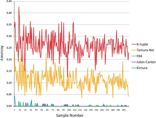
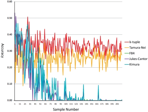
Alignments for short sequences such as upstream regulatory regions can be extremely difficult due to the lack of knowledge on their mutation patterns. Low alignment quality can lead to erroneous inference of phylogenetic trees for these regions. Because using the k-tuple distance matrix to build phylogenetic trees bypasses the construction of an MSA, the k-tuple distance has great potential in addressing the need of tree construction for these regions. To evaluate the k-tuple distance performance in short sequences, we simulated 210 sets of sequences with the number of taxa in the sets ranging from 50 to 260 and sequence lengths from 30 to 120 bp. Figure 1 shows the result of the accuracy of trees reconstructed by the NJ method for the five distance estimators on dataset 1. It shows that the k-tuple distance outperformed other distance estimators by a considerable amount. The Tamura–Nei distance performed second with an average accuracy of 0.11246, less than half of that of the k-tuple distance 0.26110. The other three performed similarly, with average accuracy of 0.00126 for F84, 0.00043 for Jukes–Cantor and 0.00103 for Kimura.

Figure 1.

The accuracy of all five metrics on dataset 1 with the NJ method.

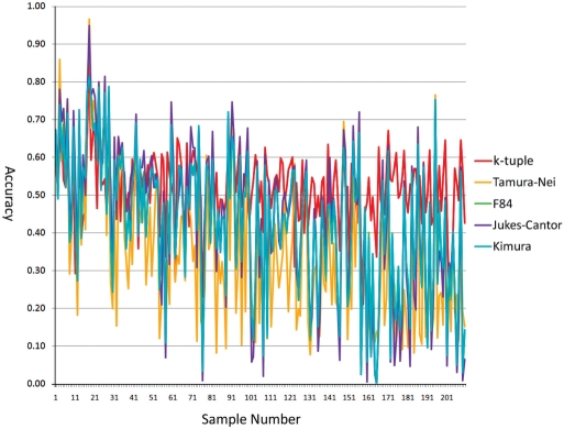
To see the performance of the k-tuple distance on real data, we obtained trees from the TreeFAM database. We used 210 trees together with their branch lengths as model trees to simulate dataset 2. Figure 2 shows the accuracies of all five distance estimators with the NJ method on dataset 2. Although the advantage of the k-tuple distance matrix is not as obvious as in dataset 1, we can see that k-tuple distance accuracy is above the other distance matrices most of the time. In fact, the k-tuple distance has the best performance for 127 of the 210 trees. Another very important advantage that is not very clearly shown in the figure is the stability of the k-tuple distance. It has a leading average accuracy of 0.51568 with the lowest standard deviation of 0.09604. Jukes–Cantor ranked second in terms of average accuracy (=0.43574) but has the highest standard deviation (=0.20702) among the five estimators. Kimura and F84 scored almost the same with an average accuracy of 0.42759 and 0.42550, respectively, and a standard deviation of 0.01831 and 0.18175, respectively. Tamura–Nei has the lowest average accuracy (0.35853) with a standard deviation of 0.19900. It is clear that, in additional to its high accuracy, the k-tuple distance also produced a much smaller standard deviation, which is an equally important factor in judging the performance of a metric. BioNJ trees gave a slightly better accuracy for all five estimators but the difference was very subtle (Table 2).

Figure 2.

The accuracy of all five metrics on dataset 2 with the NJ method.

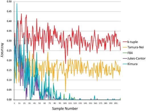
Figure 3 shows the performance comparison of five estimators on dataset 3 generated by random trees with sequence lengths from 500 to 1500 bp. It is interesting to note that as the number of taxa increases in the trees (the trees are arranged along the x-axis according to the ascending order of the number of taxa that trees contain), the accuracy of F84, Kimura and Juke–Cantor significantly dropped. Tamura–Nei and k-tuple distance maintained their accuracy regardless of the change of the number of taxa. As shown in Figure 3, after the 100th tree sample, which contained 150 taxa, F84, Jukes–Cantor and Kimura basically had the same performance as random clustering. The k-tuple distance achieved the highest average accuracy of 0.30889 with a standard deviation of 0.04278. Tamura–Nei had the second highest average accuracy of 0.16092 with a standard deviation of 0.03402. Kimura and F84 matrices performed similarly, with an average accuracy of 0.04410 and 0.04484, respectively, and a standard deviation of 0.08308 and 0.08374, respectively. Jukes–Cantor matrix ranked last with the lowest average accuracy of 0.03222 and a standard deviation of 0.07173.

Figure 3.

The accuracies of the five metrics on dataset 3 with the NJ method.

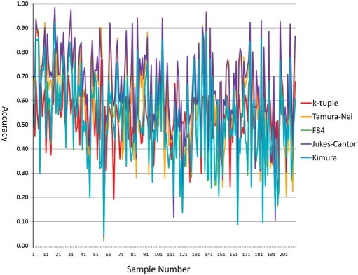
Figure 4 shows the comparison of accuracies of the metrics with the NJ method for dataset 4. Compared to results from other datasets, the accuracy difference decreased considerably, with the highest average accuracy of 0.64871 for Jukes–Cantor and the lowest 0.50200 for the F84 matrix. Tamura–Nei, k-tuple distance and Kimura ranked second, third and fourth with an average accuracy of 0.58316, 0.52836 and 0.50406, respectively. Despite the loss of advantage in accuracy, the k-tuple distance still maintained its leading position in terms of performance stability with the lowest standard deviation of 0.10363. The standard deviation for the Tamura–Nei, F84, Jukes–Cantor and Kimura matrices were 0.20987, 0.17209, 0.18384 and 0.17061, respectively. With BioNJ, we observed a better accuracy score for all five metrics, but the difference is trivial, <4% (Table 2).

Figure 4.

The accuracies of the five metrics on dataset 4 with the NJ method.

Figure 5 compares the accuracy of different distance matrices with the NJ method for dataset 5. With the increase of the number of taxa in the trees, the accuracy of F84, Jukes–Cantor and Kimura decreased greatly, similar to the observation in dataset 1 where sequences were simulated with indels using random trees. The k-tuple distance has the best performance followed by Tamura–Nei. In this dataset, BioNJ performed at almost the same level as traditional NJ (Table 2).

Figure 5.

The accuracies of the five metrics on dataset 5 with the NJ method.

Table 2 shows a summary of the average accuracy (A) and standard deviation (S) of the 50 combinations of the five distance estimators, five datasets and two tree-building methods. k-tuple distance outperformed other distance metrics in most cases. Its performance is very stable, as indicated by the low standard deviation. Only Tamura–Nei achieved a slightly lower standard deviation with the NJ method on dataset 5, which might be because the HKY model used to simulate sequence evolution is a special case of the Tamura–Nei model.

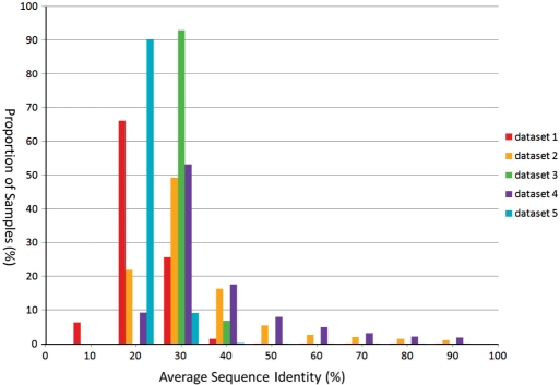
In order to examine the reason for the difference in accuracies of the k-tuple distance in the above datasets, we calculated the average pairwise sequence identity for each simulated sample. The distribution in each dataset is shown in Figure 6. The average pairwise sequence identity ranges from 8.53 to 79.43 in dataset 1, from 27.52 to 73.14 in dataset 2, from 26.07 to 31.15 in dataset 3, from 27.44 to 79.43 in dataset 4 and from 26.35 to 32.77 in dataset 5. Therefore, in general, the 210 sets of sequences in datasets 2 and 4 (generated from real trees) tend to have a higher average pairwise sequence identity than that of those in datasets 3 and 5 (generated from random trees).

Figure 6.

The distribution of average pairwise sequence identity in all the datasets.

DISCUSSION

In most cases, the performance of distance matrices is largely related to the size of the tree (i.e. the number of taxa in the tree), the length difference and the divergence of the sequences. Most distance matrices would produce good results with a small number of sequences of low divergence. However, as the number of sequences increases and sequence divergence increases, the accuracy measured by the symmetric difference will drop greatly for the alignment-dependent distance estimators.

The most significant difference between the accuracy of the k-tuple distance and the other distance estimators was found in dataset 1, which contains short sequences with high diversity. This dataset was generated to take account of upstream regulatory regions and short intronic sequences. Our results show that with the increase of sequence diversity and the number of taxa, the accuracy of all other matrices except the k-tuple distance has dropped tremendously (Figure 1). The decrease of accuracy is most likely due to decreased quality of MSAs. A recent study (5) on MSA algorithm performance has shown that all MSA programs return alignments of low accuracy when highly diverged sequences are used. This fact may explain the existence of the performance gap between the k-tuple distance, which does not rely on multiple sequence alignment to determine sequence distance, and the other distance estimators.

The most common scenario in phylogenetic tree reconstruction is to construct a tree from a group of sequences with different lengths from different species. Datasets 2 and 3 were generated to take account of this aspect. Difference in sequence lengths is introduced through indel rate setting in the sequence generation program and branch length in the model trees. The difference between real trees and randomly generated trees lies mostly on the branch lengths (i.e. the degree of sequence divergence). Specifically, real trees in TreeFAM are built mostly because sequence alignments are of high quality, which essentially limits the real trees to datasets containing only sequences that can be aligned by alignment programs. Due to this limitation, some remote gene family members might have been discarded from final alignments and therefore not considered in the trees. Random trees with long branch lengths can be used to compensate for this limitation.

When a set of sequences is highly diverged, the accuracy of the constructed phylogenetic trees is in general low regardless of the type of distance estimators used. Even though the k-tuple distance has the best performance in these cases, it is only about 30–40% accurate on average (e.g. Figures 1 and 3). F84, Jukes–Cantor and Kimura distances basically show performance similar to random clustering, especially when simulated samples contain >180 sequences (after sample #130 in Figures 1 and 3). The low performance of these distance estimators could be partially explained by the low accuracy of the MSAs. However, the fact that Tamura–Nei distances show a stronger accuracy and stability under such circumstances indicates that the simpler distance estimators, as compared to Tamura–Nei, is not a good fit to the underlying sequences, which were generated under the HKY model, a special case of the Tamura–Nei model (25). The observation is consistent with previous studies showing that choosing the right nucleotide substitution models are essential for correct phylogenetic analyses (26,27). In fact, when using the distance-based phylogenetic tree reconstruction, it has been suggested that statistical tests should be performed in order to choose the right substitution model for the underlying sequence alignments to calculate the distance matrix (28).

We also considered the evolution of DNA sequences without indels. As both insertion and deletion occur in DNA sequences, DNA sequences generated without indels are likely unrealistic, and this scenario may happen only to sequences that diverged from each other recently or to sequences that are under intensive purifying selection against indels. Due to the absence of indels in the sequences, under a suitable scoring scheme, an MSA can be constructed with few errors and little deviation from the true evolution of the sequences. An accurate MSA gives the most advantage to the alignment-dependent distance estimators. Therefore, this scenario can provide us the lower bound of the advantage of the k-tuple distance over other distance estimators. Our result shows that with similar sequences, the difference between different methods diminishes and the difference of the stability for the underlying metrics also decreases, although the k-tuple distance still shows 50% more stability than the others (Figure 4).

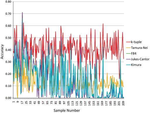
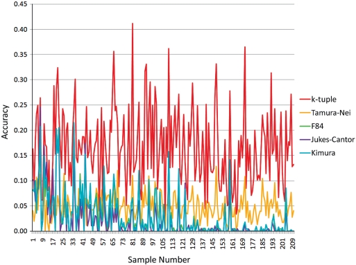
Clearly, alignment-based distances will have advantage over k-tuple distances in terms of tree accuracy in cases where k-tuple distances cannot reflect the degree of sequence divergence faithfully while alignment methods can. One of the extreme cases is when a set of sequences are almost identical, in which case, the k-tuple distance may have lower resolution than the more refined model-based distances, because, for example, it cannot differentiate transitions from transversions. However, a large number of highly identical sequences happens mostly in the studies of population genetics, in the majority of other cases, the large number of sequences that require phylogenetic tree reconstruction might have a wide range of sequence divergence, similar to what we observe in the dataset 2. Another extreme case is when rates of insertions and deletions are high and rates of point mutations are low. Conceivably, k-tuple distance could perform worse than alignment distance here. To formally investigate this, we simulated two more datasets using real trees and a different indel/substitution rate ratio scheme: the first dataset has a ratio of indel rates versus substitution rates of 1 and the second dataset has a ratio of indel rates versus substitution rates of 10 (Table 1). Previous studies show that the ratio of indel versus substitution rates is about 0.1 (29,30), and therefore, both the ratios of 1 and 10 are biologically unrealistic. Nevertheless, it is useful to see in these extreme cases the performance of the k-tuple distance as compared to that of other model-based distances. Results show that high rate ratios of indels versus substitutions harm the alignment-based methods more than k-tuple distance. While the average accuracy of the latter drops to from 0.53 (Figure 4) to 0.52 (Figure 2) to 0.41 and 0.17 (Figures 7 and 8) as the ratio increases from 0, 0.1, 1, to 10, respectively, the alignment based methods uniformly suffer a more catastrophic loss of performance. This result is a clear manifestation of the greater disruption by indels of alignment scores than of k-tuple distances.

Figure 7.

Accuracy comparison for dataset 6 with indel versus substitution rate ratio of 1.

Figure 8.

Accuracy comparison for dataset 7 with indel versus substitution rate ratio of 10.

To understand the impact of GC bias on the performance of k-tuple distance, we used real trees from TreeFam and indel/substitution rates of 0.1 and generated 150 sets of sequences that have different degrees of GC bias: 50 sets of sequences with strong GC bias (i.e. average GC content = 70%), 50 sets with little GC bias (i.e. average GC content = 50%) and 50 sets of AT rich (i.e. average GC content = 30%). Comparison of k-tuple trees with the model trees shows that the average accuracy of k-tuple trees is 53.84% (standard deviation = 0.11) in the no-GC-bias sequence sets, 48.76% (standard deviation = 0.09) in the strong-GC-bias sets and 48.65% (standard deviation = 0.09) in the AT-rich sets. This result suggests that base composition can affect the performance of k-tuple distance, although the impact seems small.

As simulation cannot capture all the complexities of real sequence evolution, it will be useful to perform some analyses on real data. However, real sequences with ‘real’ trees are not usually available. But it is still useful to examine how consistent k-tuple distance performs in building phylogenetic trees with the alignment-based distances and also how robust the k-tuple distance is as compared to the bootstrapped alignment-based trees. Bootstrapping is a common way to determine the quality and confidence of a reconstructed phylogenetic tree. It is usually done by re-sampling the sequences with replacement, repeating the tree-reconstruction processes for a certain number of times, and obtaining bootstrap values as the percentage times that certain bifurcation is supported by the reconstructed trees. Thus, bootstrapping gives confidence estimate of certain groupings in a phylogenetic tree. One would expect that highly supported phylogenetic groupings (i.e. having high bootstrap values) can be recovered by the trees produced by the k-tuple distance. To address these issues, we manually picked 10 genes from the TreeFam database to study whether the k-tuple distance can produce trees that agree with the alignment-based methods and whether the k-tuple trees can recover the highly supported phylogenetic groupings in the bootstrapped trees. We visually inspected all the k-tuple trees and alignment-based trees, and found that about 76% of the bifurcations that have bootstrapping values higher than 75% were recovered also by the k-tuple trees, whereas only 25% of the bifurcations that have bootstrap values lower than 30% were recovered. This indicates that the k-tuple trees have little difficulty in recovering the phylogenetic groupings that have high bootstrap confidence in the alignment-based trees, but for the phylogenetic groupings with low confidence in the alignment-based trees, k-tuple methods may also produce ambiguous grouping, similar to what happens to the alignment-based methods.

Broadly, the k-tuple distance falls into the category of alignment-free sequence comparison metrics. Except the k-tuple distance used in this study, there are other more elaborated ones that are also based on tuple frequencies, such as the Mahalanobis distance and Weighted Enclidean distance (31). Some of these alignment-free distance measurements have been previously explored in the application of searching DNA and protein databases. Though there is no evidence yet that any of these are preferable to simple k-tuple distance, this is a likely question for further research.

Compared to the most popular ClustalW program, MUSCLE gives accurate alignments faster. ClustalW becomes impractical when the lengths and number of sequences increase to certain extent. However, even though MUSCLE is faster than ClustalW, it on average still takes 30–40 min to align 250 sequences of around 1300 bp. In contrast, it takes only seconds to calculate the k-tuple distance matrix. Therefore, the advantage of the k-tuple distance over existing distance estimators in distance-based phylogenetic tree reconstruction is not only its accuracy, but also its computational speed: it is at least hundreds of times, if not thousands, faster than any other distance estimators that require an MSA to calculate distances between sequences. It can be very useful in constructing phylogenetic trees for a large number of sequences, for example, in the case of building the ‘tree of life’ (32,33).

REFERENCES

- 1.Jin G, Nakhleh L, Snir S, Tuller T. Efficient parsimony-based methods for phylogenetic network reconstruction. Bioinformatics. 2007;23:e123–e128. doi: 10.1093/bioinformatics/btl313. [DOI] [PubMed] [Google Scholar]
- 2.Saitou N, Nei M. The neighbor-joining method: a new method for reconstructing phylogenetic trees. Mol. Biol. Evol. 1987;4:406–425. doi: 10.1093/oxfordjournals.molbev.a040454. [DOI] [PubMed] [Google Scholar]
- 3.Gascuel O. BIONJ: an improved version of the NJ algorithm based on a simple model of sequence data. Mol. Biol. Evol. 1997;14:685–695. doi: 10.1093/oxfordjournals.molbev.a025808. [DOI] [PubMed] [Google Scholar]
- 4.Bruno WJ, Socci ND, Halpern AL. Weighted neighbor joining: a likelihood-based approach to distance-based phylogeny reconstruction. Mol. Biol. Evol. 2000;17:189–197. doi: 10.1093/oxfordjournals.molbev.a026231. [DOI] [PubMed] [Google Scholar]
- 5.Blackshields G, Wallace IM, Larkin M, Higgins DG. Analysis and comparison of benchmarks for multiple sequence alignment. In Silico Biol. 2006;6:321–339. [PubMed] [Google Scholar]
- 6.Wallance IM, O'Sullivan O, Higgins DG, Notredame C. M-Coffee: combining multiple sequence alignment methods with T-Coffee. Nucleic Acids Res. 2006;34:7. doi: 10.1093/nar/gkl091. [DOI] [PMC free article] [PubMed] [Google Scholar]
- 7.Chenna R, Sugawara H, Koike T, Lopez R, Gibson TJ, Higgins DG, Thompson JD. Multiple sequence alignment with the Clustal series of programs. Nucleic Acids Res. 2003;31:4. doi: 10.1093/nar/gkg500. [DOI] [PMC free article] [PubMed] [Google Scholar]
- 8.Notredame C, Higgins DG, Heringa J. T-Coffee: a novel method for fast and accurate multiple sequence alignment. J. Mol. Biol. 2000;302:13. doi: 10.1006/jmbi.2000.4042. [DOI] [PubMed] [Google Scholar]
- 9.Katoh K, Misawa K, Kuma K, Miyata T. MAFFT: a novel method for rapid multiple sequence alignment based on fast Fourier transform. Nucleic Acids Res. 2000;30:8. doi: 10.1093/nar/gkf436. [DOI] [PMC free article] [PubMed] [Google Scholar]
- 10.Edgar RC. MUSCLE: multiple sequence alignment with high accuracy and high throughput. Nucleic Acids Res. 2004;32:6. doi: 10.1093/nar/gkh340. [DOI] [PMC free article] [PubMed] [Google Scholar]
- 11.Lassmann T, Sonnhammer EL. Kalign–an accurate and fast multiple sequence alignment algorithm. BMC Bioinformatics. 2005;6:298. doi: 10.1186/1471-2105-6-298. [DOI] [PMC free article] [PubMed] [Google Scholar]
- 12.Felsenstein J. PHYLIP - Phylogeny Inference Package (Version 3.2) Cladistics. 1989;5:164–166. [Google Scholar]
- 13.Swofford DL. Sunderland, Massachusetts: Sinauer Associates; 2002. PAUP*. Phylogenetic Analysis Using Parsimony (*and Other Methods) [Google Scholar]
- 14.Cartwright RA. DNA assembly with gaps (Dawg): simulating sequence evolution. Bioinformatics. 2005;21(Suppl. 3):iii31–iii38. doi: 10.1093/bioinformatics/bti1200. [DOI] [PubMed] [Google Scholar]
- 15.Hasegawa M, Kishino H, Yano T. Dating of the human-ape splitting by a molecular clock of mitochondrial DNA. J. Mol. Evol. 1985;22:160–174. doi: 10.1007/BF02101694. [DOI] [PubMed] [Google Scholar]
- 16.Li H, Coghlan A, Ruan J, Coin LJ, Heriche JK, Osmotherly L, Li R, Liu T, Zhang Z. TreeFam: a curated database of phylogenetic trees of animal gene families. Nucleic Acids Res. 2006;34:D572–D580. doi: 10.1093/nar/gkj118. [DOI] [PMC free article] [PubMed] [Google Scholar]
- 17.Karlin S, Burge C. Dinucleotide relative abundance extremes: a genomic signature. Trends Genet. 1995;11:283–290. doi: 10.1016/s0168-9525(00)89076-9. [DOI] [PubMed] [Google Scholar]
- 18.Karlin S. Global dinucleotide signatures and analysis of genomic heterogeneity. Curr. Opin. Microbiol. 1998;1:598–610. doi: 10.1016/s1369-5274(98)80095-7. [DOI] [PubMed] [Google Scholar]
- 19.Kishino H, Hasegawa M. Evaluation of the maximum likelihood estimate of the evolutionary tree topologies from DNA sequence data, and the branching order in Hominoidea. J. Mol. Evol. 1989;29:10. doi: 10.1007/BF02100115. [DOI] [PubMed] [Google Scholar]
- 20.Jukes TH, Cantor CR. Evolution of protein molecules. In: Munro HN, editor. Mammalian Protein Metabolism. 1969. Academic Press, New York, pp. 21–132. [Google Scholar]
- 21.Kimura M. A simple method for estimating evolutionary rates of base substitutions through comparative studies of nucleotide sequences. J. Mol. Evol. 1980;16:10. doi: 10.1007/BF01731581. [DOI] [PubMed] [Google Scholar]
- 22.Tamura K, Nei M. Estimation of the number of nucleotide substitutions in the control region of mitochondrial DNA in humans and chimpanzees. J. Mol. Evol. 1993;10:512–526. doi: 10.1093/oxfordjournals.molbev.a040023. [DOI] [PubMed] [Google Scholar]
- 23.Hollich V, Milchert L, Arvestad L, Sonnhammer EL. Assessment of protein distance measures and tree-building methods for phylogenetic tree reconstruction. J. Mol. Evol. 2005;22:2257–2264. doi: 10.1093/molbev/msi224. [DOI] [PubMed] [Google Scholar]
- 24.Penny D, Hendy MD. The use of tree comparison metrics. Syst. Zool. 1985;34:12. [Google Scholar]
- 25.Li W-H. Molecular Evolution. Sunderland, MA: Sinauer Associates; 1997. [Google Scholar]
- 26.Huelsenbeck JP, Larget B, Alfaro ME. Bayesian phylogenetic model selection using reversible jump Markov chain Monte Carlo. Mol. Biol. Evol. 2004;21:1123–1133. doi: 10.1093/molbev/msh123. [DOI] [PubMed] [Google Scholar]
- 27.Bos DH, Posada D. Using models of nucde evolution to leotibuild phylogenetic trees. Dev. Comp. Immunol. 2005;29:211–227. doi: 10.1016/j.dci.2004.07.007. [DOI] [PubMed] [Google Scholar]
- 28.Posada D. ModelTest Server: a web-based tool for the statistical selection of models of nucleotide substitution online. Nucleic Acids Res. 2006;34:W700–W703. doi: 10.1093/nar/gkl042. [DOI] [PMC free article] [PubMed] [Google Scholar]
- 29.Zhang Z, Gerstein M. Patterns of nucleotide substitution, insertion and deletion in the human genome inferred from pseudogenes. Nucleic Acids Res. 2003;31:5338–5348. doi: 10.1093/nar/gkg745. [DOI] [PMC free article] [PubMed] [Google Scholar]
- 30.Saitou N, Ueda S. Evolutionary rates of insertion and deletion in noncoding nucleotide sequences of primates. Mol. Biol. Evol. 1994;11:504–512. doi: 10.1093/oxfordjournals.molbev.a040130. [DOI] [PubMed] [Google Scholar]
- 31.Vinga S, Almeida J. Alignment-free sequence comparison-a review. Bioinformatics. 2003;19:513–523. doi: 10.1093/bioinformatics/btg005. [DOI] [PubMed] [Google Scholar]
- 32.Morrison DA. A review of: ‘the tree of life: a phylogenetic classification’. Syst. Biol. 2007;56:696–698. [Google Scholar]
- 33.Rokas A. Genomics. Genomics and the tree of life. Science (New York) 2006;313:1897–1899. doi: 10.1126/science.1134490. [DOI] [PubMed] [Google Scholar]