Characteristic temperatures of folding of a small peptide

Abstract

We perform a generalized-ensemble simulation of a small peptide taking the interactions among all atoms into account. From this simulation we obtain thermodynamic quantities over a wide range of temperatures. In particular, we show that the folding of a small peptide is a multistage process associated with two characteristic temperatures, the collapse temperature T_θ and the folding temperature T_ƒ. Our results give supporting evidence for the energy landscape picture and funnel concept. These ideas were previously developed in the context of studies of simplified protein models, and here are checked in an all-atom Monte Carlo simulation.

It is well known that a large class of proteins fold spontaneously into globular states of unique shape, yet the mechanism of folding has remained elusive. The folding process may be either thermodynamically or kinetically controlled. The thermodynamic hypothesis assumes that the folded state corresponds to the global minimum in free energy and is supported by the famous work of Anfinsen (1) and similar experiments. On the other hand, Levinthal (2) has argued that because of the huge number of local energy minima available to a protein it is impossible to find the global free energy minimum by a random search in biological time scales (of order seconds). His argument rather suggests that the protein folds into a unique metastable state, the kinetically most accessible structure. The complexity and importance of the problem raised a lot of interest in the subject over the last three decades, but no complete solution is in sight to date. However, significant new insight was gained over the last few years from the studies of minimal protein models. Both lattice models (3–15) and continuum models (16–22) have been extensively studied. Common to all these models is that they capture only a few, but probably dominant, interactions in real proteins. These include chain connectivity, excluded volume, hydrophobicity as the driving force, and sequence heterogeneity. For recent reviews on minimal protein models and their applications, see refs. 23–26. From the numerical and analytical studies of these models a different view of the folding process emerged. The folding kinetics is seen to be determined by an energy landscape that for foldable proteins resembles a funnel with a free energy gradient toward the native structure (8, 12, 13, 23, 25). The funnel is itself rough, and folding occurs by a multistage, multipathway kinetics. A common scenario for folding may be that first the polypeptide chain collapses from a random coil to a compact state. This coil-to-globular transition is characterized by the collapse transition temperature T_θ. In the second stage, a set of compact structures is explored. The final stage involves a transition from one of the many local minima in the set of compact structures to the native conformation. This final transition is characterized by the folding temperature T_ƒ (≤ T_θ). It was conjectured that the kinetic accessibility of the native conformation can be classified by the parameter (9,14)

1

i.e., the smaller σ is, the more easily a protein can fold. If T_θ ≈ T_ƒ (i.e., σ ≈ 0), the second stage will be very short or not exist, and the protein will fold in an all or nothing transition from the extended coil to the native conformation without any detectable intermediates. On the other hand, for some proteins the folding process may involve further stages. A more elaborate classification of possible folding processes is discussed in ref. 23.

One can ask whether the picture outlined above is really useful to describe the folding kinetics of real proteins, because the underlying models are gross simplifications of real protein systems. For instance, side-chain conformational degrees of freedom that are important for packing are neglected. The situation actually resembles a vicious circle. The energy landscape picture and the analogy to phase transitions were developed from studies of the highly simplified description of proteins by minimal models. However, only if these concepts apply for proteins is it possible to argue that the broad mechanism of phase transitions depends solely on gross features of the energy function, not on their details. Only in this case a law of corresponding states can be applied to explain dynamics of real proteins from studies of the folding kinetics in minimal models. It therefore is desirable to check the above picture by comparison with more realistic energy functions, namely with all-atom simulations of a suitable protein. This is the purpose of this article. Although an attempt has been made to study the free energy landscape of an all-atom protein model by unfolding molecular dynamics simulations (27), the present work starts from random initial conformations and rather is concerned with obtaining characteristic temperatures of protein folding by a Monte Carlo simulation (and thus studying the energy landscape indirectly).

Simulations of proteins where the interactions among all atoms are taken into account have been notoriously difficult (for a recent review, see ref. 28). The various competing interactions yield to a much rougher energy landscape than for minimal protein models. (In fact, one might question whether the limitations of the current energy functions may lead to rougher energy landscapes than the protein encounters in nature.) Simulations based on canonical Monte Carlo or molecular dynamics techniques will, at low temperatures, get trapped in one of the multitude of local minima separated by high energy barriers. Hence, only small parts of configuration space are sampled, and physical quantities cannot be calculated accurately. However, with the development of generalized-ensemble techniques like multicanonical algorithms (29) and simulated tempering (30, 31), an efficient sampling of low-energy configurations and calculation of accurate low-temperature thermodynamic quantities became feasible. The first application of one of these techniques to the protein folding problem can be found in ref. 32. Later applications of multicanonical algorithms include the study of the coil-globular transitions of a simplified model protein (11) and the helix-coil transitions of homo-oligomers of nonpolar amino acids (33). A formulation of multicanonical algorithm for the molecular dynamics method also was developed (34, 35). A numerical comparison of three different generalized-ensemble algorithms can be found in ref. 36.

The generalized-ensemble technique we use in this article was first introduced in refs. 37 and 38 and is related to Tsallis generalized mechanics formalism (39). In this algorithm, configurations are updated according to the following probability weight:

2

where E₀ is an estimator for the ground-state energy, n_F is the number of degrees of freedom of the system, and β = 1/k_BT is the inverse temperature with a low temperature T (and k_B is the Boltzmann constant). Obviously, the new weight reduces in the low-energy region to the canonical Boltzmann weight exp(−βE) for β(E−E₀)/n_F ≪ 1. On the other hand, high-energy regions are no longer exponentially suppressed but only according to a power law, which enhances excursions to high-energy regions. In contrast to other generalized-ensemble techniques where the determination of weights is nontrivial, the weight of the new ensemble is explicitly given by Eq. 2. One only needs to find an estimator for the ground-state energy E₀, which can be done by a procedure described in ref. 38, and is much easier than the determination of weights for other generalized ensembles. Because the simulation by the present algorithm samples a large range of energies, we can use the reweighting techniques (40) to construct canonical distributions and calculate thermodynamic average of any physical quantity 𝒜 over a wide temperature range:

3

where x stands for configurations.

Here, we use these techniques to examine the picture for the folding kinetics as proposed from the simulations of minimal models. Limitations in available computational time force us to restrict ourselves on the simulation of small molecules, and we have, in addition, neglected explicit solvent interactions. The system of our choice is Met-enkephalin, one of the simplest peptides, with which we are familiar from earlier work (32, 36, 41). Met-enkephalin has the amino acid sequence Tyr-Gly-Gly-Phe-Met. The potential energy function E_tot (in kcal/mol) that we used is given by the sum of the electrostatic term E_es, 12–6 Lennard–Jones term E_LJ, and hydrogen-bond term E_hb for all pairs of atoms in the peptide together with the torsion term E_tors for all torsion angles:

4

5

6

7

8

where r_ij (in Å) is the distance between the atoms i and j, and χ_l is the l-th torsion angle. The parameters (q_i, A_ij, B_ij, C_ij, D_ij, U_l, and n_l) for the energy function were adopted from ECEPP/2 (45). The dielectric constant ɛ was set equal to 2. In ECEPP/2 bond lengths and bond angles are fixed at experimental values. We further fix the peptide bond angles ω to their common value 180°, which leaves us with 19 torsion angles (φ, ψ, and χ) as independent degrees of freedom (i.e., n_F = 19). The computer code KONF90 (46, 47) was used. We remark that KONF90 uses a different convention for the implementation of the ECEPP parameters (for example, φ₁ of ECEPP/2 is equal to φ₁ − 180° of KONF90). Therefore, our energy values are slightly different from those of the original implementation of ECEPP/2. The simulation was started from a completely random initial conformation (Hot Start). One Monte Carlo sweep updates every torsion angle of the peptide once.

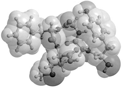
It is known from our previous work that the ground-state conformation for Met-enkephalin has the KONF90 energy value E_GS = −12.2 kcal/mol (41). We therefore set E₀ = −12.2 kcal/mol and T = 50 K (or, β = 10.1 [1/kcal/mol]) (and n_F = 19) in our probability weight factor in Eq. 2. The ground-state structure, exhibiting a II′-type β turn, is shown in Fig. 1. It is a superposition of ball-and-stick and space-filling representations. The latter representation was added to give a rough idea of the volume of the peptide as discussed below.

Figure 1.

Ground-state conformation of Met-enkephalin for KONF90 energy function. The figure was created with molscript (42) and raster3d (43, 44).

All thermodynamic quantities then were calculated from a single production run of 1,000,000 Monte Carlo sweeps, which followed 10,000 sweeps for thermalization. At the end of every fourth sweep we stored the energies of the conformation, the corresponding volume, and the overlap of the conformation with the (known) ground state for further analyses. Here, we approximate the volume of the peptide by its solvent excluded volume (in ų), which is calculated by a variant (the program for calculation of solvent-excluded volume was written by M.M. and will be described in detail elsewhere) of the double cubic lattice method (48). Our definition of the overlap, which measures how much a given conformation differs from the ground state, is given by

9

where α_i^(t) and α_j^(GS) (in degrees) stand for the n_F dihedral angles of the conformation at t-th Monte Carlo sweep and the ground-state conformation, respectively. Symmetries for the side-chain angles were taken into account and the difference α_i^(t) − α_i^(GS) always was projected into the interval [−180°, 180°]. Our definition guarantees that we have

10

with the limiting values

11

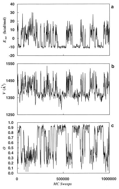
Let us now present our results. In Fig. 2a we show the time series of the total potential energy E_tot. It is a random walk in potential energy space, which keeps the simulation from getting trapped in a local minimum. It indeed visits the low-energy region several times in 1,000,000 Monte Carlo sweeps. The visits are separated by excursions into high-energy regions, which ensures de-correlation of the configurations. This can be seen in Fig. 2 b and c, where time series of the excluded volume and the overlap function are displayed. The large changes in these quantities imply the large conformational changes that happen in the course of the simulation. Because large parts of the configuration space are sampled, the use of the reweighting techniques (40) is justified to calculate thermodynamic quantities over a wide range of temperatures by Eq. 3.

Figure 2.

Time series of total potential energy E_tot (kcal/mol) (a), volume V (ų) (b), and overlap O (defined by Eq. 9) (c) as obtained by a generalized-ensemble simulation of 1,000,000 Monte Carlo sweeps.

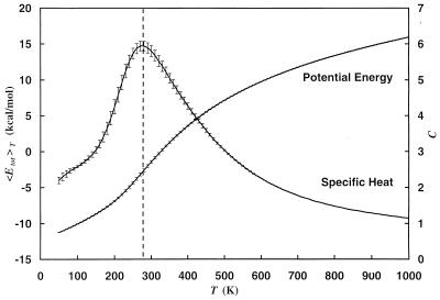
We expect the folding of proteins and peptides to occur in a multistage process. The first process is connected with a collapse of the extended coil structure into an ensemble of compact structures. This transition should be connected with a pronounced change in the average potential energy as a function of temperature. At the transition temperature we therefore expect a peak in the specific heat. Both quantities are shown in Fig. 3. We clearly observe a steep decrease in total potential energy around 300 K and the corresponding peak in the specific heat defined by

12

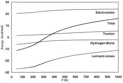
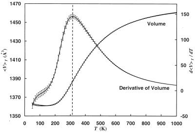
where N (= 5) is the number of amino acid residues in the peptide. In Fig. 4 we display the average values of each of the component terms of the potential energy (defined in Eqs. 5–8) as a function of temperature. As one can see in the figure, the change in average potential energy is mainly caused by the Lennard–Jones term and therefore is connected to a decrease of the volume occupied by the peptide. This can be seen in Fig. 5, where we display the average volume as a function of temperature. As expected, the volume decreases rapidly in the same temperature range as the potential energy. The average volume is a natural measure of compactness, but the change from extended coil structures to compact structures with decreasing temperature also can be observed in other quantities like the average end-to-end distance 〈d_e−e〉_T (here, defined to be the distance between N of Tyr¹ and O of Met⁵). In Table 1, we give some of the values of 〈d_e−e〉_T as a function of temperature. The results imply again that the peptide is quite extended at high temperatures and compact at low temperatures.

Figure 3.

Average total potential energy 〈E_tot〉_T and specific heat C as a function of temperature. The dotted vertical line is added to aid the eyes in locating the peak of specific heat. The results were obtained from a generalized-ensemble simulation of 1,000,000 Monte Carlo sweeps.

Figure 4.

Average potential energies as a function of temperature. The results were obtained from a generalized-ensemble simulation of 1,000,000 Monte Carlo sweeps.

Figure 5.

Average volume 〈V〉_T and its derivative d〈V〉_T/dT as a function of temperature. The dotted vertical line is added to aid the eyes in locating the peak of the derivative of volume. The results were obtained from a generalized-ensemble simulation of 1,000,000 Monte Carlo sweeps.

Table 1.

Average end-to-end distance 〈d_e−e〉_T (Å) of Met-enkephalin as a function of temperature T (K)

T	50	100	150	200	250	300	400	700	1,000
〈de−e〉T	4.8	4.8	4.9	5.2	5.8	6.8	8.6	11.0	11.5

If both energy and volume decrease are correlated, then the transition temperature T_θ can be located both from the position where the specific heat has its maximum and from the position of the maximum of

13

which also is displayed in Fig. 5. The second quantity measures the steepness of the decrease in volume in the same way as the specific heat measures the steepness of decrease of potential energy. To quantify its value we divided our time series in four bins corresponding to 250,000 sweeps each, determined the position of the maximum for both quantities in each bin and averaged over the bins. In this way we found a transition temperature T_θ = 280 ± 20 K from the location of the peak in specific heat and T_θ = 310 ± 20 K from the maximum in d〈V〉_T/dT. Both temperatures are indeed consistent with each other within the error bars.

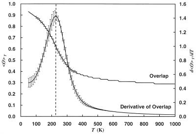
The second transition that should occur at a lower temperature T_ƒ is that from a set of compact structures to the native conformation that is considered to be the ground state of the peptide. Because these compact conformations are expected to be all of similar volume and energy (systematic comparisons of such structures were tried in previous work; refs. 49–51), we do not expect to see this transition by pronounced changes in 〈E_tot〉_T or to find another peak in the specific heat. Instead this transition should be characterized by a rapid change in the average overlap 〈O〉_T with the ground-state conformation (see Eq. 9) and a corresponding maximum in

14

Both quantities are displayed in Fig. 6, and we indeed find the expected behavior. The change in the order parameter is clearly visible and occurs at a temperature lower than the first transition temperature T_θ. We again try to determine its value by searching for the peak in d〈O〉_T/dT in each of the four bins and averaging over the obtained values. In this way we find a transition temperature of T_ƒ = 230 ± 30 K. We remark that the average overlap 〈O〉_T approaches its limiting value zero only very slowly as the temperature increases. This is because 〈O〉_T = 0 corresponds to a completely random distribution of dihedral angles, which is energetically highly unfavorable because of the steric hindrance of both main and side chains.

Figure 6.

Average overlap 〈O〉_T and the absolute value of its derivative d〈O〉_T/dT as a function of temperature. The dotted vertical line is added to aid the eyes in locating the peak of the derivative of overlap. The results were obtained from a generalized-ensemble simulation of 1,000,000 Monte Carlo sweeps.

One characterization of the folding properties of a peptide or protein is given by the parameter σ of Eq. 1. With our values for T_θ and T_ƒ, we have for Met-enkephalin σ ≈ 0.2. Here, we have taken the central values: T_θ = 295 K and T_ƒ = 230 K. This value of σ implies that our peptide has reasonably good folding properties according to refs. 9 and 14. We remark that the characterization of Met-enkephalin as a good folder has to be taken with care: Low-temperature simulations of the molecules with conventional methods are still a formidable task and a low value of σ may not necessarily indicate easy foldability in a computer simulation.

Although the collapse temperature T_θ is roughly equal to room temperature, the transition temperature T_ƒ is well below room temperature. Consequently, contributions of ground-state conformers are not dominant at room temperature for Met-enkephalin, as was observed in our earlier work (32, 41). This is due to the small size of the peptide. However, it still can be regarded as a good model for a small protein, because it has a unique stable structure below T_ƒ. It was shown in refs. 32 and 41 that Met-enkephalin remains mainly in the vicinity of the ground state without getting trapped in any of the local-minimum structures below T_ƒ (≈230 K).

We also performed a generalized-ensemble simulation with the same statistics for a second peptide, Leu-enkephalin (data not shown). We found: T_θ = 300 ± 30 K and T_ƒ = 220 ± 30 K. These transition temperatures are essentially the same as for Met-enkephalin. Both peptides are very similar, differing only in the side chains of the Met (Leu) residue. Our results indicate that indeed the general mechanism of the transition does not depend on these details and a law of corresponding state can be applied for similar peptides.

Let us summarize our results. We have performed a generalized-ensemble simulation of a small peptide taking the interactions among all atoms into account and calculated thermodynamic averages of physical quantities over a wide range of temperatures. We found for this peptide two characteristic temperatures. The higher temperature is associated with a collapse of the peptide from extended coils into more compact structures, whereas the second one indicates the transition between an ensemble of compact structures and a phase that is dominated by a single conformation, the ground state of the peptide. Our results support pictures for the kinetics of protein folding, which were developed from the study, both numerical and analytical, of simplified protein models. It is still an open question whether these minimal models can be used for predictions of protein conformations. However, our analyses, performed with an energy function that takes much more of the details of a protein into account, demonstrate that these models are indeed able to describe the general mechanism of the folding process. Hence, the study of simplified models may in this way guide further simulations with more realistic energy functions. The present paper aims to be a step in this direction.

References

- 1.Anfinsen C B. Science. 1973;181:223–230. doi: 10.1126/science.181.4096.223. [DOI] [PubMed] [Google Scholar]
- 2.Levinthal C. J Chem Phys. 1968;65:44–45. [Google Scholar]
- 3.Taketomi H, Ueda Y, Gō N. Int J Pept Protein Res. 1975;7:445–459. [PubMed] [Google Scholar]
- 4.Skolnik J, Kolinski A. Science. 1990;250:1121–1125. doi: 10.1126/science.250.4984.1121. [DOI] [PubMed] [Google Scholar]
- 5.Chan H S, Dill K A. Annu Rev Biophys Biophys Chem. 1991;20:447–490. doi: 10.1146/annurev.bb.20.060191.002311. [DOI] [PubMed] [Google Scholar]
- 6.Shakhnovitch E I, Farztdinov G M, Gutin A M, Karplus M. Phys Rev Lett. 1991;67:1665–1668. doi: 10.1103/PhysRevLett.67.1665. [DOI] [PubMed] [Google Scholar]
- 7.Miller R, Danko C A, Fasolka M J, Balazs A C, Chan H S, Dill K A. J Chem Phys. 1992;96:768–780. [Google Scholar]
- 8.Leopold P E, Montal M, Onuchic J N. Proc Natl Acad Sci USA. 1992;89:8721–8725. doi: 10.1073/pnas.89.18.8721. [DOI] [PMC free article] [PubMed] [Google Scholar]
- 9.Camacho C J, Thirumalai D. Proc Natl Acad Sci USA. 1993;90:6369–6372. doi: 10.1073/pnas.90.13.6369. [DOI] [PMC free article] [PubMed] [Google Scholar]
- 10.Sali A, Shakhnovitch E I, Karplus M. J Mol Biol. 1994;235:1614–1636. doi: 10.1006/jmbi.1994.1110. [DOI] [PubMed] [Google Scholar]
- 11.Hao M-H, Scheraga H A. J Phys Chem. 1994;98:4940–4948. [Google Scholar]
- 12.Onuchic J N, Wolynes P G, Luthey-Schulten Z, Socci N D. Proc Natl Acad Sci USA. 1995;92:3626–3630. doi: 10.1073/pnas.92.8.3626. [DOI] [PMC free article] [PubMed] [Google Scholar]
- 13.Socci N D, Onuchic J N, Wolynes P G. J Chem Phys. 1996;104:5860–5871. [Google Scholar]
- 14.Klimov D K, Thirumalai D. Phys Rev Lett. 1996;76:4070–4073. doi: 10.1103/PhysRevLett.76.4070. [DOI] [PubMed] [Google Scholar]
- 15.Kolinski A, Galazka W, Skolnik J. Proteins. 1996;26:271–287. doi: 10.1002/(SICI)1097-0134(199611)26:3<271::AID-PROT4>3.0.CO;2-H. [DOI] [PubMed] [Google Scholar]
- 16.Levitt M, Warshel A. Nature (London) 1975;253:694–698. doi: 10.1038/253694a0. [DOI] [PubMed] [Google Scholar]
- 17.Bryngelson J D, Wolynes P G. Proc Natl Acad Sci USA. 1987;84:7524–7528. doi: 10.1073/pnas.84.21.7524. [DOI] [PMC free article] [PubMed] [Google Scholar]
- 18.Bryngelson J D, Wolynes P G. J Phys Chem. 1989;93:6902–6915. [Google Scholar]
- 19.Bryngelson J D, Wolynes P G. Biopolymers. 1990;30:177–188. [Google Scholar]
- 20.Honeycutt J D, Thirumalai D. Proc Natl Acad Sci USA. 1990;87:3526–3529. doi: 10.1073/pnas.87.9.3526. [DOI] [PMC free article] [PubMed] [Google Scholar]
- 21.Sasai M, Wolynes P G. Phys Rev A. 1992;46:7979–7997. doi: 10.1103/physreva.46.7979. [DOI] [PubMed] [Google Scholar]
- 22.Fukugita M, Lancaster D, Mitchard M G. Biopolymers. 1997;41:239–250. [Google Scholar]
- 23.Bryngelson J D, Onuchic J N, Socci N D, Wolynes P G. Proteins. 1995;21:167–195. doi: 10.1002/prot.340210302. [DOI] [PubMed] [Google Scholar]
- 24.Karplus M, Sali M. Curr Opin Struct Biol. 1995;5:58–73. doi: 10.1016/0959-440x(95)80010-x. [DOI] [PubMed] [Google Scholar]
- 25.Dill K A, Chan H S. Nat Struct Biol. 1997;4:10–19. doi: 10.1038/nsb0197-10. [DOI] [PubMed] [Google Scholar]
- 26.Shakhnovitch E I. Curr Opin Struct Biol. 1997;7:29–40. doi: 10.1016/s0959-440x(97)80005-x. [DOI] [PubMed] [Google Scholar]
- 27.Boczko E M, Brooks C L., III Science. 1995;269:393–396. doi: 10.1126/science.7618103. [DOI] [PubMed] [Google Scholar]
- 28.Vásquez M, Némethy G, Scheraga H A. Chem Rev. 1994;94:2183–2239. [Google Scholar]
- 29.Berg B A, Neuhaus T. Phys Lett B. 1991;267:249–253. [Google Scholar]
- 30.Lyubartsev A P, Martinovski A A, Shevkunov S V, Vorontsov-Velyaminov P N. J Chem Phys. 1992;96:1776–1783. [Google Scholar]
- 31.Marinari E, Parisi G. Europhys Lett. 1992;19:451–458. [Google Scholar]
- 32.Hansmann U H E, Okamoto Y. J Comp Chem. 1993;14:1333–1338. [Google Scholar]
- 33.Okamoto Y, Hansmann U H E. J Phys Chem. 1995;99:11276–11287. [Google Scholar]
- 34.Hansmann U H E, Okamoto Y, Eisenmenger F. Chem Phys Lett. 1996;259:321–330. [Google Scholar]
- 35.Nakajima N, Nakamura H, Kidera A. J Phys Chem. 1997;101:817–824. [Google Scholar]
- 36.Hansmann U H E, Okamoto Y. J Comp Chem. 1997;18:920–933. [Google Scholar]
- 37.Hansmann, U. H. E. (1997) Physica A, in press.
- 38.Hansmann U H E, Okamoto Y. Phys Rev E. 1997;56:2228–2233. [Google Scholar]
- 39.Tsallis C. J Stat Phys. 1988;52:479–487. [Google Scholar]
- 40.Ferrenberg A M, Swendsen R H. Phys Rev Lett. 1988;61:2635–2638. doi: 10.1103/PhysRevLett.61.2635. , and erratum (1989) 63, 1658. [DOI] [PubMed] [Google Scholar]
- 41.Hansmann U H E, Okamoto Y. Physica A. 1994;212:415–437. [Google Scholar]
- 42.Kraulis P J. J Appl Crystallogr. 1991;24:946–950. [Google Scholar]
- 43.Bacon D, Anderson W F. J Mol Graphics. 1988;6:219–220. [Google Scholar]
- 44.Merritt E A, Murphy M E P. Acta Crystallogr D. 1994;50:869–873. doi: 10.1107/S0907444994006396. [DOI] [PubMed] [Google Scholar]
- 45.Sippl M J, Némethy G, Scheraga H A. J Phys Chem. 1984;88:6231–6233. [Google Scholar]
- 46.Kawai H, Okamoto Y, Fukugita M, Nakazawa T, Kikuchi T. Chem Lett. 1991;1991:213–216. [Google Scholar]
- 47.Okamoto Y, Fukugita M, Nakazawa T, Kawai H. Protein Eng. 1991;4:639–647. doi: 10.1093/protein/4.6.639. [DOI] [PubMed] [Google Scholar]
- 48.Eisenhaber F, Lijnzaad P, Argos P, Sander C, Scharf M. J Comp Chem. 1995;16:273–284. [Google Scholar]
- 49.Freyberg B, von Braun W. J Comp Chem. 1991;12:1065–1076. [Google Scholar]
- 50.Okamoto Y, Kikuchi T, Kawai H. Chem Lett. 1992;1992:1275–1278. [Google Scholar]
- 51.Eisenmenger F, Hansmann U H E. J Phys Chem B. 1997;101:3304–3310. [Google Scholar]