How common is the funnel-like energy landscape in protein-protein interactions?

Abstract

The goal of this study is to verify the concept of the funnel-like intermolecular energy landscape in protein–protein interactions by use of a series of computational experiments. Our preliminary analysis revealed the existence of the funnel in many protein–protein interactions. However, because of the uncertainties in the modeling of these interactions and the ambiguity of the analysis procedures, the detection of the funnels requires detailed quantitative approaches to the energy landscape analysis. A number of such approaches are presented in this study. We show that the funnel detection problem is equivalent to a problem of distinguishing between distributions of low-energy intermolecular matches in the funnel and in the low-frequency landscape fluctuations. If the fluctuations are random, the decision about whether the minimum is the funnel is equivalent to determining whether this minimum is significantly different from a would-be random one. A database of 475 nonredundant cocrystallized protein–protein complexes was used to re-dock the proteins by use of smoothed potentials. To detect the funnel, we developed a set of sophisticated models of random matches. The funnel was considered detected if the binding area was more populated by the low-energy docking predictions than by the matches generated in the random models. The number of funnels detected by use of different random models varied significantly. However, the results confirmed that the funnel may be the general feature in protein–protein association.

The mapping of the human genome underlined the necessity of understanding the structure of the genome in terms of protein interactions. The physical basis of protein–protein interaction is the protein's 3D structure. Thus, the structure-based methods for modeling protein interactions (protein docking procedures) are important for re-creating the network of connections between proteins in genomes, as well as for studying the details of these interactions. The protein docking methods, required for studying protein interactions on the genome scale, have to be fast and tolerant of structural inaccuracies. Understanding the basic principles of protein–protein interactions is important not only for fundamental science but also for the practical purpose of building better protein docking algorithms. The funnel-like intermolecular energy landscape is one of such principles.

The concept of the funnel-like energy landscapes has had a significant impact on the understanding of protein folding (Dill 1999). The kinetics of the amino acid residue chain folding into the 3D structure is impossible to explain using "flat" energy landscapes, where the minima are located on the energy "surface" that does not favor the native structure (so-called golf-course landscapes). The general slope of the energy landscape toward the native structure (i.e., the funnel) explains the kinetics of protein folding. It also provides the basis for protein structure prediction algorithms. The funnel concept is certainly one the most important recent developments in the theory of protein folding.

The basic physicochemical and structural principles of protein binding are similar to those of protein folding. Thus, the funnel concept can be naturally extended to the intermolecular energy (Tsai et al. 1999). As in protein folding, this concept is necessary to explain the kinetics data. For protein–protein interactions, such data are the fast rate of protein association. The existence of the funnel in protein–protein interactions is supported by considerations regarding long-range electrostatic and/or hydrophobic "steering forces" and the geometry of proteins (Berg and von Hippel 1985; McCammon 1998), energy estimates for near-native complex structures (Camacho et al. 2000), and binding mechanism that involves protein folding (Shoemaker et al. 2000). The important evidence of the funnel in energy landscapes is the low-resolution protein–protein recognition (Vakser 1995,Vakser 1996b,c, 1997; Vakser et al. 1999). The low-resolution protein recognition procedure docks images of proteins with the atom-size structural details deleted. The fact that proteins still recognize each other reveals the existence of nonlocal structural preferences toward the native configuration of the complex. The objective function in this docking procedure is equivalent to intermolecular energy values calculated with a step-function atom–atom potential that approximates the Lennard–Jones potential (Vakser 1996a). The transition to low-resolution images corresponds to the extension of the potential range and, thus, to the averaging of the contribution of neighboring atoms to the intermolecular energy. This averaging leads to the smoothing of the energy landscape and reveals the funnel unobscured by the local landscape fluctuations.

In our recent study (Vakser et al. 1999), we performed a systematic evaluation of the low-resolution recognition on a comprehensive nonredundant database of 475 cocrystallized protein–protein complexes (http://guitar.rockefeller.edu and http://reco3.musc.edu). The docking program GRAMM was used to delete the atom-size structural details and to systematically dock the resulting molecular images. The results revealed the existence of the low-resolution recognition (the funnel in intermolecular energy landscape) in 52% of all complexes in the database and in 76% of the 113 complexes with >4000 Ų interface area. Limitations of the docking and analysis tools used in that study suggested that the actual number of complexes with the low-resolution recognition is higher. For the present study, we conducted a detailed analysis of these results. The detection of the funnel in the energy landscape is a difficult problem with a number of fundamental uncertainties. We developed and analyzed different strategies to address this problem. A set of sophisticated models of random matches was designed and implemented. The funnel was considered detected if the binding area was more populated by the low-energy docking predictions than by the matches generated in the random models. The number of funnels detected by use of different random models varied significantly. However, the results confirmed that the funnel may be the universal feature in protein–protein association.

Energy landscapes in docking

The funnel in the intermolecular energy landscape is believed to be the general feature of protein–protein interactions (Vakser 1996a; Tsai et al. 1999; Shoemaker et al. 2000). However, as any theory, this one has to be confirmed by experiments, either "real" or computational. The goal of this study was to develop approaches for detecting the native-structure funnel in computer-generated energy landscapes of protein–protein interactions.

The protein–protein intermolecular energy landscape reflects the structural and physicochemical complexity of macromolecular interactions. As in the case of intramolecular interactions, this complexity leads to myriad local energy minima (the classical multiple minima problem in energy calculations). The resulting ruggedness of the landscape obviously interferes with the detection of the underlying nonlocal trend (e.g., the funnel). Our approach to the problem of funnel detection is to smooth the landscape. A method for smoothing energy landscapes was developed by Scheraga and co-workers (Piela et al. 1989), based on the diffusion equation formalism. Such a smoothing process is correlated with the expansion of ranges for interatomic potentials (Wawak et al. 1992). The technique was successfully used for intermolecular interactions (Pappu et al. 1999). In our work (Vakser 1996a), the long-distance atom–atom potentials for intermolecular interactions were introduced explicitly. The longer ranges resulted in averaging of the energy potential at a given point. This simplified potential is based on a trivial empirical representation of interatomic interactions as a step-function, which corresponds to the previous description of low-resolution discrete molecular images (Vakser 1995). We demonstrated that the intermolecular energy calculation by a systematic search with such a simplified long-distance potential can detect the funnel associated with the crystallographically determined configuration by radically suppressing local minima.

It is important to indicate that a funnel in the smoothed (low-resolution) energy landscape corresponds to the funnel in the "real" (high-resolution) energy landscape. In principle, depending on the smoothing algorithm, a deep and narrow global minimum in a flat, "golf-course," landscape may lead to a funnel-like depression in the smoothed landscape. However, a narrow intermolecular energy minimum is a result of an exact match between atomic-resolution structural elements (a small shift from the position of the minimum causes significant stereochemical clashes). In our smoothing approach (docking of low-resolution molecular images), the atomic-resolution structural details are deleted, leading to the elimination of all narrow energy minima. Thus, the golf-course landscape with a narrow global minimum will be flat after our smoothing procedure.

Certainly, the potential-smoothing methodology is important not only for verifying theoretical concepts but also for its direct applicability to practical docking. Locating the funnel associated with the correct configuration of the complex is equivalent to the prediction of this configuration, at least at low resolution. Such low-resolution docking is implemented in our docking procedure GRAMM (http://reco3.musc.edu). The practical utility of the low-resolution approach was demonstrated in a number of cases (see, e.g., Chang et al. 1997; Vakser 1997; Bridges et al. 1998).

The preliminary analysis, in our systematic study of protein–protein complexes (Vakser et al. 1999), revealed the existence of the funnel in a large number of protein–protein interactions. However, because of the uncertainties in the modeling of protein interactions, the detection of the funnel is a difficult problem that requires more detailed quantitative approaches to the analysis of the landscape. In the present study, we describe several such approaches. For simplicity, we considered only the position of the center of mass of the smaller protein within the complex (or the position of the center of mass of that protein's binding site). Thus, we reduced the problem to the analysis of 3D distributions.

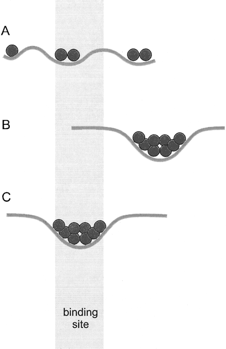
The concept of detecting the funnel by smoothing the landscape is illustrated in Figure 1 ▶. The top landscape is the general energy trend, either flat (Fig. 1A ▶) or funnel-like (Fig. 1B ▶). The real landscape, however, is a rugged surface, with deep local minima and high energy barriers. Thus, the distinction between the flat and the funnel-like real landscapes is obscured by these "high-frequency" fluctuations. The smoothing of the landscape by transition to long-range potentials (∼7 Å for the repulsion part and ∼7 Å for the attraction part; see Vakser 1996a) removes the high-frequency fluctuations and reveals the trend. However, in practice, for the real proteins, such smoothing still leaves low-frequency fluctuations, comparable with the funnel itself.

Fig. 1.

Energy landscapes for intermolecular interactions. Two different landscapes are shown: a flat landscape (A) and a landscape with the funnel at the binding site (B). The real landscape (blue curve) is smoothed by averaging the contribution of neighboring atoms, to reveal the actual form of the landscape. To detect the funnel, one has to separate it from low-frequency energy fluctuations. The red circles are the low-energy ligand positions, determined by a systematic search.

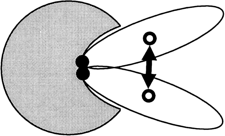
The reason is illustrated in Figure 2 ▶. The extension of the potential range of the "steric" interactions (see Materials and Methods) results in low-resolution molecular shapes (the molecular shape is determined by the repulsion part of the steric interactions). The energy landscape (with our potentials) is determined by the shape of the interacting proteins. Thus, the funnel usually corresponds to the most prominent shape feature (e.g., a deep active site of an enzyme, or a flat multisubunit interface, as in Fig. 2 ▶). By lowering the molecular image resolution, we can reach the point at which only the largest shape characteristic is preserved. This would eliminate all minima but the funnel. Real protein interactions, however, are much more complex than this simple scheme. The interaction is an interplay of shape matches that involves different combinations of structural features of various size. Thus, in reality, the potential range (shape resolution) of ∼7 Å is an empirical compromise between the ability to smooth the landscape and the retaining of funnel-size features.

Fig. 2.

A geometric illustration of the concept of low-resolution protein recognition. The correct position of the ligand within the complex (global minimum of energy) corresponds to a prominently shaped feature. This geometric recognition factor (often the largest one) is still preserved after most of the smaller features are deleted by decreasing the resolution of the molecular image.

The detection of the funnel, from the point of view of protein geometry, is the low-resolution representation of the classical docking problem: how to distinguish between the correct match and the false-positive matches. In our formalism, both geometric and energy landscape interpretations are equivalent. Because the energy landscape concept provides a better understanding of the interaction patterns, in this study we used the energy landscape considerations for the description of protein–protein docking.

Because GRAMM implements the exhaustive search on a grid for low-energy matches, we were able to detect all matches (within the accuracy of the grid) that corresponded to all minima, below a set energy level (Fig. 1 ▶, lower landscapes). Thus, the problem of detecting the funnel becomes a problem of distinguishing between distributions of matches corresponding to the funnel and to the low-frequency landscape fluctuations.

Possible distributions of matches are schematically illustrated in Figure 3 ▶. A random distribution with no major clustering is shown in Figure 3A ▶ (landscape type A). It is characterized by the multiplicity of low-frequency minima—the multiple minima problem at low resolution. Because the size of a low-resolution minimum is substantially larger than the size of a "real" minimum, the number of low-resolution minima is smaller than the number of real minima (the overall size of the landscape is determined by the size of the proteins and is approximately the same at high and at low resolution). However, this number is still significant (potentially, several hundred; the estimate is based on the grid step and the size of proteins). A clustered distribution, with the cluster outside the binding area, is shown in Figure 3B ▶ (landscape type B). At least some of such cases could be attributed to alternative binding modes. The native structure funnel is shown in Figure 3C ▶ (landscape type C).

Fig. 3.

Possible types of the smoothed (low-resolution) energy landscape. The landscape types, identified by the pattern of low-energy ligand positions (red circles) are random (A), clustered outside the known binding site (B), and clustered inside the known binding site (C).

The goal of this study was to determine how many cases of the landscape type C are among the 475 landscapes corresponding to the 475 protein–protein complexes in our database. The difference between types C and B (no minima in the binding area) is quite obvious and easy to detect. The main problem is the difference between types C and A. In reality, we cannot expect that the funnel will be the only low-frequency minimum in a given landscape. Thus, we have to determine whether the minimum found in the binding area is the funnel or just a low-frequency fluctuation. We assume that the fluctuation has to be random. Thus, determining whether the minimum is the funnel is equivalent to determining whether this minimum is significantly different from a would-be random one. The core of the problem is: what is a random minimum? In other words, if we obtain a rational random distribution of minima, we can answer the question posed in the title of this paper: how common is the funnel-like energy landscape in protein–protein interactions? Although, in the beginning, the issue of randomness may look simple, in fact it is very complex and uncertain. In our earlier report (Vakser et al. 1999), we used a simple random model—a homogeneous distribution on a sphere. This model has serious shortcomings, which are described below. In this study, we suggest a set of models, including more sophisticated ones that are based on more realistic representations. The random models are arranged by their complexity. More realistic and complex models have more restrictions on the distribution of matches.

Random models

Definitions

For convenience, the larger and the smaller proteins within a complex are called receptor and ligand, respectively.

A distribution of the ligand's center of mass (CM) within 10 Å from the experimentally determined position is called the binding site. A distribution of the contact residues CM on the receptor within 6 Å from the experimentally determined position is called the contact site. For ideal spherical molecules, the 10 Å and 6 Å values would give approximately equal probabilities to hit either binding or contact site, respectively. Later in the text we also introduce a cutoff-free criterion.

The contact residues on the receptor are at < 7 Å C^β − C^β (C^α for Gly) distance from any of the ligand's residues. We further selected only residues that belong to the receptor's surface. The surface residue was defined as a residue with the side-chain accessible surface >7% of the total (Mizuguchi et al. 1998). The accessible surface was calculated by PSA (Sali and Blundell 1993). This step was necessary because of large interpenetration of molecules in low-resolution predictions (Vakser 1995).

The random distributions are the following: the random distributions of matches (RM) and the random distributions of binding or contact sites (RS).

The probability p_k to obtain k or more hits out of n randomly generated matches (P value) is given by binomial distribution (or by Poisson distribution for large n). Thus, a distribution of matches at the binding/contact site was considered nonrandom (detected funnel) if p_k was <5%.

Model 1. Uniform RM distribution of ligand CM in a box

In model 1, a naÏve model, matches (positions of the ligand's CM) are distributed uniformly in a box around the receptor (Fig. 4 ▶). Because even a trivial docking procedure would exclude predictions in which a ligand is not in contact with the receptor, or placed inside the receptor, such a model must be considered too indiscriminate and unrealistic. Thus, we did not use it in the analysis.

Fig. 4.

Random model 1. Matches (ligand CM, shown by small filled circles) are distributed uniformly in a box around the receptor. This and all other 3D models are shown by 2D cross sections.

Model 2. Uniform RM distribution of ligand CM on a sphere

Model 2 was used in our previous report (Vakser et al. 1999). The model is based on two assumptions: first, the proteins may be roughly considered as spheres, and second, the random matches are uniformly distributed around the receptor (Fig. 5 ▶). Assuming that the atoms are homogeneously distributed in the spheres, we set the radii of the spheres to be such that the average distance of the atoms from the sphere's CM is the same as it is in the real protein. These radii were calculated and taken into account individually for each complex. The funnel detection condition was satisfied for 52% of 475 complexes in the database.

Fig. 5.

Random model 2. Proteins are approximated by spheres. Matches, represented by ligand CM, are placed around the receptor by using the uniform random distribution for each match. The binding site is shown in gray.

The weaknesses of this model are as follows:

1. Both receptor and ligand are described as spherical bodies, and as a result, the random matches are generated on a spherical surface. A more realistic representation of protein surfaces would be more adequate.

2. The uniform distribution of individual matches, used in a random model, leads to the binomial distribution for a set of n matches. For a fixed ratio k/n, the distribution shows strong decrease of P values for larger n (Fig. 6 ▶). A typical distribution of docking results is essentially non-uniform, as discussed below. This prevents the comparison of results obtained by using different subsets of initial 1000 matches. Smaller subsets are put into unfavorable position.

3. A typical distribution of matches is essentially non-uniform (Fig. 7 ▶). The uniform distribution favors the presence of large clusters themselves, with no regard to their position relative to the binding site. To illustrate this, let us consider an artificial procedure of placing matches for nearly spherical molecules, with no regard to their actual complementarity preferences. Let the radius of each molecule be 20 Å. For the parameters described above (1000 matches and 10-Å radius of the binding site), the binomial distribution requires 23 or more hits for the P value <5%. Using the data of Hardin and co-workers (http://www.research.att.com/∼njas/coverings), it is possible to place 82 points on the surface of a 40-Å sphere so that the distance from any point on the sphere to the closest point from these 82 points is <10 Å. On the other hand, if we start putting exactly 23 matches into each point of a given set, we will fill 43 points. If we select 43 points among 82 points to maximize the total area covered by the corresponding 10-Å caps, obviously this area will occupy >50% of the area on the sphere. Thus, on average, wherever the true binding site occurs on a sphere, it is guaranteed that in at least 50% of such dockings, our procedure will generate 23 hits in the binding site; as a result, the P value is <5%. Bringing forward that example, we must stress that our actual docking procedure clusters matches as a result of true surface-to-surface complementarity between the receptor and the ligand. Because of that, the use of a uniform distribution on a sphere as a random model is justified, because it favors cases that exhibit strong positional preferences of the ligand relative to the receptor.

Fig. 6.

The probability to obtain k or more matches in the binding site out of n randomly generated matches (k/n is assumed constant). See text for details.

Fig. 7.

Example of the distribution of matches around the receptor. The receptor is 1wtl, subunit B, and the ligand is 1wtl, subunit A. The CM of the ligand is shown as a black dot, for 1000 lowest-energy positions of the ligand. The open circle (indicated by an arrow) is the actual position of the ligand's CM within the complex. The distribution of the matches reflects clustering on an ∼7-Å grid. Multiple ligand positions in the same grid node occur due to the multiplicity of ligand angular orientations at low resolution (Vakser 1995). For better visualization, matches in the same grid node were randomly shifted by a small interval.

Model 3. Uniform RM distribution of contact CM on a sphere

The predicted ligand CM positions can have large differences in essentially similar configurations of a complex (Fig. 8 ▶). The contact CM positions may better reflect the similarity or dissimilarity of docking modes. Model 3 is equivalent to model 2 with the contact CM positions substituted for ligand CM positions. In this model, the random matches are distributed on a sphere with the radius equal to the estimated radius of the receptor (Fig. 9 ▶).

Fig. 8.

Contact site versus binding site. The receptor is shown in gray. Ligand CM and contact residues CM are shown as open and filled circles, respectively. For many ligands, matches with the similar binding modes may show large differences in the position of the ligand CM.

Fig. 9.

Random model 3. Proteins are approximated by spheres. Matches, represented by contact residues' CM, are placed around the receptor by using the uniform random distribution for each match. The contact site is shown in gray.

Model 4. RM distribution of contact CM on the actual molecule

Model 4 takes into consideration the actual shape of the molecules. For the contact site, we randomly chose the surface residue on the receptor and assigned there the contact site (Fig. 10 ▶). Because, in this case, there is no analytical formula for the distribution of such random matches, we have to calculate corresponding probabilities numerically, by generating a large-enough number of sets. Unfortunately, as we showed above, the RM models introduce undesirable dependency on the number of matches considered for each complex. Thus, we chose to limit our study to simple RM models (models 2 and 3).

Fig. 10.

Random model 4. Matches (contact residues' CM) are randomly distributed on the actual receptor molecule.

Model 5. RS distribution of contact CM on the actual molecule

The RS model is based on the actual distribution of contact CM and the random distribution of the contact site (Fig. 11 ▶). The idea is to check whether a different position of the contact site would contain a large number of hits. In the RS model, the funnel is considered to be detected if the probability of larger or equal number of hits in the random site is <5%. The RS model is free of the RM models shortcoming—dependency on the number of matches considered for each complex. Also, that model will not detect the funnel in the example of the artificial distribution of matches described for model 2.

Fig. 11.

Random model 5. Matches (contact residues' CM) are distributed on the receptor molecule, according to the actual docking results. The position of the contact site (shown in gray) is selected randomly.

Models with clustering

The next set of random models could take into account the clustering of matches, but we did not pursue this approach because the development of increasingly realistic models would reduce their random nature. Instead, they would evolve into a docking procedure, and thus, they would fail the purpose of being naÏve models used for comparison. In the context of the present work, there cannot be the ideal random model. Thus, we restricted this study to already large set of models that are described above.

Models 6 and 7. RM or RS distribution of contact residues

Another statistical distribution is based on the predicted set of contact residues on the receptor. The correctly predicted contact residues in a match were the intersection of the contact residue set in the cocrystallized complex and the contact residues in the match. We calculated the ratio of the number of correctly predicted contact residues n to the total number of predicted contact residues n_m. As we did with the models based on the contact sites, we applied the RM (model 6) and RS (model 7) distributions (Fig. 12 ▶). However, because now a match is a set of residues, rather than one point, as in binding/contact sites models, the statistical analysis is more complex.

Fig. 12.

Random models 6 and 7. The proteins are approximated by spheres (model 6; top) and by actual structures (model 7; bottom). The randomly selected contact residues are shown as bold black curves. The actual contact residues are in gray. See text for details.

Results and Discussion

The database of 475 nonredundant cocrystallized protein–protein complexes was used to re-dock the proteins using smoothed potentials. According to our methodology, the molecules were represented by 3D grid images. In this study, the grid step was 6.8 Å, and thus, all atom-size details were eliminated. The docking procedure provided the list of all low-energy matches, within the precision of the grid (see Materials and Methods for the details). The protein–protein interaction energy landscape was described as the distribution of these matches. Five random models (models 2, 3, 5, 6, and 7) were used to detect the funnel in the landscape. In models 2, 3, and 5, the funnel was considered detected if the statistical criterion (described in definitions under "Random models") was satisfied. The statistical criterion for models 6 and 7 is described later in the text. The results for all tested models are described in detail below.

Funnel detection based on models with 1000 matches

Model 3 yielded the highest percentage of detected funnels, or 59% (results obtained using models 2, 3, and 5 are in Fig. 13 ▶). This number is larger than the one in model 2 (which was 52%; model 2 was used in our earlier study [Vakser et al. 1999]) and in model 5 (33%). However, as we indicated above, this number depends on the size of the contact site cutoff. If the radius for the contact site was the same as the one for the binding site, the difference would be larger.

Fig. 13.

Percentage of detected funnels, obtained by using different random models.

Clustering of matches effect

As discussed earlier, the real distribution of matches is usually clustered, and thus, it is significantly different from the uniform distribution. When the real distribution is compared with the random model (uniform distribution), it is important to know whether the difference can be attributed to the higher density of matches in the binding/contact site area (binding funnel) or to the clustering of matches only (funnel-like landscape in other areas of contact; possibly alternative binding modes). The question is: how many funnels would be detected if the results were based on the random matches models but the actual position of the contact site was unrelated to the real one? In other words, what results would these models yield if the docking was random, in terms of the position of the true contact site, but still had the same pattern as the real docking? To answer this question, we applied the model of random matches (model 3) to the sites generated by the model of random sites (model 5). The funnels were detected in 18% of complexes. Thus, one can assume that out of a 59% detection rate for the prediction of contact site, 18% are the result of the clustering of matches. The origin of this clustering could be alternative binding modes. In part, this assumption was confirmed in a number of cases (Vakser et al. 1999). However, at this point, we cannot generalize this conclusion.

Funnel detection based on models with one match

Another way of funnel detection is to use a single, lowest energy match per complex (Fig. 13 ▶). In this case, the funnel is considered detected if the match appears in the binding/contact site. Because the probability of having such a hit randomly is, on average, ∼1.5%, for both the contact site and the binding site, this assumption is reasonable. As expected, for one match, the model of random contact site (model 5) yields about the same result as the models of random matches (models 2 and 3). Because the models of random matches approximate the surface of the receptor by a sphere, and the model of random contact site—by a set of surface residues (the actual shape of the molecule), the closeness of the results shows that the spherical approximation is quite adequate in our context. A single-match case also provides a better way to check for nonrandom behavior of docking, because we do not have to make any assumptions about the distribution of matches for a particular complex. Specifically, we can reasonably assume in a naÏve model that for each of the 475 complexes, the match is positioned on a corresponding sphere randomly. This assumption is by far less strong than is the previous one about the uniform random distribution of a set of matches. Then the probability to obtain the observed 15% success rate by chance is again given by binomial distribution (the probability of a single success is 1.5%). This probability is zero, within the machine precision limit.

Difference between funnel detection based on 1 and on 1000 matches

The difference in results between 1 match and 1000 matches for the models of random matches (e.g., 15% and 52% for model 2) may be attributed to the clustering of the matches. However, we observed a similar, although less pronounced, difference for the model of random contact sites (15% and 35%, correspondingly). The analysis of this random model showed that there still can be an artificial difference between many matches versus just one match, caused by the definition of the hit. Figure 14 ▶ demonstrates a possible example. If our cutoff distance for the contact site is 6 Å, the two matches are 12 Å apart, and the true contact site is between them (Fig. 14A ▶); then there are two hits in this site. Under these circumstances, the number of possible random contact sites with the same or greater number of matches is zero. On the other hand, let's assume that there is one and only match in the true contact site, exactly in the center of the site (Fig. 14B ▶). Then any random contact site with its center within the 6-Å distance from the match will contain the same one hit (dashed circle in the figure). This means that in our model, despite the obviously better quality of docking in Figure 14B ▶ (direct hit), the probability to obtain the same or greater number of hits randomly is far greater in Figure 14 ▶ B than in A. The use of a cutoff distance in the definition of a hit creates the difference between the cases of many matches and one match. However, a priori, it is difficult to make any judgment about the significance of that feature.

Fig. 14.

Problem with the rigid cutoff definition of the binding/contact site. A more accurate set of matches (A) and a less accurate set of matches (B) are shown. The sites are big circles, the actual position of the ligand's or contact residues' CM are small open circles, and the matches (CM positions) are small filled circles. See text for details.

Funnel detection with modified binding/contact site criterion

To compensate for the cutoff effect, we repeated the calculations with a modified criterion. For each match, we calculated exp(−r/r_c), where r is the distance from the match to the center of the contact site, and r_c is the cutoff distance from the previous criterion. The sum of that expression over all considered matches was used in the model of random contact sites, in the same way that the number of hits was used before. This representation solved the problem described in the previous section. At the same time, it ignored the input from far away matches, similar to the cutoff method. As expected, for 1000 matches, the new criterion yielded results close to the ones obtained using the old (cutoff) criterion (Fig. 15 ▶). However, in case of the single match, the results moved much closer to those of 1000 matches.

Fig. 15.

Percentage of detected funnels, obtained by using model 5 with the smooth cutoff definition of the contact site.

Funnel detection on the basis of clusterization of matches

The new criterion removed the last obstacle for the comparison of funnel detection results by using different subsets of matches. We took advantage of this by exploring a possibility to use clusters of matches instead of individual matches for the funnel detection. In this approach, each cluster is represented by a single match. We grouped matches according to the position of the ligand's CM and sorted these clusters by size (the number of matches in the cluster), by the lowest energy of matches in the cluster, and by the average energy of matches in the cluster. Then we calculated our usual statistics for subsets of matches taken from 1, 10, and 100 first clusters (sorting as described above). From each selected cluster, we took one match with the lowest energy. We also computed the local density of matches for each match and selected matches with the highest density. The local density definition was as follows: for each predicted position of contact site j, we calculate

where d_ij is the distance from i to j predicted contact sites, d_c is the characteristic distance, which was set to 12 Å. This procedure allowed us to pick the prediction that is located in the middle of the largest cluster of other predictions. Such representative matches were determined in the set of all 1000 matches and in the set of lowest energy matches selected in each grid node (in a single grid node, there could be matches that differ in orientation of the ligand but not in the ligand CM position). The number of detected funnels was 29% and 28%, correspondingly, using the random contact sites model with exponential weights (see the description above). This result practically did not differ from the results with simply all 1000 matches or 1 match with the best score. For all the other subsets, the number of detected funnels did not change significantly.

Funnel detection by random matches using contact residues

In the RM-based model, the "true" and the predicted contact surface residues patches are caps on a sphere (see Fig. 18 ▶ in Materials and Methods). The surface area of each cap, divided by the surface area of the sphere, is equal to the number of contact residues on the corresponding surface patch (n_c for the true resides and n_m for the predicted ones) divided by the total number of surface residues on the receptor n_s. The area of the intersection of the caps divided by the whole sphere area is equal to the number of correctly predicted contact residues divided by the total number of surface residues. In our random model, we assumed that the center of the cap corresponding to the prediction might be located at any point on the sphere with equal probability (uniform distribution). If we need to find a probability of having n or more correctly predicted contact residues (P value), we determine the corresponding area of the caps' intersection and the distance d (in spherical geometry) between the caps' centers. Then, any match cap located within that distance from the true site cap will have greater or equal number of correctly predicted contact residues. In our uniform probability distribution, P value becomes equal to the area of the cap with radius d divided by the sphere area (we assume that the sphere has a unit radius). To find d, we need the expression for the area of intersection of two spherical caps. We had to construct it (see Materials and Methods), because it was not readily available in the reference literature.

Fig. 18.

Area of overlap of two spherical caps.

The threshold for n/n_m was defined as 33%. If the ratio was larger than that (i.e., if more than one-third of predicted contact residues are predicted correctly), the match was considered a hit (successful prediction). Using expressions described in Materials and Methods, we determined the probability of a hit in our random model. Then we applied binomial distribution to find the probability of having the same or greater number of hits (P value) than the one observed in the docking results for a given set of matches. As in models 2, 3, and 5, the funnel was considered detected if the P value was <5%. Results are shown in Figure 16 ▶. This model, however, does not work for small sets of matches, because the average probability to get a hit randomly is ∼0.2 (a P value >0.05).

Fig. 16.

Percentage of detected funnels, obtained by using models 6 and 7, and the ratio of the number of correctly predicted contact residues to the total number of predicted contact residues.

Funnel detection by random sites using contact residues

To obtain a random model that is independent of the number of matches, we used the distribution of random contact sites, similar to the CM-based models described earlier. Because this time a site had to be represented by a set of surface residues, we needed to be able to select randomly placed patches of residues on the surface of a molecule. For that purpose, we first projected the receptor molecule onto a 3D grid with a step that is more than two times larger than the van der Waals radius of an atom. In this projection, values of 1 were placed inside and zero values were placed outside the molecule. The surface grid cells were defined as those that have at least one zero-value neighbor. Then we built a list of connected surface cells for each surface cell. On that surface mesh we selected the cell corresponding to one surface residue, then we selected all surface cells connected to this cell, then all surface cell connected to any of the surface cells already selected, and so on. This process continued until the patch covered the required number of surface residues (we tried to build a patch with the same number of residues as in the true contact site). The procedure was repeated starting from other surface residues, to build patches around them. The method tended to build well-packed patches, centered around the selected residues and, thus, was found superior to more simple methods based on traditional residue contact criteria (e.g., C^β − C^β, or atom–atom distances, etc.).

For the true contact patch and for each of the generated patches, we calculated

where N is the number of matches, n_i,max is the maximum possible number of residues that can be predicted correctly in match i, n_i is the number of correctly predicted residues in match i. We discussed earlier the reason why this smooth exponential weighting is better than a rigid cutoff. "Correctly predicted" here means the predicted residues that also belong to the true or to the generated contact site. We calculated the number of generated patches that have the value of the above expression larger or equal to the one computed for the true set of contact residues. That gave us the probability that the distribution of contact sets obtained from docking is randomly related to the true contact set. If that probability was <5%, we considered the funnel in the given complex detected. The results are presented in Figure 16 ▶.

Funnels are easier to detect for larger interfaces

The existence of the funnel in protein–protein interactions' energy landscape is based on the geometric complementarity of the proteins (see the discussion in "Energy landscapes in docking"). Thus, it is natural to expect that larger geometric recognition factors (larger protein–protein interfaces), on average, correspond to more easily detectable funnels. Results shown in Figure 17 ▶ confirm this assumption. In all tested random models, the larger interfaces consistently showed a larger percentage of detected funnels.

Fig. 17.

Percentage of detected funnels and the correct/total number of predicted residues for large interfaces and for all interfaces.

Summary of the results

Funnels in the intermolecular energy landscape were detected in a database of 475 protein–protein complexes by comparing distributions of matches predicted by docking and by random models. A number of random models were developed and used for the funnel detection. The percentage of complexes with the detected funnel (Figs. 13, 15–17 ▶ ▶ ▶ ▶) ranges from 15%–29% (model 5 with 1 match, different definitions of the contact site cutoff) to 60% (79 for larger interfaces; model 3 with 1000 matches).

Conclusions

The goal of this study was to verify the concept of the funnel-like intermolecular energy landscape for protein–protein interactions by use of a series of computational experiments. Our preliminary analysis (Vakser et al. 1999) revealed the existence of the funnel in many protein–protein interactions. However, because of the uncertainties in the modeling of these interactions and the ambiguity of the analysis procedures, the detection of the funnels requires detailed quantitative approaches to the energy landscape analysis. A number of such approaches are presented in this study.

Because of the multiplicity of the local minima, in "real" intermolecular energy, the distinction between the flat and the funnel-like landscapes is obscured by the high-frequency fluctuations (energy minima). Our docking procedure GRAMM smoothes the energy potential and, thus, eliminates most of the local minima. However, in practice, the smoothing still leaves the low-frequency fluctuations, comparable with the funnel itself. Because GRAMM implements the exhaustive search on a grid, we were able to detect all matches (within the precision of the grid), that correspond to all minima, below a set energy level. Thus, the funnel detection problem became a problem of distinguishing between distributions of matches in the funnel and in the low-frequency landscape fluctuations. If we assume that the fluctuations are random, the decision about whether the minimum is the funnel is equivalent to determining whether this minimum is significantly different from a would-be random one.

The core of this problem is the modeling of random matches (random minima). A rational distribution of random matches in a protein–protein complex allows one to determine whether the funnel exists in this complex. The issue of randomness of the protein–protein matches is not simple. The modeling of random matches is based on a number of assumptions and requires elaborate computational procedures for their generation and analysis.

We used the database of 475 nonredundant cocrystallized protein–protein complexes to re-dock the proteins with smoothed potentials. In an extension of our preliminary report (Vakser et al. 1999), we developed a set of sophisticated random models. We presented a detailed analysis of the application of these models to the funnel detection. The number of funnels detected by using different models varies significantly. However, the results confirmed that the funnel may be the general feature in protein–protein association.

The success in detecting the funnel depends on two factors: (1) the docking procedure, which re-creates the intermolecular energy landscape, and (2) the analysis of the energy landscape. In this study, we concentrated on the second aspect of the problem. However, assuming that the funnel is the general feature in protein–protein interactions, to increase the percentage of detected funnels, one needs to increase further the quality of the docking procedures. We plan to address this issue in our future studies.

Materials and methods

Database

The database of protein–protein complexes includes 475 complexes from the Protein Data Bank (Berman et al. 2000). A structure was considered to be a protein–protein complex if it consisted of two or more chains of 30 or more residues. For convenience, the larger and the smaller proteins within a complex were called receptor and ligand, respectively. The database is nonredundant in that no complex has both the receptor and the ligand homologous to the receptor and the ligand of any other complex in the database. The criterion for the homology was >30% sequence identity. The complexes in the database have a >1000-Ų interface area. To minimize the number of crystallization artifacts, we did not consider the protein pairs with smaller interfaces (Janin and Rodier 1995; Tsai et al. 1996; Carugo and Argos 1997).

Docking

The GRAMM docking approach (Katchalski-Katzir et al. 1992; Vakser and Aflalo 1994; Vakser 1995) involves (i) a projection of the two molecules on a 3D grid; (ii) the calculation, using the Discrete Fast Fourier transformation, of a correlation function that assesses the degree of surface overlap and the penetration upon relative shifts of the molecules in three dimensions; and (iii) a scan of the relative orientations of the molecules in 3D. The algorithm provides a list of correlation values that indicate the extent of geometric match between the molecules; each of these values is associated with six numbers describing the relative position (translation and rotation) of the molecules. Thus, the procedure implements an exhaustive grid search for the ligand–receptor structure matches. The overlap of the molecular images is equivalent to the intermolecular energy E calculated with a step-function potential (Vakser 1996a)

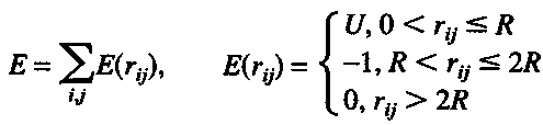where E is the energy, U is the height of the repulsion part of the potential, R is the range of the potential (the grid step), and r_ij is the distance between atoms i (receptor) and j (ligand). The docking parameters in this study were as follows: step of the grid 6.8 Å, repulsion part of the potential 6.5, and interval for rotations 20 degrees. Because the molecules are represented by grid images, no structural details smaller than the step of the grid are taken into account in the calculations. Thus, a sparse grid (in this study, 6.8 Å grid step) eliminates all atom-size details.

Area of overlap of two spherical caps

In spherical geometry, on a sphere with unit radius, the area of a spherical cap is

1

where R is the radius of a spherical circle (solid angle).

The area of a spherical polygon is

2

where N is the number of vertices.

The area of caps intersection is

3

where DAC and DBC are sectors of a circle on a sphere, DC is the intersection of two spherical circles (caps) A and B, and ADBC is the spherical polygon (Fig. 18 ▶).

Using cosine rules for sides (Smart 1960), after some transformations, we obtain the area of intersection

4

where d is the distance (spherical) from A to B (Fig. 18 ▶). We must also take into account the domain of R, r, and d values (where S_DC is constant) when one cap is entirely inside another or the caps do not intersect at all. The expression for S_DC cannot be solved for d analytically. Thus, we solved it numerically, in order to find d as a function of S_DC, which is defined by the number of preserved contact residues n:

Finally, the P-value is (1 − cos(d))/2.

References

- Berg, O.G. and von Hippel, P.H. 1985. Diffusion-controlled macromolecular interactions. Annu. Rev. Biophys. Biophys. Chem. 14 131–160. [DOI] [PubMed] [Google Scholar]
- Berman, H.M., Westbrook, J., Feng, Z., Gilliland, G., Bhat, T.N., Weissig, H., Shindyalov, I.N., and Bourne, P.E. 2000. The Protein Data Bank. Nucleic Acids Res. 28 235–242. [DOI] [PMC free article] [PubMed] [Google Scholar]
- Bridges, A., Gruenke, L., Chang, Y.-T., Vakser, I.A., Loew, G., and Waskell, L. 1998. Identification of the binding site on cytochrome p450 2b4 for cytochrome b5 and cytochrome p450 reductase. J. Biol. Chem. 273 17036–17049. [DOI] [PubMed] [Google Scholar]
- Camacho, C.J., Gatchell, D.W., Kimura, S.R., and Vajda, S. 2000. Scoring docked conformations generated by rigid-body protein–protein docking. Proteins 40 525–537. [DOI] [PubMed] [Google Scholar]
- Carugo, O. and Argos, P. 1997. Protein–protein crystal-packing contacts. Protein Sci. 6 2261–2263. [DOI] [PMC free article] [PubMed] [Google Scholar]
- Chang, Y.-T., Stiffelman, O.B., Vakser, I.A., Loew, G.H., Bridges, A., and Waskell, L. 1997. Construction of a 3D model of cytochrome p450 2b4. Protein Eng. 10 119–129. [DOI] [PubMed] [Google Scholar]
- Dill, K.A. 1999. Polymer principles and protein folding. Protein Sci. 8 1166–1180. [DOI] [PMC free article] [PubMed] [Google Scholar]
- Janin, J. and Rodier, F. 1995. Protein–protein interaction at crystal contacts. Proteins 23 580–587. [DOI] [PubMed] [Google Scholar]
- Katchalski-Katzir, E., Shariv, I., Eisenstein, M., Friesem, A.A., Aflalo, C., and Vakser, I.A. 1992. Molecular surface recognition: Determination of geometric fit between proteins and their ligands by correlation techniques. Proc. Natl. Acad. Sci. 89 2195–2199. [DOI] [PMC free article] [PubMed] [Google Scholar]
- McCammon, J.A. 1998. Theory of biomolecular recognition. Curr. Opin. Struct. Biol. 8 245–249. [DOI] [PubMed] [Google Scholar]
- Mizuguchi, K., Deane, C.M., Blundell, T.L., Johnson, M.S., and Overington, J.P. 1998. JOY: Protein sequence-structure representation and analysis. Bioinformatics 14 617–623. [DOI] [PubMed] [Google Scholar]
- Pappu, R.V., Marshall, G.R., and Ponder, J.W. 1999. A potential smoothing algorithm accurately predicts transmembrane helix packing. Nat. Struct. Biol. 6 50–55. [DOI] [PubMed] [Google Scholar]
- Piela, L., Kostrowicki, J., and Scheraga, H.A. 1989. The multiple-minima problem in the conformational analysis of molecules. Deformation of the potential energy hypersurface by the diffusion equation method. J. Phys. Chem. 93 3339–3346. [Google Scholar]
- Sali, A. and Blundell, T.L. 1993. Comparative protein modeling by satisfaction of spatial restraints. J. Mol. Biol. 234 779–815. [DOI] [PubMed] [Google Scholar]
- Shoemaker, B.A., Portman, J.J., and Wolynes, P.G. 2000. Speeding molecular recognition by using the folding funnel: The fly-casting mechanism. Proc. Natl. Acad. Sci. 97 8868–8873. [DOI] [PMC free article] [PubMed] [Google Scholar]
- Smart, W.M. 1960. Text-book on spherical astronomy, 6th ed. Cambridge University Press, Cambridge, UK.
- Tsai, C.-J., Lin, S.L., Wolfson, H.J., and Nussinov, R. 1996. A dataset of protein–protein interfaces generated with a sequence-order-independent comparison technique. J. Mol. Biol. 260 604–620. [DOI] [PubMed] [Google Scholar]
- Tsai, C.-J., Kumar, S., Ma, B., and Nussinov, R. 1999. Folding funnels, binding funnels, and protein function. Protein Sci. 8 1181–1190. [DOI] [PMC free article] [PubMed] [Google Scholar]
- Vakser, I.A. 1995. Protein docking for low-resolution structures. Protein Eng. 8 371–377. [DOI] [PubMed] [Google Scholar]
- ———. 1996a. Long-distance potentials: An approach to the multiple-minima problem in ligand-receptor interaction. Protein Eng. 9 37–41. [DOI] [PubMed] [Google Scholar]
- ———. 1996b. Low-resolution docking: Prediction of complexes for underdetermined structures. Biopolymers 39 455–464. [DOI] [PubMed] [Google Scholar]
- ———. 1996c. Main-chain complementarity in protein–protein recognition. Protein Eng. 9 741–744. [DOI] [PubMed] [Google Scholar]
- ———. 1997. Evaluation of GRAMM low-resolution docking methodology on the hemagglutinin-antibody complex. Proteins (Suppl. 1) 226–230. [PubMed]
- Vakser, I.A. and Aflalo, C. 1994. Hydrophobic docking: A proposed enhancement to molecular recognition techniques. Proteins 20 320–329. [DOI] [PubMed] [Google Scholar]
- Vakser, I.A., Matar, O.G., and Lam, C.F. 1999. A systematic study of low-resolution recognition in protein–protein complexes. Proc. Natl. Acad. Sci. 96 8477–8482. [DOI] [PMC free article] [PubMed] [Google Scholar]
- Wawak, R.J., Wimmer, M.M., and Scheraga, H.A. 1992. Application of the diffusion equation method of global optimization to water clusters. J. Phys. Chem. 96 5138–5145. [Google Scholar]