Robust Score Statistics for QTL Linkage Analysis

Abstract

The traditional variance components approach for quantitative trait locus (QTL) linkage analysis is sensitive to violations of normality and fails for selected sampling schemes. Recently, a number of new methods have been developed for QTL mapping in humans. Most of the new methods are based on score statistics or regression-based statistics and are expected to be relatively robust to non-normality of the trait distribution and also to selected sampling, at least in terms of type I error. Whereas the theoretical development of these statistics is more or less complete, some practical issues concerning their implementation still need to be addressed. Here we study some of these issues such as the choice of denominator variance estimates, weighting of pedigrees, effect of parameter misspecification, effect of non-normality of the trait distribution, and effect of incorporating dominance. We present a comprehensive discussion of the theoretical properties of various denominator variance estimates and of the weighting issue and then perform simulation studies for nuclear families to compare the methods in terms of power and robustness. Based on our analytical and simulation results, we provide general guidelines regarding the choice of appropriate QTL mapping statistics in practical situations.

Introduction

Recently, a number of new methods have been developed for quantitative trait locus (QTL) mapping in humans by means of general pedigrees. Most of these are based on score statistics or regression-based statistics and attempt to achieve the power of the variance component likelihood-based methods^1,2 while retaining the robustness and computational simplicity of the original Haseman Elston regression.³ In principle, these methods should be preferred over the traditional variance components (VC) approach, which is extremely sensitive to the normality assumption (e.g., see Allison et al.⁴). These new methods are theoretically expected to be relatively robust to non-normality of the trait distribution and also to selected sampling. QTL mapping in humans is typically employed for studying disease-related traits and hence selected sampling schemes are common, making score statistics the obvious choice. However, the literature on these statistics has mostly focused on theoretical development with less attention given to practical issues and implementation. In this paper we address several of the most important practical issues in the computation and use of these statistics.

The score test is a computationally faster, locally most powerful, and robust alternative to the likelihood ratio test. In the context of QTL mapping, this test was proposed by a number of authors (e.g., see^5–9). The score test statistic is simply the partial derivative of the VC likelihood with respect to the “linkage parameter” evaluated under the null hypothesis (no linkage) and standardized by its null standard deviation or an estimate thereof. In this article, we refer to the unstandardized score as the “score function” or the “numerator” and to the standardizing factor as the “denominator.” The aforementioned authors used slightly different parameterizations of the VC likelihood to arrive at the same general formula of the score function for an arbitrary pedigree. The score function remains the same under a broad class of ascertainment schemes (namely ascertainment through phenotype only).^9,10 For sibling pairs, the score function reduces to other statistics like the statistic of Sham and Purcell,¹¹ which were derived independently as direct ways to improve the power of the Haseman-Elston method by incorporating trait squared sums. Similarly, for general pedigrees, an apparently novel statistic¹² was derived by a reverse regression approach (regression of IBD on trait information). A number of the statistics, including the VC method, score statistics, and the reverse regression method,¹² were unified into a common GEE-based framework.^13,14 In particular, their calculations¹⁴ imply the exact equivalence of the numerators of the reverse regression statistic¹² and the score statistic. They also considered the issue of non-Gaussian traits and proposed a numerator incorporating higher moments, which was shown to be robust to non-normality. They considered some higher-moment-based statistics in their simulation study, among a number of other statistics including the VC, score statistics, and the reverse regression statistic.¹² Although their simulations indicate the superiority of higher-moment-based methods for population samples (of Gaussian and non-Gaussian traits), it is not clear whether the higher-moment versions should be preferred over the usual score statistic numerator for selected samples, where accurate trait parameter estimates may not be available.

For the score test to be robust to distributional assumptions, an empirical variance estimate should be used in the denominator to standardize it. This is because the use of empirical variances ensures that the statistic follows an asymptotically normal distribution (by the central limit theorem) and hence preserves correct type I error even if the assumed model is wrong. A number of different denominator variants have been proposed (e.g., see^9,12), ranging from partly to fully empirical variance estimates. Some of these are consistent estimators for the null variance of the score statistic, whereas others are consistent for the true variance. Some condition on the trait values whereas others condition on the identity by descent (IBD) information. The choice of an appropriate denominator is an extremely important issue because it directly affects the power of the linkage statistics. There have been some simulation studies (for selected sibling pairs)^15,16 to investigate denominator variants. For population samples of sibships, some simulations have been conducted,¹⁴ in which a few denominator variants were considered, among other issues. Here again, a comprehensive evaluation of the denominators is required—particularly for selected samples—to identify the best combinations of numerator and denominator in terms of power and robustness.

Traditionally, most QTL-mapping methods neglect the effect of dominance. This is partly because of the computational simplicity under an additive assumption and also because including dominance leads to a loss of power unless the dominance effect is large enough. Two-degree-of-freedom (2 d.f.) score statistics to incorporate dominance have been suggested by a number of authors (e.g., see^17,18). The recent simulation study¹⁴ included a 2 d.f. variance component statistic but not the score statistic. The results of that study indicated that the gain in power of the 2 d.f. VC statistic for a model exhibiting strong dominance may be more than the loss of power when the model is additive. Similar results were reported for a 2 d.f. score statistic in a previous study.¹⁸ Appropriately constructed 2 d.f. score statistics would allow for dominance and will retain other attractive properties such as robustness to selected sampling and non-normality. Here we study the performance of 2 d.f. score statistics vis a vis their 1 d.f. counterparts by using simulation across a variety of models.

Like most linkage mapping statistics, score statistics require some nuisance parameters, namely the population trait mean, variance, and correlation between relative pairs. The higher-moment score statistics require two extra nuisance parameters, the skewness and kurtosis of the trait distribution. These parameters, often called the “segregation parameters,” are independent of the “linkage parameters,” but specifying incorrect values for these parameters may affect the power of the linkage statistic adversely. In a selected sampling situation, or when the sample sizes are small, it is difficult to obtain reliable estimates of these parameters. There have been a few studies (e.g., see^10,15,16) on the effect of misspecification of these parameters on the performance of the score statistics. These studies have generally concluded that some statistics are more sensitive than others to parameter misspecification. They also noted that misspecification of parameters (particularly the trait mean) can have a significant effect on the power of the score statistics. Here we conduct simulations to identify statistics robust to parameter misspecification.

An important issue that has not been dealt with in the literature at all is how to combine pedigrees of different types in an overall score statistic for a data set. Pedigrees of different sizes and structures have different powers to detect linkage, and thus it is natural to think about giving different weights to different pedigrees in an overall statistic. Theoretically, score statistics for individual pedigrees should simply be added (not weighted) to get a score statistic for the entire data set. This is because the nonstandardized scores are on the same linear scale in terms of local power. However, in reality, when conducting a genome scan for a QTL, it would be best to get as much power as possible even for nonlocal alternatives (which the likelihood ratio variance component test achieves at the cost of computational complexity and robustness). A weighted linear combination of pedigree scores may achieve improvement in power, for nonlocal alternatives, while preserving close to optimal power for local alternatives. We address this issue with some analytical calculations as well as limited number of simulations.

All of the simulations in this paper focus on nuclear families, but most of the conclusions generalize to extended pedigrees as well (see Discussion).

Material and Methods

Theory

Notation

Let us consider a data set consisting of K types of pedigrees with n_k pedigrees of type k for k = 1, …, K, each having s_k pedigree members. Let y_ki, M_ki, and Π_ki denote, respectively, the vector of phenotypes, the marker data, and the matrix of estimated pairwise IBD sharing proportions, for the i^th family of type k. Let μ_k, ${\sigma }_k^2$, and Σ_k0 denote the population mean vector, variance vector, and dispersion matrix of the phenotype for the pedigrees of type k. Let Φ_k denote the matrix of kinship coefficients for a family of type k. We also assume that each pedigree of type k is selected according to selection criterion G_k defined purely through its phenotypic data.⁹ Throughout this section, we have omitted the subscript i from expressions such as Var(vec(Π_ki)), which do not depend on i, but only on the structure of the pedigree.

Numerators

A number of authors (e.g., see⁹) have shown that the score statistic for the null hypothesis of “no additive effect of the QTL” under the standard variance components model (for selected and unselected samples) is

$$S_{ki}={v\prime }_{ki}vec({\Pi }_{ki}-2{\Phi }_{ki}),$$ (1)

where

$$v_{ki}=vec[{\Sigma }_{k0}^{-1}(y_{ki}-{\mu }_k)(y_{ki}-{\mu }_k)\prime {\Sigma }_{k0}^{-1}-{\Sigma }_{k0}^{-1}]$$

and vec is an operator that vectorizes the super-diagonal elements of a square matrix in a row-wise order. Under the null hypothesis of no additive variance, the scores S_ki have mean zero and variance $E\left[{v\prime }_{k}Var(vec\left({\Pi }_k\right))v_k{|y_k\in G}_k\right].$ This variance can be estimated with the “conditional on trait value” approach⁸ by ${v\prime }_{ki}Var(vec\left({\Pi }_k\right))v_{ki}$. Thus the score test for no additive variance is a one-sided test based on the standardized statistic:

$$T=\frac{\sum _{k=1}^K\sum _{i=1}^{n_k}{v\prime }_{ki}vec({\Pi }_{ki}-2{\Phi }_k)}{\sqrt{\sum _{k=1}^K\sum _{i=1}^{n_k}{v\prime }_{ki}Var(vec\left({\Pi }_k\right))v_{ki}}},$$ (2)

which has a standard normal distribution under the null. The Var(vec(Π_k)) in the denominator can be estimated either empirically or by simulation, or by using partially empirical methods such as the “imputation” method.¹²

This test statistic can also be expressed as a GEE-based score test.¹⁴ As in Equation (7) of Chen et al.,¹⁴

$$T=\frac{\sum _{k=1}^K\sum _{i=1}^{n_k}{D}_{ki}^{a\prime }{G}_{k0}^{-1}{U}_{ki}^0}{\sqrt{\sum _{k=1}^K\sum _{i=1}^{n_k}{U}_{ki}^{0\prime }{G}_{k0}^{-1}\left(\begin{array}{cc}\mathbf{0}& \mathbf{0}\\ \mathbf{0}& Var(Vec\left({\Pi }_k\right))\end{array}\right)G_{k0}^{-1}{U}_{ki}^0}},$$ (3)

where

$$U_{ki}^0=[(y_{ki}-{\mu }_k)\prime \left\{{(y_{ki}-{\mu }_k)}^2-{\sigma }_k^2\right\}\prime vec\{(y_{ki}-{\mu }_k)(y_{ki}-{\mu }_k)\prime -{\sum }_{k0}\}\prime ],$$

$$D_{ki}^a=\left[\begin{array}{ccc}\mathbf{0}\prime & \mathbf{0}\prime & vec({\Pi }_{ki}-2\Phi )\prime \end{array}\right]\prime ,$$

and G_k0 is the null Gaussian working covariance matrix of $U_{ki}^0$.

By comparing equations (2) and (3), we note that v_ki consists of the last $\left(\begin{array}{c}{s}_k\\ 2\end{array}\right)$ elements of $G_{k0}^{-1}{U}_{ki}^0$. Thus, v_ki is a transformed version of the original phenotype vector, by the Gaussian working covariance matrix.

The GEE formulation was used to construct a new GEE-based robust alternative to the score test,¹⁴ which uses a covariance matrix involving higher moments (skewness and kurtosis) of the phenotype. In analogy with v_ki, we define h_ki as the last $\left(\begin{array}{c}{s}_k\\ 2\end{array}\right)$ elements of $M_{k0}^{-1}{U}_{ki}^0$, where M_k0 is the higher-moment working covariance matrix.¹⁴ Then, a higher-moment score test statistic, as in Equation (11) of Chen et al.,¹⁴ may be simply written as

$$T\left(HM\right)=\frac{\sum _{k=1}^K\sum _{i=1}^{n_k}{h}_{ki}\prime vec({\Pi }_{ki}-2{\Phi }_k)}{\sqrt{\sum _{k=1}^K\sum _{i=1}^{n_k}{h}_{ki}\prime Var\left(vec\left({\Pi }_k\right)\right)h_{ki}}}.$$ (4)

We call h_ki the higher-moment transformed phenotype.

Denominators

For both the Gaussian-transformed phenotype v_ki and the higher-moment transformed phenotype h_ki, we can conceive of different test statistic denominators, depending on how the null variance of the numerator is estimated. The score function for the unconditional likelihood of the data is the same as that based on the likelihood conditioned on trait value or that conditioned on the IBD information.⁸ This means that the statistic remains a valid score statistic (for the appropriate likelihood) irrespective of whether a conditional or unconditional variance estimator is used. The unconditional variance of the score function can be decomposed in two ways as shown below. (Note that we have dropped all the family subscripts in the expressions below for clarity.) Conditioning on trait values we get

$$\begin{array}{c}Var\left[v\prime vec\left(\Pi -2\Phi \right)|y\in \mathbf{G}\right]=Va{r}_y\left[E\left\{v\prime vec\left(\Pi -2\Phi \right)|v,y\in \mathbf{G}\right\}\right]+E_y\left[Var\left\{v\prime vec\left(\Pi -2\Phi \right)|v,y\in \mathbf{G}\right\}\right]\\ =Va{r}_y\left[v\prime E\left\{vec\left(\Pi -2\Phi \right)|v,y\in \mathbf{G}\right\}|y\in \mathbf{G}\right]+E_y\left[v\prime Var\left\{vec\left(\Pi -2\Phi \right)|v,y\in \mathbf{G}\right\}v|y\in \mathbf{G}\right]\end{array}$$

Under the null, this reduces to

$$\begin{array}{c}=0+E_y\left[v\prime Va{r}_{\Pi }\left\{vec(\Pi )\right\}v|y\in \mathbf{G}\right]\left(\text{Variance Conditional on Trait}\right)\end{array}$$ (5)

On the other hand, conditioning on the IBD vector gives

$$\begin{array}{c}Var\left[v\prime vec\left(\Pi -2\Phi \right)|y\in \mathbf{G}\right]=Va{r}_{\Pi }\left[E\left\{v\prime vec\left(\Pi -2\Phi \right)|\Pi ,y\in \mathbf{G}\right\}\right]+E_{\Pi }\left[Var\left\{v\prime vec\left(\Pi -2\Phi \right)|\Pi ,y\in \mathbf{G}\right\}\right]\\ =Va{r}_{\Pi }\left[vec\left(\Pi -2\Phi \right)\prime E\left\{v|\Pi ,y\in \mathbf{G}\right\}|y\in \mathbf{G}\right]+E_{\Pi }\left[vec\left(\Pi -2\Phi \right)\prime Var\left\{v|\Pi ,y\in \mathbf{G}\right\}vec\left(\Pi -2\Phi \right)\prime |y\in \mathbf{G}\right]\end{array}$$

and under the null, this reduces to:

$$\begin{array}{c}=Va{r}_{\Pi }\left[vec\left(\Pi -2\Phi \right)\prime E\left\{v|y\in \mathbf{G}\right\}|y\in \mathbf{G}\right]+E_{\Pi }\left[vec\left(\Pi -2\Phi \right)\prime Var\left\{v|y\in \mathbf{G}\right\}vec\left(\Pi -2\Phi \right)|y\in \mathbf{G}\right]\end{array}$$

Further, under no selection this reduces to:

$$\begin{array}{c}=0+E_{\Pi }\left[vec\left(\Pi -2\Phi \right)\prime Var\left\{v\right\}vec\left(\Pi -2\Phi \right)\right]\left(\text{Variance Conditional on IBD}\right).\end{array}$$ (6)

Note that Equation (5) always gives the correct null variance whereas Equation (6) gives an underestimate of the null variance (and hence inflated type I error) under selected sampling. Depending on which variable is conditioned upon, there can be a number of approaches for constructing the denominator. Also in each case, the means and variances appearing in Equations (5) and (6) can be estimated in different ways, leading to different denominator variants as summarized below.

Approach 1: Conditioning on Trait Value. In this approach, the variance of the score function is computed conditional on the trait values as in Equation (5). This makes the statistic robust to selected sampling. The variance of vec(Π_ki) in the denominator can be estimated in a number of different ways, as follows.

Empirical Variance:

1) SCORE.NULL.CT (variance conditional on trait under null). This statistic uses a conditional on the trait approach with an empirical variance of vec(Π_ki) centered at its null expectation:

$${\widehat{\sigma }}_{NULL.CT}^2=\sum _{k=1}^K\sum _{i=1}^{n_k}{v}_{ki}\prime {\widehat{\mathrm{\Sigma }}}_k^{NULL.CT}{v}_{ki},$$

where

$${\widehat{\mathrm{\Sigma }}}_k^{NULL.CT}=\frac{1}{n_k}\sum _{i=1}^{n_k}vec({\Pi }_{ki}-2{\Phi }_k)vec({\Pi }_{ki}-2{\Phi }_k)\prime .$$

2) SCORE.CT (variance conditional on trait). This statistic also uses a conditional on the trait approach with empirical variance of vec(Π_ki) centered at its sample mean. By its construction, SCORE.CT is expected to have higher power than SCORE.NULL.CT, for samples ascertained with multiple probands, i.e., whenever $E({\Pi }_k|G_k)\ne 2{\Phi }_k$ under the alternative:

$${\widehat{\sigma }}_{CT}^2=\sum _{k=1}^K\sum _{i=1}^{n_k}{v}_{ki}\prime {\widehat{\mathrm{\Sigma }}}_k^{CT}{v}_{ki},$$ (7)

where

$${\widehat{\mathrm{\Sigma }}}_k^{CT}=\frac{1}{n_k-1}\sum _{i=1}^{n_k}vec({\Pi }_{ki}-{\overline{\Pi }}_k)vec({\Pi }_{ki}-{\overline{\Pi }}_k)\prime .$$

We also considered a higher-moment version, HM.CT, of this statistic. This statistic uses the higher-moment numerator as in Equation (4) and the following denominator:

$${\widehat{\sigma }}_{HM.CT}^2=\sum _{k=1}^K\sum _{i=1}^{n_k}{h}_{ki}\prime {\widehat{\mathrm{\Sigma }}}_k^{CT}{h}_{ki}.$$

Note that the above definitions of SCORE.CT and HM.CT do not work when there is only one pedigree of a particular type in a data set. In that case, the sample variance of vec(Π_ki) around its sample mean is zero for that pedigree type. To overcome this problem, an empirical variance around the null expectation, i.e., ${\widehat{\mathrm{\Sigma }}}_k^{NULL.CT}$, is used for such pedigree types. Thus SCORE.CT reduces to SCORE.NULL.CT when there is one pedigree of each type in the data set.

Imputed Variance:

3) SCORE.MERLIN (MERLIN-REGRESS type denominator). This statistic uses the imputed variance estimate of the IBD¹² as implemented in MERLIN-REGRESS (i.e., difference of the prior and posterior variances):

$${\widehat{\sigma }}_{MERLIN}^2=\sum _{k=1}^K\sum _{i=1}^{n_k}{v}_{ki}\prime {\widehat{\mathrm{\Sigma }}}_{ki}^{MERLIN}{v}_{ki},$$

where

$${\widehat{\mathrm{\Sigma }}}_{ki}^{MERLIN}=Var\left(vec\left({\tilde{\mathrm{\Pi }}}_k\right)\right)-Var(vec\left({\tilde{\mathrm{\Pi }}}_{ki}\right)|M_{ki}),$$

where ${\tilde{\mathrm{\Pi }}}_{ki}$ denotes the (unobserved) true IBD matrix.

We also included the higher-moment version HM.MERLIN of this statistic discussed as HM-R in Chen et al.¹⁴ This statistic uses the higher moment numerator as in Equation (4) and the following denominator:

$${\widehat{\sigma }}_{HM.MERLIN}^2=\sum _{k=1}^K\sum _{i=1}^{n_k}{h}_{ki}\prime {\widehat{\mathrm{\Sigma }}}_{ki}^{MERLIN}{h}_{ki}.$$

4) SCORE.MERLIN.AV (MERLIN-REGRESS type denominator with an averaged variance). We considered a modified version of the SCORE.MERLIN estimator:

$${\widehat{\sigma }}_{MERLIN.AV}^2=\sum _{k=1}^K\sum _{i=1}^{n_k}{v}_{ki}\prime {\widehat{\mathrm{\Sigma }}}_k^{MERLIN.AV}{v}_{ki},$$

where

$$\begin{array}{c}{\widehat{\mathrm{\Sigma }}}_k^{MERLIN.AV}=Var\left(vec\right({\tilde{\mathrm{\Pi }}}_k))-\frac{1}{n_k}\sum _{i=1}^{n_k}Var\left(vec\right({\tilde{\mathrm{\Pi }}}_{ki})|M_{ki})\\ =\frac{1}{n_k}\sum _{i=1}^{n_k}{\widehat{\mathrm{\Sigma }}}_{ki}^{MERLIN}.\end{array}$$

Both SCORE.MERLIN and SCORE.MERLIN.AV are motivated by the decomposition:

$$\begin{array}{c}Var\left(vec\right({\tilde{\mathrm{\Pi }}}_k))=Var\left[E\left(vec\left({\tilde{\mathrm{\Pi }}}_{ki}\right)|M_{ki}\right)\right]+E\left[Var\left(vec\left({\tilde{\mathrm{\Pi }}}_{ki}\right)|M_{ki}\right)\right]\\ =Var\left[vec\left({\Pi }_k\right)\right]+E\left[Var\left(vec\left({\tilde{\mathrm{\Pi }}}_{ki}\right)|M_{ki}\right)\right].\end{array}$$

Hence, note that the averaged-variance estimate is expected to give a more accurate estimate of Var(vec(Π_k)) in general, but reduces to the usual estimate when there is exactly one pedigree of each type in the sample (i.e., $n_k=1,\forall k=1,\dots ,K$). Also, note that the denominator variance estimates of vec(Π_ki) for both SCORE.MERLIN and SCORE.MERLIN.AV can theoretically turn out to be negative for the individual pedigree types, particularly when there are few pedigrees of that type in the sample. However, except in the case of extremely small sample size, the overall denominator would turn out to be positive.

Approach 2: Unconditional Variance Approach. In this approach, the variance of the score function is computed unconditionally, i.e., without conditioning on trait or IBD information.

1) SCORE.NULL.EV (fully empirical variance of the score function around its null mean [i.e., 0]). It was discussed as “score-R” in Chen et al.:¹⁴

$${\widehat{\sigma }}_{EV.NULL}^2=\sum _{k=1}^K\sum _{i=1}^{n_k}{S}_{ki}^2.$$

2) SCORE.EV (fully empirical variance of the score function around its sample mean). This is expected to have slightly higher power than SCORE.NULL.EV:

$${\widehat{\sigma }}_{EV}^2=\sum _{k=1}^K\left(\frac{n_k}{n_k-1}\right)\sum _{i=1}^{n_k}(S_{ki}-{\overline{S}}_k{)}^2.$$

When there is only one pedigree of a particular type, the empirical variance for that pedigree type is computed around the null mean (0) of the score (i.e., $S_{ki}^2$). Thus, SCORE.EV reduces to SCORE.NULL.EV when there is exactly one pedigree of each type.

Approach 3: Variance Conditional on IBD.

1) SCORE.NAIVE (naive estimator of variance). This statistic uses a naive estimator of variance for the GEE-based score test. It was discussed as “score” in Chen et al.¹⁴ This statistic uses conditioning on IBD as in Equation (6) with theoretical variance of v_k. It is expected to have incorrect type I error for selected samples and also for non-Gaussian traits:

$${\widehat{\sigma }}_{NAIVE}^2=\sum _{k=1}^K\sum _{i=1}^{n_k}{D}_{ki}^a\prime G_{k0}^{-1}{D}_{ki}^a.$$

We also considered the higher-moment version HM.NAÏVE of this statistic discussed as “HM” in Chen et al.¹⁴ It is expected to be slightly more robust in terms of both type I error and power for non-normal traits but would still have incorrect type I error for selected samples. This statistic uses a higher-moment numerator as in Equation (4) and the following denominator:

$${\widehat{\sigma }}_{HM.NAIVE}^2=\sum _{k=1}^K\sum _{i=1}^{n_k}{D}_{ki}^a\prime M_{k0}^{-1}{D}_{ki}^a.$$

2) SCORE.CIBD (variance conditional on IBD). This statistic uses the conditional on IBD approach, with variance of the transformed trait Var(v_i) estimated empirically centered at the sample mean. This variance is expected to be robust to distributional assumptions (more specifically to misspecification of the working covariance matrix for GEE). However, it can still have incorrect type I error for selected samples:

$${\widehat{\sigma }}_{CIBD}^2=\sum _{k=1}^K\sum _{i=1}^{n_k}\left({\Pi }_{ki}-2{\Phi }_k\right)\prime {\widehat{\mathrm{\Sigma }}}_k^{CIBD}\left({\Pi }_{ki}-2{\Phi }_k\right),$$

where

$${\widehat{\mathrm{\Sigma }}}_k^{CIBD}=\frac{1}{n_k-1}\sum _{i=1}^{n_k}(v_{ki}-{\overline{v}}_k)(v_{ki}-{\overline{v}}_k)\prime .$$

Note that as for SCORE.CT, the denominator empirical estimate of Var(v_ki) for a particular pedigree type becomes zero when there is one pedigree of that type. In such cases, the null expectation of v_ki (i.e., 0) is used to center the empirical variance for that pedigree type.

Approach 4: Minimum Variance Estimator

SCORE.MAX (maximum of SCORE.CT and SCORE.EV). We note that all the denominators considered above (except ${\widehat{\sigma }}_{EV}^2$) are consistent estimators of the null variance of the numerator (provided each n_k tends to infinity). ${\widehat{\sigma }}_{EV}^2$ being fully empirical, it estimates the true variance of the numerator. In general, the smaller the denominator of the test statistic (under the alternative), the higher is the power of the statistic. It is difficult to decide a priori whether the null or alternative variance is smaller, because this depends on the genetic model. We propose the statistic SCORE.MAX with a standard numerator as in Equation (3) and the following denominator:

$${\widehat{\sigma }}_{MAX}^2=\min ({\widehat{\sigma }}_{CT}^2,{\widehat{\sigma }}_{EV}^2).$$

This statistic is effectively a simple maximum of SCORE.CT and SCORE.EV whenever the numerator score is positive. In particular, it is equivalent to the simple maximum in terms of both type I error and power.

Note that this statistic is expected to have correct type I error asymptotically, because the null and true variances are equal under the null. At the same time, it should maintain optimal power under all genetic models. However, for small sample sizes, it is expected to have slightly elevated type I error.

Dominance

For sibship data, because of the orthogonality of π (true IBD between a pair of sibs) and 1_{π = 0.5} (indicator that the pair shares one allele IBD), two orthogonal scores may be obtained and combined easily to form a 2 d.f. statistic.^5,17 Following Tang,¹⁷ we define a 2 d.f. score statistic for sibships as follows. Let Z₁ and Z₂ be the Z-scores corresponding to the scores for the additive variance (α) and dominance variance (δ), respectively. Thus,

$$Z_1=\begin{array}{ccc}\frac{\sum _{k=1}^K\sum _{i=1}^{n_k}{v\prime }_{ki}vec({\Pi }_{ki}-2{\Phi }_k)}{\sqrt{\sum _{k=1}^K\sum _{i=1}^{n_k}{v\prime }_{ki}{\widehat{\mathrm{\Sigma }}}_k^{CT}{v}_{ki}}}& \text{and}& Z_2=\frac{\sum _{k=1}^K\sum _{i=1}^{n_k}{v\prime }_{ki}vec({\mathrm{\Delta }}_k-{\Pi }_{ki}^{\left(1\right)})}{\sqrt{\sum _{k=1}^K\sum _{i=1}^{n_k}{v\prime }_{ki}{\widehat{\mathrm{\Sigma }}}_k^{CT\left(1\right)}{v}_{ki}}}\end{array},$$

where ${\Pi }_{ki}^{\left(1\right)}$ and Δ_k are the estimated and expected matrix of pairwise probabilities of sharing 1 allele IBD, for the i^th pedigree of type k.

${\widehat{\mathrm{\Sigma }}}_k^{CT}$ is given by Equation (7) as before and ${\widehat{\mathrm{\Sigma }}}_k^{CT\left(1\right)}$ is given by:

$${\widehat{\mathrm{\Sigma }}}_k^{CT\left(1\right)}=\frac{1}{n_k-1}\sum _{i=1}^{n_k}vec\left({\Pi }_{ki}^{\left(1\right)}-{\overline{\Pi }}_k^{\left(1\right)}\right)vec\left({\Pi }_{ki}^{\left(1\right)}-{\overline{\Pi }}_k^{\left(1\right)}\right)\prime .$$

Combining these two Z-scores, subject to the constraint 0 ≤ δ ≤ α, gives the 2 d.f. statistic SCORE.2DF.CT, defined as

$$\text{SCORE}.2\mathrm{DF}.\mathrm{CT}=\{\begin{array}{ll}{Z}_1^2+Z_2^2\hfill & \text{if}0\le Z_2\le \left(1/\sqrt{2}\right)Z_1\hfill \\ Z_1^2\hfill & \text{if}{Z}_2\le 0\le Z_1\hfill \\ {\left(\sqrt{2/3}{Z}_1+\sqrt{1/3}{Z}_2\right)}^2\hfill & \text{if}-\left(1/\sqrt{2}\right)Z_2\le Z_1\le \sqrt{2}{Z}_2\hfill \\ 0\hfill & \text{otherwise}\hfill \end{array}.$$

The higher-moment version, HM.2DF.CT, of this statistic can be analogously defined with the higher-moment transformed phenotype h_ki in the numerator instead of v_ki. For extended pedigrees, the orthogonal decomposition does not hold, so a two-parameter score statistic would be needed. The information matrix would involve $Cov({\Pi }_k,{\Pi }_k^{\left(1\right)})$, which can be estimated empirically.

Note that SCORE.2DF.CT and HM.2DF.CT can run into similar problems as SCORE.CT and HM.CT when the sample consists of only one pedigree of a type, in which case they are modified similarly.

Weighting of Pedigrees

Real data often include pedigrees of different sizes and structures. In such cases, it may be desirable to give appropriate weights to each pedigree type so as to obtain maximum power. The advantage of the likelihood ratio test statistic (variance components) is that the weighting is automatic, because the likelihood ratio is evaluated at the maximum likelihood alternative. The score statistic, by contrast, is designed to be locally optimal near the null hypothesis, and under the null hypothesis all pedigrees are weighted equally (or equivalently; standardized scores are weighted in proportion to their null standard deviations). Hence, in most of the score statistic literature, equal weighting of pedigree-wise score statistics has been suggested. However, under alternatives away from the null, it is quite possible that more power can be obtained by using a score statistic with unequal weighting of different pedigrees. For purists who might object that a weighted score statistic is no longer a score statistic, we point out that the object we call the “score statistic” is only approximately the true score anyway. Strictly speaking, the score function (1) is derived under a normal model (conditional on IBD). This is not a very realistic model (because the trait should have a mixture distribution when conditioned on IBD), but it is used as a convenient approximation. The same score function can be shown to have some optimality properties under a mixture-normal model^5,17 and is hence generally accepted. Still, however, in most circumstances the assumption of “normal” or “mixture normal” would fail, and therefore the statistic (1) is no longer technically the score function. Similarly, the higher-moment score function is based on a GEE with an arbitrarily chosen working covariance matrix. When the data violate the higher-moment working covariance structure, this statistic is no longer a “GEE-based score statistic.” Lastly, when population trait parameters are misspecified (e.g., for an ascertained sample), the above statistics are no longer score statistics and may no longer be additive.

Weighting of score statistics may be useful even when the distributional assumption holds. Local optimality ensures that the statistic has optimal power to detect weak effects. The variance component (VC) test is optimal for all alternatives (when the assumed model holds). However, it has the disadvantage of being computationally complex and nonrobust. By weighting pedigrees, it may be possible to increase the nonlocal power of the score statistic while retaining most of the local power and robustness properties.

Let ${\sigma }_a^2$ denote the additive variance and let $\alpha ={\sigma }_a^2/2$. Let us consider n₁ pedigrees of type 1 and n₂ pedigrees of type 2. Let μ_0i, μ_αi, ${\sigma }_{0i}^2$, and ${\sigma }_{\alpha i}^2$ be the null ($H_0:{\sigma }_a^2=0$) and alternative ($H_1:{\sigma }_a^2=2\alpha >0$) means and variances of the score function, respectively, for pedigrees of type i = 1,2. Similarly, we define m_αi, $v_{\alpha i}^2$ to be the means and variances of the standardized score statistic (i.e., centered and scaled to have mean 0 and variance 1). Then, provided n₁ and n₂ are large, the asymptotic optimal weight for linearly combining the standardized Z-scores from the two types of pedigrees is given by the following expression:¹⁹

$$\begin{array}{c}w=\frac{m_{\alpha ,2}/v_{\alpha ,2}^2}{m_{\alpha ,1}/v_{\alpha ,1}^2}\\ =\frac{\left({\mu }_{\alpha ,2}-{\mu }_{0,2}\right){\sigma }_{0,2}{\sigma }_{\alpha ,1}^2}{\left({\mu }_{\alpha ,1}-{\mu }_{0,1}\right){\sigma }_{0,1}{\sigma }_{\alpha ,2}^2}.\end{array}$$ (8)

Therefore, the optimal weight for the nonstandardized score functions is given by:

$$\begin{array}{c}{w}^{\prime }=\frac{\left({\mu }_{\alpha ,2}-{\mu }_{0,2}\right){\sigma }_{\alpha ,1}^2}{\left({\mu }_{\alpha ,1}-{\mu }_{0,1}\right){\sigma }_{\alpha ,2}^2}=\frac{{\mu }_{\alpha ,2}{\sigma }_{\alpha ,1}^2}{{\mu }_{\alpha ,1}{\sigma }_{\alpha ,2}^2}\\ =\frac{m_2^2+2\alpha m_2^3+{\alpha }^2{m}_2^4+({\alpha }^2/2)s_2^2}{m_2^2}\frac{m_1^2}{m_1^2+2\alpha m_1^3+{\alpha }^2{m}_1^4+({\alpha }^2/2)s_1^2}\end{array}$$ (9)

where $m^j=E\{trace\left[{\left({\mathrm{\Sigma }}^{-1}{A}_{\pi }\right)}^j\right]\}$ and $s^j=Var\left\{trace\left[{\left({\mathrm{\Sigma }}^{-1}{A}_{\pi }\right)}^j\right]\right\}$ and subscripts 1 and 2 denote pedigrees of type 1 and 2, respectively. The matrices Σ and A_π have been defined in Appendix A. The above expressions for moments of the score function under population sampling have been derived in Appendix A. Note that the above formula converges to w′ = 1 for local alternatives (α close to 0) but not in general.

The two weights w and w′ defined above are termed as the “standardized optimal weight” and the “nonstandardized optimal weight,” respectively, in the rest of this article.

Simulation

We conducted a simulation study to compare the performance of score statistic variants for nuclear sibships. Our simulation scheme is similar to that described in T. Cuenco et al.¹⁵ A single biallelic quantitative trait and a single marker with 8 equifrequent alleles were simulated. The recombination distance between the two loci was taken as θ = 0.5 and θ = 0 for simulations under the null and alternative hypothesis, respectively.

Genetic Models

The genetic models used are similar to those in T. Cuenco et al.¹⁵ with a decreased locus-specific heritability of 0.15. The details of the models are summarized in Tables 1 and 2. For the first five models (1–5), the trait has a mean depending on genotype plus a normally distributed environmental component. The models 1′–5′ and 1′′–5′′ are non-Gaussian models simulated by subjecting the traits simulated under models 1–5 to the transformations x|x| and x³, respectively. Both these sets of models as well as model 3 (rare recessive trait) are expected to depart substantially from the normality assumption.

Table 1.

Genetic Models: Defining Parameters

	Value for Model
Model Parameters	1	2	3	4	5
Type of inheritance	Add	Dom	Rec	Add	Dom
Locus heritability	0.15	0.15	0.15	0.15	0.15
Allele frequency	0.1	0.1	0.1	0.5	0.5
Trait means	−1,0,1	0,1,1	0,0,1	−1,0,1	0,1,1
Environmental SD	1.010	0.934	0.237	1.683	1.031
Environmental correlation	0.25	0.25	0.25	0.25	0.25

Table 2.

Genetic Models: Population Trait Parameters

	Parameters
Models	Mean	SD	Correlation	Skewness	Kurtosis
Normal Models
1	−0.80	1.095	0.288	0.110	0.058
2	0.19	1.013	0.286	0.092	0.011
3	0.01	0.257	0.257	0.572	2.138
4	0.00	1.826	0.288	0.000	−0.023
5	0.75	1.118	0.275	−0.067	−0.015
Non-normal: x|x|
1′	−1.49	6.758	0.244	−1.660	6.419
2′	0.33	3.379	0.247	1.151	9.094
3′	0.01	0.023	0.241	5.821	65.848
4′	0.00	32.531	0.250	−0.069	8.001
5′	1.41	6.894	0.234	1.726	6.257
Non-normal: x3
1″	−3.22	55.940	0.182	−3.783	26.989
2″	0.69	18.719	0.191	3.649	48.395
3″	0.01	0.022	0.222	12.387	207.990
4″	0.06	524.930	0.180	0.051	36.345
5″	3.11	58.087	0.180	3.759	28.926

Note that our genetic models do not incorporate polygenic effects explicitly. For our purposes, polygenes can be considered to be a part of the shared environment within the family and hence their effect is modeled by considering environmental correlation between relatives.

Selection Schemes

We simulated samples under the following ascertainment schemes: POP (population sampling), SINGLE (single proband sampling with one sib in the top 10% of the trait distribution), ED (extreme discordant sampling with one sib in the top 10% and one in the bottom 10%), EC (extreme concordant sampling with two sibs in the top 10%), EDAC3 (3-corner extreme discordant and concordant sampling with every sibship having a discordant pair at a 12% threshold or a “high concordant” pair at a 4% threshold), and MDAC3 (same as EDAC3 with thresholds of 24% and 8% for discordant and concordant pairs, respectively). Thus, we defined a “discordant” (or “concordant”) sibship as one having at least one discordant (or concordant) sib pair. These ascertainment schemes have been discussed before in the context of sibpairs.^15,16 It is possible to define other notions of concordant and discordant sibships, such as by standard deviation of the sibship trait values,¹⁷ but we consider the above definitions to be more realistic, because sibships are often ascertained through an affected sib or an affected sibpair.

Family Sizes

Most of our simulations were done with sibships of size 4 without parental phenotype information. Parental genotype information was used to estimate IBD sharing between siblings. We did limited simulations with sibships of size 2 and 6, but there were no qualitative differences in the results, except for the expected effects of the increased and decreased sample size, respectively. Hence we report only results for sibships of size 4.

Sample Sizes

The objective of our simulation experiments was to compare the statistics to each other, so the absolute value of power was not considered to be relevant. We chose the sample sizes arbitrarily to keep the power within a reasonable range (i.e., not too high or low) to facilitate comparison across statistics. The sample sizes for the normally distributed data were 450 families for POP samples, 100 for SINGLE, 150 for MDAC3, and 50 each for ED, EC, and EDAC3. The corresponding sample sizes for data transformed with x|x| were 750 (POP), 200 (SINGLE), 300 (MDAC3), and 100 (ED, EC, and EDAC3) and those for data transformed with x³ were 1000 (POP), 300 (SINGLE), 500 (MDAC3), and 200 (ED, EC, and EDAC3).

We used 1,000 and 10,000 replicates to estimate the power and type I error, respectively, at a significance level of 0.01. For computing the analytical thresholds, the asymptotic null distributions of the statistics were used. The null distribution of the 1 d.f. statistics is asymptotically N(0,1), which was used to obtain two-sided p values. The null distribution of the 2 d.f. statistics is asymptotically a mixture of ${\chi }_2^2$, ${\chi }_1^2$, and 0 in the ratio ψ₀/2π : 1/2 : (ψ − ψ₀)/2π, where ${\psi }_0={\tan }^{-1}\left(1/\sqrt{2}\right)$ (see¹⁷), which was used to obtain one-sided p values. For all the type I error and power simulations, the trait parameters were set at their known true values (as given in Table 2). The estimated type I errors for the schemes POP and ED have been summarized in Tables 3A and 3B. The type I errors for the other sampling schemes have been summarized in Table S1A (Type I Errors) available online. The estimated powers of some of the above statistics have been summarized in Tables 4A–4F. The powers of all the statistics have been summarized in Table S1B.

Table 3.

Type I Errors

(A) POPULATIONa	Model 1	Model 1′	Model 1″	Model 2	Model 2′	Model 2″	Model 3	Model 3′	Model 3″	Model 4	Model 4′	Model 4″	Model 5	Model 5′	Model 5″
SCORE.NAÏVE	0.011	0.026	0.063	0.010	0.029	0.087	0.033	0.209	0.295	0.011	0.024	0.065	0.012	0.026	0.072
SCORE.CIBD	0.011	0.011	0.011	0.009	0.012	0.013	0.014	0.015	0.015	0.011	0.011	0.012	0.012	0.013	0.012
SCORE.NULL.CT	0.011	0.011	0.011	0.009	0.012	0.013	0.014	0.015	0.015	0.011	0.011	0.012	0.012	0.013	0.012
SCORE.CT	0.011	0.011	0.011	0.009	0.012	0.013	0.014	0.015	0.015	0.011	0.011	0.012	0.012	0.013	0.012
SCORE.NULL.EV	0.007	0.007	0.005	0.005	0.005	0.004	0.006	0.002	0.001	0.006	0.006	0.005	0.008	0.007	0.006
SCORE.EV	0.007	0.007	0.005	0.006	0.005	0.005	0.006	0.002	0.001	0.007	0.007	0.005	0.008	0.008	0.006
SCORE.MERLIN	0.011	0.011	0.011	0.009	0.012	0.012	0.013	0.016	0.013	0.011	0.011	0.011	0.012	0.013	0.012
SCORE.MERLIN.AV	0.011	0.011	0.011	0.009	0.012	0.013	0.014	0.016	0.015	0.011	0.012	0.012	0.012	0.012	0.012
HM.NAÏVE	0.011	0.025	0.061	0.010	0.031	0.073	0.033	0.220	0.299	0.011	0.021	0.055	0.012	0.024	0.066
HM.MERLIN	0.011	0.011	0.010	0.009	0.011	0.010	0.013	0.012	0.013	0.011	0.011	0.011	0.012	0.013	0.012
HM.CT	0.011	0.012	0.010	0.009	0.011	0.010	0.013	0.012	0.014	0.011	0.011	0.011	0.012	0.013	0.011
SCORE.MAX	0.011	0.011	0.012	0.009	0.013	0.015	0.015	0.016	0.015	0.011	0.013	0.014	0.012	0.014	0.014
SCORE.2DF.CT	0.011	0.011	0.011	0.010	0.012	0.012	0.013	0.018	0.015	0.010	0.012	0.011	0.011	0.012	0.012
HM.2DF.CT	0.011	0.012	0.011	0.010	0.011	0.014	0.014	0.017	0.019	0.010	0.012	0.012	0.011	0.012	0.013
(B) EDb
SCORE.NAÏVE	0.178	0.148	0.133	0.174	0.179	0.155	0.225	0.314	0.341	0.168	0.191	0.155	0.164	0.145	0.125
SCORE.CIBD	0.015	0.015	0.015	0.016	0.015	0.012	0.016	0.017	0.015	0.015	0.015	0.013	0.013	0.014	0.013
SCORE.NULL.CT	0.011	0.011	0.011	0.012	0.012	0.011	0.013	0.016	0.014	0.011	0.012	0.011	0.010	0.010	0.010
SCORE.CT	0.012	0.012	0.012	0.013	0.013	0.011	0.014	0.016	0.014	0.012	0.012	0.012	0.011	0.010	0.011
SCORE.NULL.EV	0.005	0.006	0.005	0.005	0.007	0.005	0.002	0.002	0.001	0.005	0.006	0.005	0.004	0.005	0.005
SCORE.EV	0.007	0.007	0.006	0.008	0.009	0.005	0.005	0.002	0.002	0.008	0.008	0.006	0.007	0.007	0.005
SCORE.MERLIN	0.012	0.012	0.012	0.013	0.013	0.010	0.015	0.016	0.016	0.013	0.011	0.012	0.011	0.010	0.010
SCORE.MERLIN.AV	0.012	0.012	0.011	0.012	0.012	0.011	0.014	0.016	0.015	0.013	0.012	0.012	0.011	0.010	0.011
HM.NAÏVE	0.178	0.109	0.065	0.174	0.139	0.085	0.212	0.295	0.312	0.169	0.144	0.092	0.164	0.114	0.060
HM.MERLIN	0.012	0.010	0.011	0.013	0.012	0.011	0.014	0.016	0.012	0.013	0.012	0.010	0.011	0.011	0.011
HM.CT	0.012	0.011	0.012	0.013	0.013	0.011	0.014	0.015	0.012	0.013	0.012	0.010	0.011	0.011	0.011
SCORE.MAX	0.012	0.013	0.014	0.014	0.015	0.013	0.015	0.017	0.016	0.013	0.014	0.014	0.012	0.012	0.012
SCORE.2DF.CT	0.010	0.011	0.011	0.013	0.012	0.010	0.014	0.016	0.015	0.012	0.011	0.009	0.010	0.011	0.011
HM.2DF.CT	0.010	0.011	0.011	0.013	0.013	0.011	0.015	0.018	0.016	0.012	0.012	0.009	0.010	0.011	0.012

Type I error values departing by 0.005 or more, from the nominal value 0.01, are highlighted in bold.

^aType I errors under population sampling.

^bType 1 errors under extreme discordant sampling.

Table 4.

Power Comparisons

(A) POPULATIONa	Model 1	Model 1′	Model 1′′	Model 2	Model 2′	Model 2′′	Model 3	Model 3′	Model 3′′	Model 4	Model 4′	Model 4′′	Model 5	Model 5′	Model 5′′
SCORE.NAÏVEb	0.74			0.73			0.65			0.75			0.74
SCORE.CIBD	0.74	0.39	0.14	0.73	0.78	0.45	0.53	0.96	0.94	0.76	0.69	0.31	0.74	0.44	0.15
SCORE.CT	0.74	0.39	0.14	0.73	0.78	0.45	0.53	0.96	0.94	0.76	0.69	0.31	0.74	0.44	0.15
SCORE.EV	0.67	0.35	0.11	0.68	0.73	0.40	0.24	0.75	0.73	0.70	0.65	0.32	0.70	0.41	0.11
SCORE.MERLIN	0.74	0.39	0.14	0.73	0.78	0.45	0.53	0.97	0.95	0.75	0.68	0.31	0.74	0.44	0.16
HM.NAÏVEb	0.74			0.73			0.62			0.75			0.74
HM.MERLIN	0.74	0.37	0.14	0.73	0.74	0.48	0.51	0.92	0.91	0.75	0.67	0.34	0.75	0.42	0.16
HM.CT	0.74	0.36	0.14	0.73	0.74	0.49	0.51	0.90	0.91	0.76	0.67	0.33	0.74	0.42	0.16
SCORE.MAX	0.74	0.41	0.16	0.74	0.81	0.50	0.53	0.98	0.96	0.76	0.71	0.37	0.75	0.46	0.18
SCORE.2DF.CT	0.71	0.37	0.14	0.72	0.75	0.43	0.62	0.98	0.97	0.72	0.66	0.29	0.76	0.45	0.15
HM.2DF.CT	0.71	0.34	0.12	0.72	0.70	0.45	0.58	0.93	0.91	0.72	0.62	0.32	0.76	0.42	0.16
(B) SINGLEc
SCORE.CT	0.69	0.78	0.54	0.70	0.78	0.53	0.79	0.99	0.99	0.38	0.43	0.24	0.20	0.19	0.12
SCORE.EV	0.59	0.71	0.49	0.59	0.74	0.52	0.40	0.93	0.92	0.29	0.37	0.18	0.13	0.16	0.09
SCORE.MERLIN	0.69	0.78	0.53	0.69	0.78	0.55	0.80	1.00	0.99	0.38	0.43	0.23	0.20	0.19	0.12
HM.MERLIN	0.69	0.81	0.66	0.69	0.73	0.58	0.78	0.99	0.99	0.38	0.38	0.22	0.20	0.17	0.11
HM.CT	0.69	0.80	0.65	0.69	0.73	0.57	0.76	0.98	0.98	0.38	0.37	0.22	0.20	0.17	0.11
SCORE.MAX	0.70	0.81	0.61	0.70	0.80	0.61	0.79	1.00	0.99	0.39	0.45	0.28	0.21	0.20	0.13
SCORE.2DF.CT	0.66	0.76	0.52	0.65	0.75	0.51	0.85	1.00	0.99	0.36	0.40	0.21	0.21	0.20	0.11
HM.2DF.CT	0.66	0.78	0.63	0.65	0.70	0.53	0.83	0.99	0.99	0.36	0.35	0.21	0.22	0.18	0.11
(C) EDd
SCORE.CT	0.59	0.78	0.74	0.59	0.81	0.85	0.15	0.77	0.92	0.25	0.77	0.87	0.53	0.68	0.70
SCORE.EV	0.48	0.70	0.72	0.52	0.78	0.85	0.04	0.43	0.75	0.18	0.73	0.85	0.46	0.64	0.70
SCORE.MERLIN	0.60	0.79	0.74	0.59	0.81	0.85	0.15	0.78	0.93	0.23	0.77	0.87	0.52	0.67	0.69
HM.MERLIN	0.59	0.82	0.84	0.59	0.81	0.90	0.14	0.70	0.89	0.15	0.77	0.91	0.52	0.69	0.77
HM.CT	0.59	0.81	0.85	0.59	0.80	0.90	0.15	0.68	0.87	0.14	0.77	0.91	0.52	0.70	0.76
SCORE.MAX	0.60	0.79	0.79	0.60	0.83	0.89	0.15	0.82	0.95	0.25	0.79	0.89	0.55	0.71	0.76
SCORE.2DF.CT	0.55	0.75	0.71	0.56	0.79	0.85	0.18	0.88	0.97	0.22	0.74	0.84	0.54	0.69	0.71
HM.2DF.CT	0.55	0.79	0.81	0.56	0.77	0.88	0.17	0.77	0.91	0.15	0.73	0.89	0.54	0.70	0.77
(D) ECe
SCORE.CT	0.61	0.75	0.69	0.55	0.68	0.57	0.81	0.99	1.00	0.23	0.26	0.22	0.12	0.10	0.09
SCORE.EV	0.48	0.63	0.61	0.40	0.62	0.55	0.46	0.88	0.98	0.13	0.18	0.18	0.07	0.07	0.07
SCORE.MERLIN	0.60	0.74	0.69	0.53	0.68	0.58	0.81	0.99	1.00	0.22	0.26	0.23	0.11	0.10	0.09
HM.MERLIN	0.60	0.76	0.74	0.53	0.63	0.65	0.81	0.99	1.00	0.22	0.25	0.25	0.12	0.10	0.11
HM.CT	0.60	0.75	0.73	0.53	0.63	0.65	0.79	0.98	1.00	0.22	0.25	0.24	0.11	0.10	0.11
SCORE.MAX	0.62	0.77	0.75	0.55	0.70	0.64	0.81	0.99	1.00	0.23	0.28	0.27	0.13	0.11	0.10
SCORE.2DF.CT	0.57	0.71	0.65	0.51	0.65	0.54	0.86	1.00	1.00	0.19	0.25	0.21	0.12	0.11	0.09
HM.2DF.CT	0.57	0.72	0.69	0.51	0.61	0.61	0.85	0.99	1.00	0.19	0.23	0.23	0.12	0.11	0.12
(E) EDAC3f
SCORE.CT	0.60	0.73	0.66	0.55	0.71	0.64	0.78	0.99	1.00	0.44	0.57	0.45	0.38	0.29	0.18
SCORE.EV	0.49	0.66	0.62	0.46	0.65	0.61	0.48	0.92	0.98	0.35	0.51	0.42	0.30	0.24	0.14
SCORE.MERLIN	0.60	0.73	0.66	0.55	0.71	0.63	0.78	1.00	1.00	0.44	0.56	0.46	0.37	0.29	0.18
HM.MERLIN	0.61	0.77	0.80	0.54	0.66	0.62	0.79	0.99	1.00	0.44	0.50	0.40	0.37	0.22	0.13
HM.CT	0.61	0.76	0.80	0.55	0.66	0.61	0.79	0.99	1.00	0.45	0.50	0.40	0.38	0.22	0.13
SCORE.MAX	0.61	0.74	0.71	0.56	0.74	0.71	0.78	1.00	1.00	0.46	0.59	0.51	0.39	0.32	0.20
SCORE.2DF.CT	0.56	0.70	0.61	0.52	0.68	0.59	0.85	1.00	1.00	0.42	0.51	0.41	0.40	0.29	0.17
HM.2DF.CT	0.56	0.74	0.77	0.52	0.63	0.56	0.84	0.99	1.00	0.42	0.45	0.37	0.40	0.22	0.13
(F) MDAC3g
SCORE.CT	0.74	0.73	0.50	0.69	0.85	0.64	0.59	0.98	0.98	0.63	0.68	0.44	0.56	0.42	0.20
SCORE.EV	0.66	0.69	0.48	0.62	0.81	0.62	0.25	0.86	0.92	0.56	0.64	0.41	0.50	0.38	0.17
SCORE.MERLIN	0.74	0.73	0.50	0.68	0.85	0.65	0.58	0.98	0.99	0.63	0.68	0.44	0.57	0.42	0.19
HM.MERLIN	0.73	0.80	0.67	0.68	0.79	0.64	0.59	0.98	0.98	0.63	0.64	0.44	0.57	0.38	0.17
HM.CT	0.73	0.79	0.65	0.69	0.80	0.63	0.59	0.97	0.97	0.63	0.65	0.44	0.57	0.38	0.17
SCORE.MAX	0.74	0.75	0.56	0.70	0.86	0.72	0.59	0.98	0.99	0.63	0.70	0.50	0.57	0.44	0.22
SCORE.2DF.CT	0.71	0.69	0.48	0.67	0.83	0.61	0.66	0.99	0.99	0.60	0.65	0.41	0.58	0.43	0.19
HM.2DF.CT	0.71	0.75	0.62	0.67	0.76	0.60	0.66	0.97	0.97	0.60	0.60	0.40	0.58	0.38	0.17

For each model, power values within 3% of the maximum are highlighted in bold.

^aPower comparison for population sampling.

^bWe have dropped power values for SCORE.NAIVE and HM.NAIVE in the case of non-normal models, for which they have theoretically incorrect type I error.

^cPower comparison for single proband ascertainment.

^dPower comparison for extreme discordant sampling.

^ePower comparison for extreme concordant sampling.

^fPower comparison for EDAC-3 corner sampling.

^gPower comparison for MDAC-3 corner sampling.

Sensitivity Analysis

To evaluate the robustness of the statistics to misspecification of population trait parameters, we carried out sensitivity analysis by simulation. For these simulations, we chose four selection schemes (POP, ED, EC, and EDAC) and six models (2, 2′, 2′′ and 4, 4′, 4′′). The five trait parameters (namely mean, variance, correlation, skewness, and kurtosis) were in turn set at two arbitrary wrong guesses on either side of the true value, while holding the other four parameters fixed at their true values. The misspecified parameter values have been listed in Table 5. Power was then estimated based on the same 1000 replicates of data, for each combination of parameter values. This process was repeated for all the combinations of models and selection schemes. SCORE.NAÏVE and HM.NAÏVE have theoretically incorrect type I error when parameters are incorrect. SCORE.CIBD has theoretically incorrect type I error for selected samples. So, these three statistics were dropped from this analysis. The results of the sensitivity analysis have been summarized in Figures 1 and 2.

Table 5.

Sensitivity Analysis: Misspecified Parameters

Model	2			2′			2″			4			4′			4″
Parameter	True	Lower	Upper	True	Lower	Upper	True	Lower	Upper	True	Lower	Upper	True	Lower	Upper	True	Lower	Upper
Mean	0.19	−0.80	1.20	0.33	−2.70	3.30	0.69	−3.30	4.70	0.00	−2.00	2.00	0.00	−10.00	10.00	0.06	−40.00	40.00
Variance	1.03	0.03	2.03	3.38	0.40	6.40	18.72	3.70	33.70	3.33	0.33	6.33	32.53	12.53	52.53	524.93	324.93	724.93
Correlation	0.29	0.10	0.50	0.25	0.10	0.40	0.19	0.05	0.35	0.29	0.10	0.50	0.25	0.10	0.40	0.18	0.05	0.35
Skewness	0.09	−0.90	1.10	1.15	−2.80	3.20	3.65	−16.40	23.60	0.00	−1.00	1.00	−0.07	−5.00	5.00	0.05	−25.00	25.00
Kurtosis	0.01	−2.00	2.00	9.09	3.10	15.10	48.40	−11.60	108.40	−0.02	−2.00	2.00	8.00	−2.00	18.00	36.35	−13.70	86.30

Figure 1.

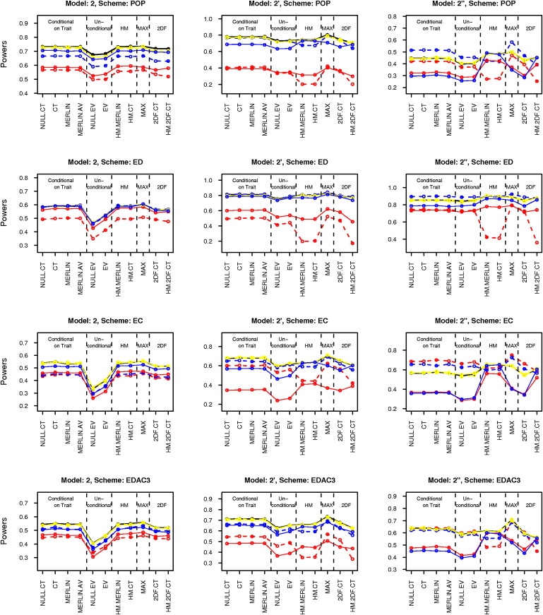
Sensitivity Analysis Results for Mean, Variance, and Correlation

Black line gives power for true parameter values. Solid and dashed lines are for over- and underspecification of parameters, respectively. Line colors red, yellow, and blue stand for misspecified mean, variance, and correlation, respectively. Note that the black line roughly coincides with yellow line in almost all cases.

Figure 2.

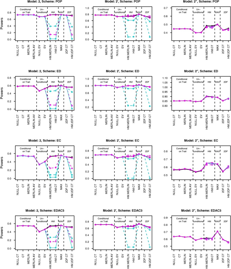
Sensitivity Analysis Results for Skewness and Kurtosis

Black line gives power for true parameter values. Solid and dashed lines are for over- and underspecification of parameters, respectively. Line colors cyan and magenta stand for misspecified skewness and kurtosis, respectively. Note that the black line coincides with the cyan and magenta lines for lower-moment statistics.

Weighting

As described in the previous section, Equation (9) can be used to derive optimal weights for sibships of various sizes for different alternative values of the parameter (under population sampling.) We plotted the optimal weights, as a function of heritability (h²) for sibships of sizes 3, 4, 5, and 6 with respect to sibpairs (Figure 3). For sibships of size 3 versus sibpairs, we also plotted the behavior of the analytical power curve¹⁹ of SCORE.NAÏVE for different values of h² (Figure 4).

Figure 3.

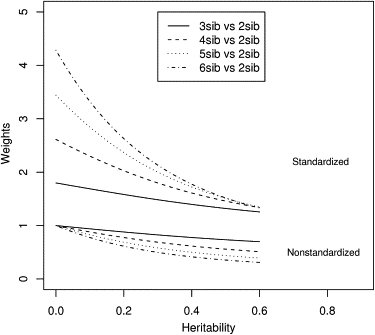
Analytical Optimal Weights for Sibships

Plot of asymptotic optimal weights (analytical) for sibships of sizes 3, 4, 5, and 6 (with respect to a sibship of size 2) as a function of heritability. The lower cluster of plots shows the optimal weights for nonstandardized scores and the upper shows those for standardized scores.

Figure 4.

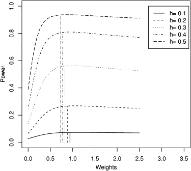
Analytical Power Curves of SCORE.NAÏVE for 3 Sibs

Approximate analytical power curves for a population sample with 100 sibships of size 3 and 100 sibpairs. Power is plotted as a function of nonstandardized weight of 3 sibs with respect to 2 sibs. Curves are shown for five different values of heritability (h²). The vertical lines show asymptotic optimal weights for each value of h².

When we have an ascertained sample (for example, an EDAC sample), Equation (9) no longer holds. But Equation (8) can be used to derive the optimal weight for discordant pairs with respect to concordant pairs, where the means and variances are conditional on the ascertainment scheme and can be obtained by numerical integration. Alternatively, power can also be estimated by using simulation over a grid of different weights. Figure 5 shows the simulation-based power of SCORE.CT for a mixed sample of 20 extreme discordant pairs (one sib in each of higher and lower 10% tails) and 30 extreme concordant pairs (both sibs in the top 10% tail), as a function of the nonstandardized weight of a discordant pair with respect to a concordant pair.

Figure 5.

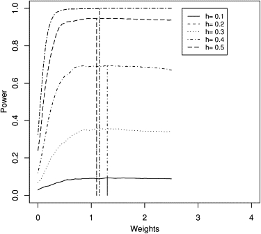
Empirical Power Curves of SCORE.CT for EDAC Pairs

Plot of simulation-based power for a combined sample of 20 discordant pairs and 30 concordant pairs. Power is plotted as a function of nonstandardized weight of discordant with respect to concordant pairs. Curves are shown for five different values of heritability (h²). The vertical lines show the actual optimal weights based on simulation, for each value of h².

Results

Simulation Results

The type I errors for the population and extreme discordant sampling schemes have been tabulated in Tables 3A and 3B and for other sampling schemes in Table S1A (Type I Errors). Most of the statistics have close to correct type I error even for the smallish sample sizes that we used. The type I errors for SCORE.NAIVE and HM.NAÏVE are highly inflated for non-normal as well as selected samples. Similarly, in some cases, the type I error of SCORE.CIBD are inflated for selected samples. Theoretically, all three of these statistics have inflated type I error for selected samples. On the other hand, SCORE.NULL.EV and SCORE.EV have highly conservative type I error. The SCORE.MAX statistic has negligibly inflated type I errors, compared to SCORE.CT. All the statistics except HM.CT and HM.MERLIN have slightly incorrect type I error, in most cases, for the highly skewed models 3′ and 3′′. The higher-moment statistics in general give better type I errors than their lower-moment counterparts, particularly for the non-normal models. In most cases, however, the difference is marginal.

The estimated power for all the models and sampling schemes is summarized in Tables 4A–4F. SCORE.NAÏVE, HM.NAÏVE, and SCORE.CIBD have been dropped from Tables 4A–4F, because they have theoretically incorrect type I error for selected samples. To facilitate comparison, we have also dropped SCORE.NULL.CT, SCORE.NULL.EV, and SCORE.MERLIN.AV from the power tables (Tables 4A–4F). SCORE.CT and SCORE.EV are consistently (and sometimes significantly) more powerful than SCORE.NULL.CT and SCORE.NULL.EV, respectively, while the type I errors are negligibly higher. SCORE.MERLIN.AV has also been dropped, because it fails to provide significant improvement of power over SCORE.MERLIN under most genetic models and selection schemes. In fact, it has slightly reduced power in many cases. The detailed results with all the statistics are given in Table S1B (Power Results).

For all the models and schemes, the unconditional empirical variance denominator SCORE.EV performs poorly. It has low power and a conservative type I error, which can be attributed to the smallish sample sizes. In their simulations, Chen et al.¹⁴ observed similar behavior for SCORE.NULL.EV (denoted as score-R in their paper).

For population samples, under normal models (1, 2, 4, and 5), all the statistics perform essentially identically. SCORE.NAÏVE, HM.NAÏVE, and SCORE.CIBD have similar power to the other statistics. As noted previously,¹⁴ the higher-moment (HM) statistics perform at par with the lower-moment (LM) statistics in this case.

For population samples under non-normal models, SCORE.NAÏVE and HM.NAIVE have inflated type I error. The HM statistics show improvement in power for only some cases, which disagrees with the previous conclusion¹⁴ that HM statistics are always better for non-normal models. Generally, for the x|x| models, which can be thought of as being “relatively less non-normal,” the higher-moments statistics are worse than their lower-moment counterparts. For the “relatively more non-normal” x³ models, there is a marked improvement in the performance of the HM statistics in all the cases.

The relative performance of the statistics follows a similar general pattern for population and selected sampling. The conditional on trait variance SCORE.CT performs as well as SCORE.MERLIN, neither of them being consistently better than the other. The two-degree-of-freedom statistics show some improvement for the dominant model 5 and the recessive model 3 and the transformed versions of these models, but are worse for all the other models. The higher-moment extensions of SCORE.CT, SCORE.MERLIN, and SCORE.2DF.CT usually perform worse for x|x| models (except 1′) and better for the x³ models (except 3′). This is true for all the sampling schemes except EDAC3 and MDAC3, in which the HM statistics are worse for both x|x| and x³ models. The SCORE.MAX statistic is close to optimal in most cases, except for a few cases when the higher-moment statistics or the two-degree-of-freedom statistics have higher power.

Sensitivity Analysis Results

In Figures 1 and 2, we have plotted the sensitivity analysis results for models 2, 2′, and 2′′ and for all four selection schemes, POP, ED, EC, and EDAC. The results for models 4, 4′, and 4′′ were similar. As seen in Figure 1, misspecification of the variance does not affect the power significantly. However, misspecification of the mean or the correlation seems to affect the power of all the statistics considerably. Also as seen in Figure 2, misspecification of the skewness and the kurtosis can reduce the power of the higher-moment statistics drastically in some cases. There was no perceivable difference in sensitivity among the different lower-moment (LM) statistics (or among the HM statistics).

For normal models, power always decreases when parameters are misspecified, because the true parameter values give the optimally powered score statistics. But for non-normal models, in some cases (e.g., underspecification of correlation in model 2′′ for population sampling), power may increase by using wrong parameter values, as the true scores are not necessarily optimal under these models.

For normal models (e.g., model 2), under population sampling, the effects of mean and correlation are symmetric. In other words, overspecification and underspecification have roughly equal effect. However, for non-normal models (e.g., 2′ and 2′′) or under selected sampling, the effects can be asymmetric. The direction of asymmetry can also change across selection schemes. Also, underspecification of mean and correlation seems to be better than overspecification for LM statistics whereas the order reverses for HM statistics.

For normal models (e.g., model 2), the LM and HM statistics are equally sensitive to mean and correlation. However, the HM statistics have the additional dependence on the skewness and kurtosis parameters, to which they are highly sensitive for these models. For slightly non-normal models (e.g., 2′), both the LM and HM statistic are highly sensitive to the mean. The HM (respectively LM) statistics are more sensitive to the mean for the ED (respectively EC) scheme. The HM statistics are highly sensitive to skewness and kurtosis, especially to underspecification of these parameters.

For highly non-normal data (e.g., 2′′), the LM statistics are highly sensitive to mean and correlation, especially to overspecification of these parameters. Underspecification can sometimes provide increase in power. In some cases (e.g., EC and EDAC3), the HM statistics are relatively less affected by mean and correlation. For the ED scheme, the HM statistics are strongly affected by misspecification of mean. However, they are quite stable with respect to skewness and kurtosis for all sampling schemes, under these models.

In summary, misspecification of mean or correlation can have significant effect on the power of both LM and HM statistics. Effects can be asymmetric for skewed models or under selected sampling, and the direction of asymmetry is generally different for LM and HM statistics. Misspecification of skewness and kurtosis can have drastic effect on the power of HM statistics, particularly for normal and slightly non-normal models. However, for highly non-normal models, the HM statistics are stable with respect to skewness and kurtosis and also, in some cases, less sensitive than LM statistics to specification of mean and correlation.

Weighting Results

The results of the weighting experiments are summarized in Figures 3–5. As shown in Figure 3, for population samples, the optimal weights for the larger sibships (with respect to sibpairs) decrease with increase of heritability. The nonstandardized optimal weight also decreases with increasing sibship size. However, as expected, the standardized optimal weights are all greater than 1 and increase with sibship size (larger sibships are more informative and hence the corresponding standardized Z-scores receive higher weight).

Figure 4 shows that the power curves are usually flat to the right of the optimal weight. Because 1 lies on the flatter side of the peak, a nonstandardized weight of 1 does not lead to much loss of power even for large effect sizes.

The power curve in Figure 5 is similar to those of Figure 4, but the peaks cluster closer to 1. Hence even for EDAC samples there is no obvious gain by using unequal weights on the nonstandardized scores for discordant and concordant pairs. Our experiments with mixtures of random pairs and concordant/discordant pairs gave similar results (data not shown).

Discussion

We have conducted a comprehensive simulation study of some of the existing variants of score statistics as well as some novel ones. Our study attempted to identify the most robust score-based statistics under various genetic models and sampling schemes. The proposed conditional on trait variance (SCORE.CT) outperformed the empirical variance denominator (SCORE.EV), which has been suggested by many articles on score statistics. SCORE.EV appears to have a highly conservative type I error for small sizes and hence low power. This fact, also observed previously,¹⁴ is probably due to the fact that the scores (being a quadratic function of the trait values) are considerably skewed and hence it requires large sample sizes for the central limit theorem to apply. Whereas when we condition on the trait, the IBD vector has a symmetric distribution around its expectation (under the null) and hence the central limit theorem is applicable for smaller sample sizes. SCORE.CT also matches the power of SCORE.MERLIN in most cases and sometimes exceeds it. These two statistics differ only in the computation of the variance of the IBD vector in the denominator. SCORE.MERLIN uses the method of imputation¹² and requires the joint distribution of pairwise IBDs for its computation. Limited experiments suggested that computation of SCORE.MERLIN can be slow for large pedigrees with uninformative markers or many ungenotyped individuals (data not shown). On the other hand, SCORE.CT is easier and much faster to compute because it involves a simple empirical variance.

The conditional on IBD statistics, SCORE.NAÏVE and HM.NAÏVE, were shown to have incorrect type I error under most circumstances. In the cases when they have correct type I error (normal traits and population samples), they do not provide any perceivable improvement in power over the conditional on trait statistics. Conditioning on IBD may be used only for population samples, and in that case, SCORE.CIBD should be preferred over these two statistics because it maintains correct type I error for non-normal samples and close to optimal power. We do not in general recommend the use of any of these statistics.

Although the SCORE.EV statistic has suboptimal power, it can be used to construct the SCORE.MAX statistic, which is the best overall statistic in our simulations. It gives significant improvement in power over SCORE.CT in many cases, with negligible inflation in type I error. We did limited simulations with empirical cutoffs (data not shown) to confirm that the power increase is sustained even after correcting for the slightly inflated type I error rate. It was outperformed only in some cases by the 2 d.f. statistics and the higher-moment statistics. It would be easy to construct higher-moment and 2 d.f. versions of the SCORE.MAX statistic and use them when appropriate.

Chen et al.¹⁴ proposed the higher-moment numerator for score statistics and performed a similar simulation study for population samples. In this study, we were able to validate some of their results for population samples and test them for selected samples as well as a number of different non-normal models. They concluded that higher-moment (HM) statistics were always as good as the lower-moment (LM) ones and significantly better for all non-normal samples. Our results contradicted this conclusion. For the models we considered, the HM statistics were better than the LM versions only in some cases for the highly non-normal models. Also, their performance is quite unstable because of their dependence on two additional parameters (skewness and kurtosis). In practical situations, the HM statistics should be used only when the data are highly non-Gaussian and reasonably good estimates of skewness and kurtosis parameters are available.

The dominance-based 2 d.f. statistics usually have lower power than the 1 d.f. statistics except for completely dominant or recessive models. It has been previously noted that the increase in power (by incorporating dominance) for dominant models is more than the decrease in power for additive models.^14,18 There is not enough evidence in our simulations to support this. It holds for the recessive model (3) but not for the dominant models (2 and 5). We recommend that these statistics be used in practice only when there is reason to suspect presence of highly dominant or recessive genetic variants.

Parameter sensitivity is an extremely important issue for QTL mapping statistics. Although the trait parameters are nuisance parameters (with respect to the hypothesis of linkage), they can have a significant influence on power. They can be estimated fairly accurately for population samples, via a maximum likelihood estimation (MLE) approach. For selected samples, if the selection scheme is simple and the proband is known, the MLE can still be used. When the selection scheme is slightly complicated but the proband or probands are known, the conditional MLE (CMLE) approach¹⁰ can be used. However, in reality many studies involve complicated ascertainment criteria with multiple and ill-defined probands. In such cases, we have no way to obtain parameter estimates and we need the statistics to be as robust as possible to wrongly specified parameters.

Our sensitivity analysis results suggest that for normal traits as well as slightly skewed traits, lower-moment statistics should be preferred over higher-moment ones, because of the latter's strong dependence on the two additional parameters: skewness and kurtosis. On the other hand, for highly non-Gaussian traits, the HM statistics have higher power in most cases and are stable with respect to skewness and kurtosis. Hence, for these models, HM statistics should be preferred. The asymmetric effects in many cases suggest the use of overestimates or underestimates of the parameters. However, the direction of asymmetry may vary according to sampling scheme and direction of skewness of the model. Hence, proper formulation of these strategies would require a more exhaustive study of different non-Gaussian models and ascertainment schemes.

Note that for our sensitivity analysis, we used extreme deviations from the true parameter values. This was done to consider a worst-case practical scenario when there is no prior information on the trait and the sample consists only of ascertained pedigrees. However, because of the wide fluctuations of power range under such extreme misspecification, we might have missed subtler differences in sensitivity among the individual LM (and HM) statistics.

The results of our weighting experiments show that for population samples, equal weighting of sibships of different sizes gives close to optimal power irrespective of the effect sizes. Similarly, for EDAC samples, equal weighting of nonstandardized scores for discordant and concordant pairs is adequate. The results may not be completely generalizable to bigger and more complex pedigrees or to other sampling schemes and non-normal traits. However, the methods outlined here are quite general and can be used to study the effects of weighting more exhaustively. For example, this method can be used to study the possibility of weighting for non-normal samples or misspecified parameters. In fact, the formula (8) for optimal weight always holds for any statistic. The alternative means and variances of the statistic can be derived with the GEE form (as in the numerator of Equation [3]) for a general misspecified working covariance matrix.

The optimal weights as obtained above would be a function of the true size of the genetic effect, which is completely unknown. Hence, the best one can do is to select a weight that seems to work well for all or most alternatives. Also, this approach has the disadvantage of depending on the model (or working covariance matrix) assumed for calculating the moments. Another option, when sample size for each kind of pedigree is reasonably large, is to use a part of the data (for each pedigree type) to estimate the alternative means and variances of the score function (using empirical estimates at each marker). This gives an optimally weighted statistic at each marker, which has increased power for detecting linkage. Similar empirical approaches could also be used to obtain parameter values that maximize power of the statistics. These approaches would work even in complicated ascertainment scenarios or when normality or higher-moment assumption is deemed inaccurate. However, there would be simultaneous reduction in sample size, which would tend to reduce power. Which of these effects would dominate would depend, among other factors, on the sample size.

There are of course some limitations in this study. Our simulation study considered only nuclear families without parental phenotype information. Although we expect the broad conclusions for the different groups of statistics (conditional on trait or IBD or unconditional) to hold for extended pedigrees as well, the specific details may vary. For example, in the case of data sets with larger pedigrees, SCORE.CT may reduce to SCORE.NULL.CT, because each pedigree type may be represented by a single pedigree. Also, the parameter dependence of all the statistics would increase for larger pedigrees, with pairwise correlations between relatives being required. The relative performance of higher-moment statistics with respect to lower-moment ones may change in that scenario. Also, most of our results were based on simulations with moderately informative markers (8 equifrequent alleles). However, we did limited experiments (data not shown) for markers with very high and low informativity (20 and 2 equifrequent alleles, respectively) and observed similar results.

Some score-based statistics in the literature have been omitted from our study. For example, we did not consider the sibship score variance,⁶ discussed in Chen et al.¹⁴ as “score-S.” This variance assumes the independence of sibpair IBDs, which holds only for perfectly informative markers. Because of computational limitations we were not able to consider some variance component (VC)-based statistics such as conditional VC statistic²⁰ and the semiparametric VC approach.²¹ Note, however, that the former is not applicable for non-normal models and the latter would fail for selected samples.

The non-normal models we used were based on the hypothesis that the original trait has a mixed normal distribution and we observe the trait on a different scale. Hence, the final trait value was transformed. We considered this model to be realistic although some authors prefer to use models with non-normal errors. For example, in Chen et al.,¹⁴ only the unshared environmental component was squared. We conducted limited simulations with chi-square residual models (data not shown) and got similar results to those of Chen et al. Also, one approach to dealing with non-normal traits is to apply a normalizing transformation (e.g., see⁶) to the traits and then apply variance components or standard score-based approaches. We have not included this approach in our comparison because it does not fit into the score statistic framework. However, as indicated by the results of Chen et al.,¹⁴ this is a promising approach and deserves further investigation.

Currently there is a dearth of publicly available software implementing the score-based statistics, which, because of their inherent robustness, should be the method of choice for linkage mapping of quantitative traits. We have implemented most of the statistics discussed here and also other sibpair-specific statistics (some of which are discussed in T.Cuenco et al.¹⁵) in the user-friendly software QTL-ALL (QTL Analysis and Linkage Library). QTL-ALL is available freely from our website.

Appendix A: Moments of the Score Statistic

Here we derive the null and alternative means and variances of the score statistic for an extended pedigree. It provides an alternative to the more complicated derivation outlined previously.¹⁷

Let Y be the phenotype vector for a pedigree with mean 0 (for simplicity) and variance covariance matrix Σ. Let A_π be the matrix given by:

$${\left(A_{\pi }\right)}_{ij}=2({\mathrm{\Pi }}_{ij}-2{\Phi }_{ij}),$$

where Π_ij and Φ_ij are the estimated IBD and kinship coefficient between the i^th and j^th individuals of the pedigree.

The assumed model is Y ∼ N(0,Σ_π), where Σ_π = Σ + αA_π, $\alpha ={\sigma }_a^2/2$, and dominance is assumed to be zero.

The score statistic can be written as⁵

$$S=-\frac{1}{2}\left[trace\left({\mathrm{\Sigma }}^{-1}{A}_{\pi }\right)-trace({\mathrm{\Sigma }}^{-1}{A}_{\pi }{\mathrm{\Sigma }}^{-1}YY\prime )\right].$$

It is easy to see that null and alternative means are given by μ₀ = 0 and

$${\mu }_{\alpha }=E\left[E\left(S|\pi \right)\right]=\left(\alpha /2\right)E\left\{trace\left[{\left({\mathrm{\Sigma }}^{-1}{A}_{\pi }\right)}^2\right]\right\}.$$

The variance can be computed as follows:

$$\begin{array}{l}Va{r}_{\alpha }\left(S|\pi \right)=(1/4)Var\left[trace\left({\mathrm{\Sigma }}^{-1}{A}_{\pi }{\mathrm{\Sigma }}^{-1}YY\prime \right)\right]\hfill \\ =(1/4)Var\left(Y\prime {\mathrm{\Sigma }}^{-1}{A}_{\pi }{\mathrm{\Sigma }}^{-1}Y\right)\left[\text{trace is commutative}\right]\hfill \\ =(1/4)Var\left(Y\prime CC\prime A_{\pi }CC\prime Y\right)[\mathrm{\Sigma }\text{is positive}\text{definite},\mathrm{\Sigma }=B\prime B\text{and}{\mathrm{\Sigma }}^{-1}=CC\prime ,\text{where}C=B^{-1}]\hfill \\ =(1/4)Var(Y\prime CP\prime D_{\lambda }PC\prime Y)[C\prime A_{\pi }C=P\prime D_{\lambda }P,\text{using spectral decomposition of}C\prime A_{\pi }C]\hfill \\ =(1/4)Var(Z\prime D_{\lambda }Z)[\text{defining}Z=PC\prime Y]\hfill \\ =(1/4)\sum _{i=1}^{s}Var({\lambda }_i{Z}_i^2)[Z\sim N(0,\mathrm{I}+\alpha {\mathrm{D}}_{\lambda }),i.e{Z}_i\text{'}\mathrm{s}\text{are independent normal with mean}0\text{and variance}1+\alpha {\lambda }_i]\hfill \\ =(1/4)\sum _{i=1}^s{\lambda }_i^{2}2{(1+\alpha {\lambda }_i)}^2\\ =(1/4)\sum _{i=1}^{s}2\left({\lambda }_i^2+2\alpha {\lambda }_i^3+{\alpha }^2{\lambda }_i^4\right)\\ =(1/2)\left\{trace\left[{\left({\mathrm{\Sigma }}^{-1}{A}_{\pi }\right)}^2\right]+2\alpha trace\left[{\left({\mathrm{\Sigma }}^{-1}{A}_{\pi }\right)}^3\right]+{\alpha }^{2}trace\left[{\left({\mathrm{\Sigma }}^{-1}{A}_{\pi }\right)}^4\right]\right\}\end{array}$$

Therefore,

$${\sigma }_{\alpha }^2=Var\left(S\right)=Var\left[E\right(S|\pi )]+E\left[Var\right(S|\pi )]=({\alpha }^2/4)Var\{\mathit{trace}[{\left({\mathrm{\Sigma }}^{-1}{A}_{\pi }\right)}^2]\}+(1/2)E\left\{trace\left[{\left({\mathrm{\Sigma }}^{-1}{A}_{\pi }\right)}^2\right]+2\alpha trace\left[{\left({\mathrm{\Sigma }}^{-1}{A}_{\pi }\right)}^3\right]+{\alpha }^{2}trace\left[{\left({\mathrm{\Sigma }}^{-1}{A}_{\pi }\right)}^4\right]\right\}$$

Putting α = 0, gives

$${\sigma }_0^2=\left(1/2\right)E\left\{trace\left[{\left({\mathrm{\Sigma }}^{-1}{A}_{\pi }\right)}^2\right]\right\}$$

For sibships, Σ has a simple form (all diagonal elements equal and all off-diagonal elements equal). Thus, a simple expression for Σ⁻¹ and hence the moments of the score statistic can be obtained (e.g., see¹⁷).

Supplemental Data

Two supplemental tables can be found with this article online at http://www.ajhg.org/.

Web Resources

The URL for data presented herein is as follows:

• QTL-ALL, http://watson.hgen.pitt.edu/register/

References

- 1.Amos C.I. Robust variance-components approach for assessing genetic linkage in pedigrees. Am. J. Hum. Genet. 1994;54:535–543. [PMC free article] [PubMed] [Google Scholar]
- 2.Almasy L., Blangero J. Multipoint quantitative-trait linkage analysis in general pedigrees. Am. J. Hum. Genet. 1998;62:1198–1211. doi: 10.1086/301844. [DOI] [PMC free article] [PubMed] [Google Scholar]
- 3.Haseman J.K., Elston R.C. The investigation of linkage between a quantitative trait and a marker locus. Behav. Genet. 1972;2:3–19. doi: 10.1007/BF01066731. [DOI] [PubMed] [Google Scholar]
- 4.Allison D.B., Neale M.C., Zannolli R., Schork N.J., Amos C.I., Blangero J. Testing the robustness of the likelihood-ratio test in a variance-component quantitative-trait loci-mapping procedure. Am. J. Hum. Genet. 1999;65:531–544. doi: 10.1086/302487. [DOI] [PMC free article] [PubMed] [Google Scholar]
- 5.Tang H.K., Siegmund D. Mapping quantitative trait loci in oligogenic models. Biostatistics. 2001;2:147–162. doi: 10.1093/biostatistics/2.2.147. [DOI] [PubMed] [Google Scholar]
- 6.Wang K., Huang J. A score-statistic approach for the mapping of quantitative-trait loci with sibships of arbitrary size. Am. J. Hum. Genet. 2002;70:412–424. doi: 10.1086/338659. [DOI] [PMC free article] [PubMed] [Google Scholar]
- 7.Putter H., Sandkuijl L.A., van Houwelingen J.C. Score test for detecting linkage to quantitative traits. Genet. Epidemiol. 2002;22:345–355. doi: 10.1002/gepi.01104. [DOI] [PubMed] [Google Scholar]
- 8.Lebrec J., Putter H., Houwelingen J.C. Score test for detecting linkage to complex traits in selected samples. Genet. Epidemiol. 2004;27:97–108. doi: 10.1002/gepi.20012. [DOI] [PubMed] [Google Scholar]
- 9.Wang K. A likelihood approach for quantitative-trait-locus mapping with selected pedigrees. Biometrics. 2005;61:465–473. doi: 10.1111/j.1541-0420.2005.031213.x. [DOI] [PubMed] [Google Scholar]
- 10.Peng J., Siegmund D. QTL mapping under ascertainment. Ann. Hum. Genet. 2006;70:867–881. doi: 10.1111/j.1469-1809.2006.00286.x. [DOI] [PubMed] [Google Scholar]
- 11.Sham P.C., Purcell S. Equivalence between Haseman-Elston and variance-components linkage analyses for sib pairs. Am. J. Hum. Genet. 2001;68:1527–1532. doi: 10.1086/320593. [DOI] [PMC free article] [PubMed] [Google Scholar]
- 12.Sham P.C., Purcell S., Cherny S.S., Abecasis G.R. Powerful regression-based quantitative-trait linkage analysis of general pedigrees. Am. J. Hum. Genet. 2002;71:238–253. doi: 10.1086/341560. [DOI] [PMC free article] [PubMed] [Google Scholar]
- 13.Chen W.M., Broman K.W., Liang K.Y. Quantitative trait linkage analysis by generalized estimating equations: unification of variance components and Haseman-Elston regression. Genet. Epidemiol. 2004;26:265–272. doi: 10.1002/gepi.10315. [DOI] [PubMed] [Google Scholar]
- 14.Chen W.M., Broman K.W., Liang K.Y. Power and robustness of linkage tests for quantitative traits in general pedigrees. Genet. Epidemiol. 2005;28:11–23. doi: 10.1002/gepi.20034. [DOI] [PubMed] [Google Scholar]
- 15.T. Cuenco K., Szatkiewicz J.P., Feingold E. Recent advances in human quantitative-trait-locus mapping: comparison of methods for selected sibling pairs. Am. J. Hum. Genet. 2003;73:863–873. doi: 10.1086/378589. [DOI] [PMC free article] [PubMed] [Google Scholar]
- 16.Szatkiewicz J.P., T. Cuenco K., Feingold E. Recent advances in human quantitative-trait-locus mapping: comparison of methods for discordant sibling pairs. Am. J. Hum. Genet. 2003;73:874–885. doi: 10.1086/378590. [DOI] [PMC free article] [PubMed] [Google Scholar]
- 17.Tang, H.K. (2000). Using variance components to map quantitative trait loci in humans. PhD thesis, Stanford University, Stanford, California.
- 18.Wang K., Huang J. Score test for mapping quantitative-trait loci with sibships of arbitrary size when the dominance effect is not negligible. Genet. Epidemiol. 2002;23:398–412. doi: 10.1002/gepi.10203. [DOI] [PubMed] [Google Scholar]
- 19.Sengul H., Bhattacharjee S., Feingold E., Weeks D.E. The elusive goal of pedigree weights. Genet. Epidemiol. 2007;31:51–65. doi: 10.1002/gepi.20188. [DOI] [PubMed] [Google Scholar]
- 20.Sham P.C., Zhao J.H., Cherny S.S., Hewitt J.K. Variance-components QTL linkage analysis of selected and non-normal samples: conditioning on trait values. Genet. Epidemiol. 2000;19(Suppl 1):S22–S28. doi: 10.1002/1098-2272(2000)19:1+<::AID-GEPI4>3.0.CO;2-S. [DOI] [PubMed] [Google Scholar]
- 21.Diao G., Lin D.Y. A powerful and robust method for mapping quantitative trait loci in general pedigrees. Am. J. Hum. Genet. 2005;77:97–111. doi: 10.1086/431683. [DOI] [PMC free article] [PubMed] [Google Scholar]
Associated Data
This section collects any data citations, data availability statements, or supplementary materials included in this article.