MIPoD: A Hypothesis-Testing Framework for Microevolutionary Inference from Patterns of Divergence

Abstract

Despite the many triumphs of comparative biology during the past few decades, the field has remained strangely divorced from evolutionary genetics. In particular, comparative methods have failed to incorporate multivariate process models of microevolution that include genetic constraint in the form of the G matrix. Here we explore the insights that might be gained by such an analysis. A neutral model of evolution by genetic drift that depends on effective population size and the G matrix predicts a probability distribution for divergence of population trait means on a phylogeny. Use of a maximum likelihood (ML) framework then allows us to compare independent direct estimates of G with the ML estimates based on the observed pattern of trait divergence among taxa. We assess the departure from neutrality, and thus the role of different types of selection and other forces, in a stepwise hypothesis-testing procedure based on parameters for the size, shape, and orientation of G. We illustrate our approach with a test case of data on vertebral number evolution in garter snakes.

A large literature on the comparative analysis of evolving traits has blossomed during the past 25 years (Felsenstein 1985; Harvey and Pagel 1991; Lynch 1991; Martins and Garland 1991; Martins 1994, 2000; Rohlf 2001; Steppan 2004; Carvalho et al. 2005). Interest in tracing trait evolution on independently estimated phylogenies has been responsible for putting a new face on comparative biology. New methodologies have allowed investigators to assay statistical associations between trait values and putative selective pressures (e.g., Darst et al. 2005; Ord and Martins 2006; Strmberg 2006) and to test alternative models of evolutionary process (Hansen 1997; Butler and King 2004). Despite success on these and other fronts, the new comparative biology has been strangely divorced from evolutionary genetics. Process models have been adopted from evolutionary genetics to provide the substructure for statistical inference (Martins and Hansen 1997), but estimates of genetic parameters usually play no role in comparative biology. The divorce between comparative biology and evolutionary genetics is especially vivid in the case of continuously distributed phenotypic traits. For these kinds of traits, which are often polygenic, quantitative genetic models promise deep understanding of adaptive radiations (Hansen and Martins 1996; Arnold et al. 2001; Bégin and Roff 2004). Furthermore, relevant parameters of inheritance and selection have been estimated in many natural populations (Mousseau and Roff 1987; Kingsolver et al. 2001; Steppan et al. 2002). Despite the abundance of relevant models and parameter estimates, evolutionary genetics has had virtually no impact on comparative biology. The separation undoubtedly has multiple causes, but a primary one is the lack of comparative methods that integrate information on inheritance and selection. Consider the G matrix, which currently plays no role in virtually any comparative method (below we note the few exceptions). This matrix of additive genetic variances and covariances is central to all mathematical models for the multivariate evolution of phenotypic traits (Lande 1979; Lande and Arnold 1983; Blows 2007). What insight would be gained by incorporating estimates of the G matrix and process models based on its microevolutionary role into comparative methods?

One of the major goals of comparative biology is to identify the nature and role of selective forces that have shaped adaptive radiations and evolutionary diversification. To accomplish this identification, we must first specify a neutral model of evolution in the absence of selection. The neutral model provides a benchmark against which actual data on trait divergence can be compared. A number of methods of this kind have been proposed for the univariate (single-trait) case (Lande 1977; Charlesworth 1984; Turelli et al. 1988; Lynch 1990; Lynch et al. 1999; Estes and Arnold 2007). These approaches assess the statistical significance of departures from neutral rates of evolution. Enough empirical tests have been performed to provide general conclusions: on short timescales, rates are typically faster than expected under neutrality (Merilä and Crnokrak 2001; McKay and Latta 2002), but on long timescales, they are usually slower—often much slower (Lynch 1990; Hansen and Houle 2004; Estes and Arnold 2007). We can with confidence reject the general hypothesis that rates of trait evolution at all timescales conform to neutral expectations. Consequently, the point of these tests is not to continue to beat the dead horse of neutrality. Instead, neutral models allow us to diagnose specific characteristics of evolutionary forces operating on a set of taxa. For instance, rates significantly slower than neutral indicate the presence of a restraining force (e.g., stabilizing selection), while rates faster than neutral indicate a diversifying force (e.g., directional selection).

Our goal in this article is to extend hypothesis testing in ways that increase the discriminatory power of comparative analysis to inform us about underlying evolutionary processes. In doing so, we begin with a process model for trait evolution built from evolutionary genetics theory that specifically includes the G matrix. Because the G matrix includes variance terms for single traits as well as pairwise covariance terms relating multiple traits, it is by nature multivariate. It describes the standing crop of genetic variation in a way that is relevant to evolution by selection and drift in multivariate space (Lande 1979; Lande and Arnold 1983).

A multivariate approach should allow us to separate the roles of various types of genetic constraints and to accept or reject the neutral model. Furthermore, we should be able to identify and test hypotheses that have no analogue in univariate methods. For example, although univariate models compare the rate of evolution on single traits with neutral expectations, they do not test whether the overall multivariate pattern of evolution is consistent with neutral expectations. As Lande (1979) pointed out, neutral divergence of multivariate population means should be proportional to the G matrix. Although a few authors have tested this prediction (e.g., Lofsvold 1988; Blows and Higgie 2003; Bégin and Roff 2004; McGuigan et al. 2005; Hunt 2007), no multivariate methodology has been proposed that takes account of phylogeny and that separates the multiple hypotheses that are testable in this context.

We develop our analysis in a maximum likelihood (ML) framework. A primary advantage of such a framework is that it allows parameters to be estimated sequentially and their contribution to the fit of the model to be assessed at each step with likelihood ratio tests (Edwards 1992; Baum and Donoghue 2001). In our approach, we use ML to estimate parameters describing the G matrix from data on trait means in contemporary populations with a known phylogeny, based on a neutral model of evolution. ML estimates of parameter values can be statistically compared against independent direct estimates. If the data reflect the role of selection in trait divergence, the ML estimate of parameter values from a neutral model will likely differ from the direct estimate. We consider G in terms of parameters describing its size, shape, and orientation. Rejection of the neutral model on the basis of these different parameters leads to different conclusions about the evolutionary forces responsible for the pattern of trait divergence among taxa.

As a test case, we use the evolution of vertebral numbers in garter snakes (Thamnophis spp.) to illustrate our approach. Our data are typical in the sense that they include two trait means (body and tail vertebral counts) scored in multiple contemporary species and populations. A phylogeny has been estimated for these taxa from independent molecular data. Furthermore, G matrices have been estimated for these two traits in multiple populations of garter snakes from parent-offspring data, effective population size has been estimated from microsatellite data, and multivariate selection has been studied in two different populations. By comparing ML estimates of G from the pattern of divergence based on a neutral model with direct estimates of G from parent-offspring data, we infer the role of selection in this radiation. In the course of rejecting the neutral model, we show that stabilizing selection has been a restraining force in the garter snake radiation. We also show that evolution may have proceeded along a selective line of least resistance rather than along a genetic line of least resistance.

Theoretical Framework

Divergence under the Neutral Model

Let z̄₀ represent the mean value of a normally distributed quantitative trait in a population at initial time t = 0. If the population evolves by random drift alone, the probability distribution of z̄ after one generation is normal, with mean z̄₀ and variance G/N_e, where G is the additive genetic variance for the trait and N_e is the effective population size (table 1). After t generations of random genetic drift, the expected mean remains z̄₀, and the variance is given by

Table 1.

Variables used in the analyses

Symbol	Size	Definition
m	Scalar	Number of traits
n	Scalar	Number of taxa
z¯t	m	Vector of population mean trait values at time t
Ne	Scalar	Effective population size
N̄e	Scalar	Harmonic mean of Ne over multiple generations
G	m-by-m	Matrix of additive genetic variances and covariances for m traits within a population
Ḡ	m-by-m	Arithmetic mean of G over multiple generations
λI	Scalar	Eigenvalue i of G
gi	m	Eigenvector i of G
gmax	m	Leading eigenvector (first principal component) of G; genetic line of least resistance
Σ	Scalar	Size parameter (trace) of G
ε	m − 1	Vector of shape parameters of G
ϕ	(m2 − m)/2	Vector of orientation parameters of G
M	m-by-m	Matrix of mutational (co)variance per generation
D(t)	m-by-m	Divergence matrix of trait (co)variance among independently evolving populations at time t
dmax	M	Leading eigenvector (first principal component) of D
${\mathbf{d}}_{max}^{\ast }$	M	Major axis of divergence after correcting for phylogeny; equivalent to maximum likelihood estimate of assuming a neutral model gmax
γ	m-by-m	Matrix of quadratic coefficients of stabilizing and correlational selection within a population
ω	m-by-m	Matrix of coefficients (analogous to variances and covariances) describing a Gaussian fitness surface
ωmax	m	Leading eigenvector of ω; selective line of least resistance
T	n-by-n	Matrix of shared ancestry among taxa (time in generations)
A	(m × n)-by-(m × n)	Divergence matrix of trait (co)variance among populations with shared ancestry
μ	(m × n)	Vector of expected trait means across taxa
ζ	(m × n)	Vector of observed trait means across taxa
θ	Varies with model	Vector of parameter values
ẑ;0	m	Vector of maximum likelihood estimates of ancestral trait means

Note: Bold type indicates vectors or matrices. All vectors are column vectors. Transposed vectors are indicated in the text by a prime, inverse matrices by an exponent of −1, and determinants of matrices by | |.

$$D(t)=\frac{Gt}{N_{\text{e}}}$$ (1)

(Lande 1976). If genetic variance fluctuates over time, the above equation holds for Ḡ, the time average of G, as a measure of genetic variance (Lande 1979). If N_e fluctuates over time, the above equation holds for the harmonic average of the effective population sizes at each generation i,

$${\overline{N}}_e=t\times {\left(\sum _{i=1}^t\frac{1}{N_{\text{e}}(i)}\right)}^{-1}.$$ (2)

Now suppose we measure a set of m normally distributed quantitative traits, such that z̄ is a column vector of length m of population means for each trait. Genetic variation for this set of traits can be represented by the G matrix, a symmetrical m-by-m matrix with additive genetic variance for each trait on the diagonal and additive genetic covariances for each pair of traits off the diagonal (Lande 1979). As in the univariate case, the probability distribution for the vector of population trait means after t generations of random drift has a mean vector equal to the mean vector at time 0, z̄₀. This distribution is multivariate normal, with variances and covariances given by the m-by-m matrix

$$\mathbf{D}(t)=\frac{\overline{\mathbf{G}}t}{{\overline{N}}_{\text{e}}},$$ (3)

assuming that fluctuations in G and N_e over time are un-correlated with each other (Lande 1979). In other words, after t generations, a set of replicate populations evolving independently from a common ancestral population with trait mean z̄₀ is expected to be a sample from a multivariate normal probability distribution with mean vector z̄₀ and variance/covariance matrix D(t). This probability distribution is given by the equation

$$P({\overline{\mathbf{z}}}_t)\frac{exp[-(1/2)({\overline{\mathbf{z}}}_t-{\overline{\mathbf{z}}}_0{)}^{\prime }\mathbf{D}{(t)}^{-1}({\overline{\mathbf{z}}}_t-{\overline{\mathbf{z}}}_0)]}{\sqrt{{(2\mathit{\pi })}^m\mid \mathbf{D}(t)\mid }}$$ (4)

(Lande 1979). The matrix D(t) thus describes the expected pattern of divergence at generation t among independently evolving populations (Blows and Higgie 2003; fig. 1).

Figure 1.

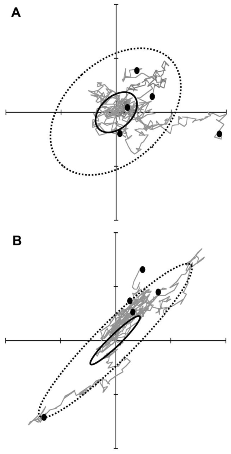
Two examples showing that the theoretical pattern of neutral divergence is proportional to the G matrix. The axes in each plot represent population mean values of two traits. A, Five simulated replicate populations share a common G matrix for two traits and have evolved independently by drift from a single common ancestor with trait values at the center of the plot. Evolution of the five populations was simulated for 1,000 generations, with final populations shown as dots. The G matrix (solid ellipse) is plotted as a 95% confidence ellipse. The five replicate populations represent a sample from a predicted probability distribution of divergence, represented by the D matrix (dashed ellipse). In this example, N_e = 100, so at t = 1,000 generations, D(t) = 10G (eq. [3]). B, Identical simulation conditions as in A, except that G has a different shape (ratio of eigenvalues), producing a different prediction for divergence, D(t).

Schluter (1996) predicted that the leading eigenvector of this divergence matrix D, representing the major direction of change among species means, would be biased toward the leading eigenvector, or principal component, of the G matrix. This prediction is based on the result that in the early stages of adaptive radiation, even in the face of selection, populations evolving toward a single fixed optimum do not necessarily evolve in the direction of greatest fitness increase on the adaptive landscape (Lande 1979, 1980b). Instead, such populations evolve in a direction close to the leading eigenvector of G, what Schluter (1996) called the genetic line of least resistance, which represents the axis of greatest genetic variation, g_max. In a purely neutral model, the major axis of divergence should align exactly with g_max (fig. 1). The other axes of variation in G also influence the direction of evolution, however, so that a multivariate distribution provides a more complete prediction of the pattern of divergence. Thus, a complete multivariate version of Schluter’s conjecture would involve comparison of all the axes of variation of the two matrices G and D, not just a comparison of their leading eigenvectors, g_max and d_max. One could accomplish this simply by testing whether G and D are proportional to each other (e.g., Blows and Higgie 2003). However, proportionality of matrices reflects similarity in two respects: ratio of eigenvalues (which we call shape) and orientation of eigenvectors (Flury 1988). Different inferences result from separate comparisons of these two aspects of matrix proportionality, hence the stepwise approach described below.

Empirical and simulation research suggests that different aspects of G evolve in different ways and in response to multiple forces (Phillips et al. 2001; Steppan et al. 2002; Jones et al. 2003, 2004, 2007). Consequently, it is useful to reparameterize G into what can be considered size, shape, and orientation parameters, as suggested by Jones et al. (2003). A symmetrical m-by-m G matrix contains m variance terms and (m² − m)/2 covariance terms, representing a total of (m² − m)/2 parameters. First, let λ₁, λ₂, and so forth, represent the eigenvalues, and let g₁, g₂, and so forth, represent the corresponding eigenvectors of G. Because G is a variance/covariance matrix, it is expected to be positive definite and therefore to have all positive real eigenvalues and orthogonal eigenvectors. Each G matrix can then be decomposed into a single size parameter

$$\mathrm{\sum }=\sum _m{\lambda }_i,$$ (5a)

a vector ε containing m − 1 shape parameters

$${\epsilon }_i=\frac{{\lambda }_i}{\mathrm{\sum }},$$ (5b)

and a vector ϕ containing (m² − m)/2 orientation parameters ϕ_i. The orientation parameters describe the angles between the eigenvectors and the trait axes, and their formulas depend on m. Note that we calculate ε_i differently from Jones et al. (2003) in order to facilitate estimation procedures and handle cases in which m > 2. Because G is a positive definite matrix, the size parameter Σ also equals the trace of G, or the sum of the genetic variances. In the case of a 2-by-2 G matrix, there is conveniently only one parameter each for size, shape, and orientation. In this two-trait case, we can represent the parameters simply as scalars (Σ, ε, and ϕ), with ϕ representing the angle between the leading eigenvector (g_max) and the axis of the first trait (Jones et al. 2003). A 2-by-2 G matrix is then parameterized as

$$\mathbf{G}=\lfloor \begin{array}{cc}\sum [\epsilon {cos}^2\varphi +(1-\epsilon ){sin}^2\varphi ]& \sum (2\epsilon -1)sin\varphi cos\varphi \\ \sum (2\epsilon -1)sin\varphi cos\varphi & \sum [\epsilon {sin}^2\varphi +(1-\epsilon ){cos}^2\varphi ]\end{array}\rfloor .$$ (6)

G is expected to change over time by neutral genetic drift in a population of finite size in the absence of natural selection. If the variance lost by fixation of alleles is replenished by a constant supply of new mutations, eventually G reaches a stable equilibrium of mutation-drift balance (Lande 1980a; Lynch and Hill 1986). This equilibrium is given by Ḡ = 2N_e M in diploid organisms, where M is the variance/covariance matrix of new mutational variation entering the population each generation (Lande 1979). If we assume that M remains constant over time, perhaps as a result of the genetic architecture of loci underlying the traits, and that G is in mutation-drift equilibrium within each taxon, then the divergence matrix is

$$\mathbf{D}(t)=\frac{\overline{\mathbf{G}}t}{{\overline{N}}_{\text{e}}}=2\mathbf{M}t.$$ (7)

In practice, both G and N_e are easier to measure in natural populations than M. If we assume mutation-drift equilibrium in a neutral model, however, we can estimate M based on these other measures. We can also reparameterize M, as we did with G. Because Ḡ is related to M by a scalar multiple, the shape and orientation parameters ε and ϕ of these two matrices are identical. The size parameters of M and G are related by

$${\mathrm{\sum }}_{\mathbf{M}}=\frac{{\mathrm{\sum }}_{\mathbf{G}}}{2{\overline{N}}_{\text{e}}},$$ (8)

where Σ_M and Σ_G are, respectively, the traces of M and G.

The Influence of Phylogeny

The trait divergence that we observe among contemporary populations is a consequence of history as well as evolutionary process. The divergence among a set of n taxa can be modeled as a sample from a multivariate normal distribution with the m-by-m variance/covariance matrix D(t) only if the taxa have evolved independently, as on a star phylogeny, with no covariance as a result of shared ancestry (as in fig. 1). This assumption of independence, however, is unrealistic in most natural situations. The effects of phylogenetic relatedness (i.e., covariance) can be removed before analysis in various ways (Felsenstein 1985; Schluter 1996; Diniz-Filho et al. 1998). Here we follow the alternative approach of Martins (1995) and include phylogenetic information directly in the calculation of the expected variance/covariance structure among taxa. Our goal then is to replace the divergence matrix D(t) with a divergence matrix that incorporates the shared history of phylogeny. We call this phylogenetic divergence matrix A.

In the case of neutral genetic drift, the variance of the probability distribution for the expected trait mean in a single taxon after t generations is given by D(t) or D(t) for single or multiple traits, respectively. Note that this variance increases linearly with time in the neutral model (eqq. [1], [3]). Now suppose that this single taxon splits at time t into two daughter taxa that evolve independently after the split. The variance of the probability distribution for each taxon’s trait mean continues to increase linearly after the split, but the means of these daughter taxa covary as a result of shared ancestry. This trait covariance remains constant after the split, and it is given simply by the variance at the time of their divergence, D(t) or D(t) (Hansen and Martins 1996). In other words, the variance of the probability distribution predicting the trait mean of the common ancestor lives on as the covariance between the daughter taxa. Note that trait correlation between the two taxa, in contrast, decreases linearly with time after cladogenesis because the variance for each daughter taxon continues to increase while the covariance between them remains constant (Martins 1995; fig. 2).

Figure 2.

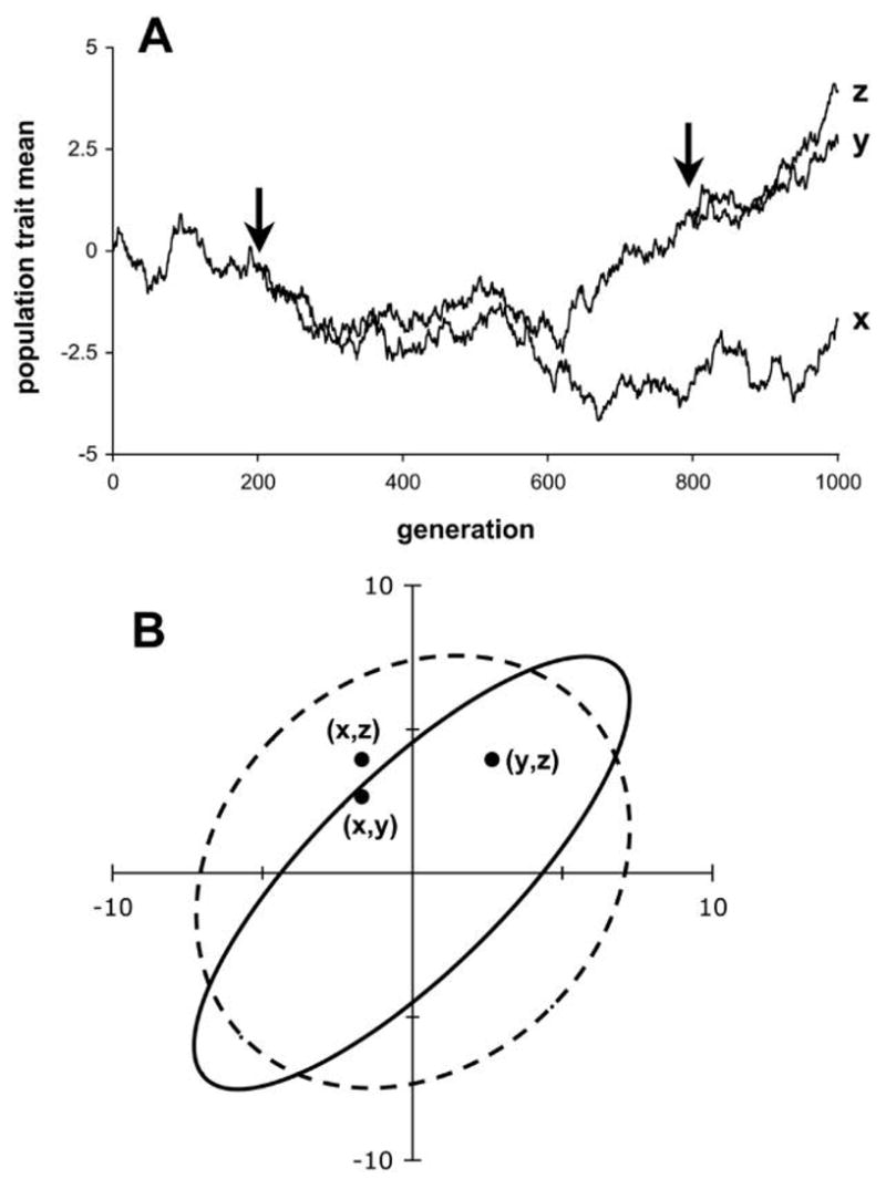
Covariance as a result of shared ancestry. A, Simulated evolution by drift of a single trait in a phylogenetic context, with speciation events at generation 200 and again at generation 800 (arrows). In this example, G = 1 and N_e = 100. B, Correlation between taxa in trait values decays after speciation. The two axes represent the values of the trait means in two taxa. The three pairs of trait means at generation 1,000 (dots) are a single sample from a trivariate normal probability distribution specified by equation (9). Expected variances and covariances of this probability distribution, calculated on the basis of the phylogeny in A and a neutral model, are shown as 95% confidence ellipses. The expected covariance between taxa y and z (solid ellipse) is relatively high because the period of common ancestry is relatively long (800 generations). In contrast, the covariance between x and y and between x and z (dashed ellipse) is relatively low because the period of common ancestry is shorter (200 generations). The variances of the distributions predicting each taxon individually are identical.

Keeping in mind this linear variance/covariance structure among related taxa, we now represent a phylogeny as a matrix of shared ancestry (Martins 1995). A phylogeny of n taxa with branch lengths can be represented by a symmetrical n-by-n matrix, which we shall call T. In this matrix, each diagonal element t_ii is the elapsed time in generations from the root of the tree to the extant taxon i, and each off-diagonal element t_ij is the time from the root to the most recent common ancestor of taxa i and j. Thus, the off-diagonal elements of T represent the elapsed time of shared ancestry for taxa i and j. Note that this formulation of a phylogeny easily accommodates both polytomies and unequal branch lengths. The latter point implies several areas of flexibility in the model: the taxa at the tips do not necessarily need to be contemporary, the phylogeny can be estimated from molecular data without assuming a molecular clock, and the conversion rate from absolute time to generations does not need to be equal across all branches. Now, for a single trait evolving by drift alone, the variance/covariance of the probability distribution of trait means at the tips of the phylogeny is given by the n-by-n matrix

$$\mathbf{A}=\frac{\overline{G}}{{\overline{N}}_{\text{e}}}\mathbf{T}=2M\mathbf{T},$$ (9)

assuming in the first case that fluctuations in G and N_e are uncorrelated with each other and that their means (arithmetic and harmonic, respectively) are equal across all branches of the phylogeny and assuming in the second case that populations are in mutation-drift equilibrium with constant mutational variance M. Each ijth element of A in equation (9) is therefore the variance term D(t_ij) from equation (1).

In the case of m traits, each element of A expands into an m-by-m block given by D(t_ij) from equation (3). Where i = j, this block gives the variance/covariance among expected trait means for taxon i. Where i ≠ j, this block gives the expected covariance among taxon means, that is, between taxon i and taxon j, for all traits (Hansen and Martins 1996). As described above, this covariance is equal to the variance/covariance for the most recent common ancestor of taxa i and j. For multiple traits, therefore, the matrix A expands into an (m × n )-by-(m × n) matrix of variance/covariance across all traits and across all taxa, incorporating both shared ancestry and the genetic covariance of traits (for further explanation, see the appendix in the online edition of the American Naturalist).

When evolution is by drift alone, the expected trait values for each taxon are equal to the trait means at the root of the phylogeny, z̄₀. Let μ be a vector of length m × n that is an n-fold concatenation of z̄₀. Thus, given a phylogeny T, ancestral trait means z̄₀, and parameters governing the drift process (Ḡ and N̄_e), the predicted probability distribution of population trait means is a multivariate normal distribution with mean vector μ and variance/covariance matrix A. Now let ζ be a vector of length m × n containing measured data—actual population means for each trait in each taxon. This vector ζ is a sample from this multivariate normal distribution. Thus, under the neutral model, the probability of producing the data ζ is given by

$$P(\mathit{\zeta })=\frac{exp[-(1/2)(\mathit{\zeta }-\mathit{\mu }{)}^{\prime }{\mathbf{A}}^{-1}(\mathit{\zeta }-\mathit{\mu })]}{\sqrt{{(2\mathit{\pi })}^{m\times n}\mid \mathbf{A}\mid }}.$$ (10)

Hypothesis Testing

ML Estimation

The foregoing specification of the outcome of evolution as a probability distribution enables us to use ML to assess the fit of the neutral model. Note that the specification of A and μ depends on the evolutionary model and a set of parameters θ. Consequently, the multivariate probability distribution in equation (10) can be transformed into a likelihood framework (Edwards 1992) in which the likelihood of a set of parameter values is

$$L(\mathit{\theta })=P(\mathit{\zeta }\mid \mathit{\theta })=P(\mathit{\zeta }\mid \mathbf{A}(\mathit{\theta }),\mathit{\mu }(\mathit{\theta })).$$ (11)

By taking the data ζ as given, we now use ML techniques to estimate parameter values in a given model that best explain the data. In the neutral model described above, these parameter values include N̄_e and the size, shape, and orientation parameters of the G matrix (Σ, ε, and ϕ, respectively). By comparing parameter estimates to independent empirical values, we can use ML to diagnose which of these parameters is responsible for a poor fit of the data to the statistical prediction given by equation (10). This identification of parameters will in turn enable us to characterize the evolutionary forces, aside from population size and genetic constraint, that have shaped the evolution of the traits. We have implemented the hypothesis-testing procedure as publicly available software called MIPoD (Hohenlohe 2007).

In general, we have two ways to estimate parameter values that maximize the likelihood of the data. One approach is to differentiate the likelihood expression, equation (11), with respect to the parameter of interest and so produce an analytical solution for the peak of the likelihood surface. When this is not practical, we must use numerical techniques to search for parameter values that maximize the likelihood expression. Below we use both techniques. As is customary, we deal mostly with the natural logarithm of the likelihood function, called log likelihood or ln L, which has the same location of maxima as does the untransformed equation (11).

We use differentiation to obtain a ML estimate for a compound parameter involving the overall size of the G matrix and effective population size. Because both Σ and N̄_e can be easily factored out of A, the log-likelihood func- tion is differentiable with respect to these parameters and can be solved explicitly for the ML estimate of Σ_G/N̄_e(=2 Σ_M for the mutation-drift equilibrium model). Unless independent information about either of these parameters is available, one cannot calculate separate ML estimates for total genetic variance and effective population size. This confounding of parameters is why many previous models contain a single Brownian motion parameter that implicitly combines total genetic variance and N_e (e.g., Hansen 1997; Butler and King 2004).

We also use differentiation to obtain a ML estimate of μ, the expected value of population trait means evolving along the observed phylogeny according to the neutral model. The ML estimate for μ in the neutral model is an n-fold concatenation of the population trait means at the root of the phylogeny, z̄₀. Assuming that these ancestral trait means will be unknown in most cases, we first produce an estimate for the ancestral trait means, ẑ₀. This ẑ₀ vector can be calculated directly by solving the set of m linear equations

$$\mathbf{S}{\widehat{\mathbf{z}}}_0=\mathbf{c},$$ (12a)

where S is an m-by-m matrix with elements

$$s_{ij}=\sum _{k=0}^{n-1}\sum _{l=0}^{n-1}{A}_{(km+i)(lm+j)}^{-1},$$ (12b)

where $A_{pq}^{-1}$ is the pqth element of the inverse matrix A⁻¹ and c is a column vector with elements

$$c_i=\sum _{l=1}^{m\times n}\lfloor {\zeta }_l\times \sum _{k=0}^{n-1}{A}_{l(km+i)}^{-1}\rfloor .$$ (12c)

Note that because both Σ and N̄_e can be factored out of A, and therefore out of A⁻¹ as well, they can also be factored out of both sides of equation (12a). Therefore, the ML solution for μ does not depend on either Σ or N̄_e, and it can be calculated independent of these parameters. In other words, the ML estimate for the expected trait means depends not on the overall rate of genetic drift but only on the shape and orientation of G and the structure of the phylogeny.

The solution for the shape and orientation parameters of the G matrix, ε and ϕ, cannot easily be found by using differentiation of the log-likelihood expression, so numerical estimation techniques must be employed. Below we use the Newton-Raphson method to find maxima on the likelihood surface (Edwards 1992). For each parameter estimate, one can also calculate approximate, marginal 95% confidence limits by finding the lower and higher values representing 1.92 log-likelihood units below the maximum while holding all other parameter values constant (Edwards 1992).

Hypothesis-Testing Hierarchy

We now turn to a hypothesis-testing framework that uses these ML estimates of Σ_G/N̄_e, ε, and ϕ to detect and diagnose departures from neutrality. The equations above describe expected outcomes under a neutral model of evolution or, more precisely, under a model of drift-mutation equilibrium, which can be considered a null model. One could simply produce a ML estimate of the complete G matrix and compare that to an independent direct estimate (e.g., calculated from measurements of traits on parents and offspring). However, most data on divergence are expected to depart from the predictions of the neutral model, so we seek to gain further insight into the kinds of roles that selection and other factors have played in producing those departures. We proceed stepwise in a hypothesis-testing hierarchy through the size, shape, and orientation parameters of G. Corresponding to each of these steps is a particular hypothesis about the evolutionary forces that have shaped trait divergence. Taken together, the steps in the hierarchy provide an overall test of the neutral model.

Our stepwise hierarchical approach is similar to the Flury hierarchy that has been used to compare multiple estimates of G (Phillips and Arnold 1999). Our approach differs from that of Phillips and Arnold (1999) in that we are comparing a direct estimate of the G matrix to one predicted from data on divergence using ML. Consequently, the statistics of comparison derive from the likelihood surface based on the neutral model. Our approach also differs in that our null hypothesis is an equality of the direct and ML estimates, while Phillips and Arnold (1999) started from a null hypothesis of G matrices with unrelated structure.

We begin by calculating the likelihood of the independent direct estimates of the G matrix parameters under the neutral model. Then at each step in the testing hierarchy, we estimate an additional parameter by ML and use a likelihood ratio test to assess whether the additional parameter significantly improves the fit of the model to the data. Significant results suggest specific ways in which evolution has deviated from the neutral prediction, thus providing information about selection (table 2). Our hierarchical approach allows us to test three basic hypotheses.

Table 2.

Hypothesis-testing hierarchy

Additional ML parameter estimate	df	Interpretation of significant LRT	Analogous step in Flury hierarchy
None	…	Null model benchmark	…
Size (Σ/N̄e)	1	Total amount of divergence either more or less than expected	Equal vs. proportional
Shape (ε)	(m − 1)	Divergence biased among axes of genetic variation	Proportional vs. full CPC
Orientation (ϕ)	(m2 − m)/2	Major axes of divergence differ from axes of genetic variation	Full CPC vs. unrelated

Note: At each step, an additional parameter underlying G matrix structure is estimated by maximum likelihood (ML), and the fit of the model is compared to the previous step by a likelihood ratio test (LRT). A significant result at each step suggests a different type of deviation from the neutral expectation. This testing procedure is somewhat analogous to the Flury hierarchy for comparing G matrices (Phillips and Arnold 1999; CPC indicates common principal components). In cases with more than two traits, the final two levels can be expanded to test individual shape and orientation parameters.

Size: Total Amount of Divergence

We begin by estimating the compound parameter Σ/by N̄_e ML, keeping the other parameters of G fixed at values of the direct estimate. We then compare the fit of the model for the ML estimate to that of the direct estimates for G and N̄_e by using a likelihood ratio test. This comparison tests the hypothesis that the total amount of divergence among taxa across all traits (i.e., the total amount of variance among observed trait means) is consistent with the neutral expectation (i.e., the variance predicted by a drift model). If we have an independent estimate of N̄_e, we can factor it out of the combined parameter and interpret the results in terms of total genetic variance Σ. If the ML estimate of Σ differs significantly from the observed value, then the total amount of divergence among taxa is either more (if Σ_obs < Σ_est) or less (if Σ_obs > Σ_est) than expected based on a model of evolution by drift alone. If we observe significantly more evolution than expected by drift, we can infer that some additional force, such as diversifying selection, has promoted divergence. Diversifying selection might take the form of a selective optimum that moves through time, for example, as ecological conditions change. Alternatively, if we observe significantly less evolution than expected by drift, we can infer that some restraining force, such as stabilizing selection, has impeded divergence. This test is the multivariate analogue of a univariate rate test of neutrality that uses the genetic variance for a single trait in conjunction with estimates of divergence, elapsed time, and effective population size (e.g., Lynch 1990; Estes and Arnold 2007).

Shape: Relative Amounts of Divergence among Axes of Variation

At the second step, we estimate both Σ and the shape parameter ε and compare the fit of the model to the previous step by using a likelihood ratio test. This comparison tests the hypothesis that the relative amount of divergence along each axis of genetic variation is consistent with the neutral expectation after removing the effects of the total amount of divergence. Under the neutral model, we expect divergence in each trait to be proportional to its genetic variance and the covariance structure of divergence among traits to be proportional to genetic covariance. In other words, we expect D and G to be proportional so that they have the same shape. Rejecting this hypothesis means that evolution has occurred faster along some axes of variation, and slower along others, than expected under neutrality. Such disparity among traits could arise if some traits or combinations of traits experience diversifying selection while others experience stabilizing selection or if trait combinations experience similar modes of selection but with different intensities. Whatever the causes of disparity among traits in the amount of evolution, disparity cannot be explained simply by differences among traits in observed genetic variance.

Because this step of the testing hierarchy examines differential rates of evolution among axes of genetic variation, there is no univariate analogue to this test. Separate univariate tests of neutrality on multiple traits would confound the total amount of evolution with the relative rates of evolution among traits. In our multivariate approach, the effect of the total amount of evolution has already been removed in the first step by estimating Σ/N̄_e. One could correct for the total amount of evolution across all traits and then conduct separate univariate tests of neutrality on the residual data. However, this approach could still miss inferences about the role of correlational selection because it would ignore the patterns of covariance among traits. In our multivariate approach, we can make inferences about correlational selection from the relative rates of evolution along the axes of genetic variation, the eigenvectors of G.

Orientation: Direction of Divergence

In the third step, we estimate all of the G matrix parameters to test the hypothesis that the major axes of divergence are congruent with the major axes of genetic variation. At this step, we ask whether the pattern of divergence and the G matrix differ in the orientation of their eigenvectors (ϕ). This comparison provides a test for Schluter’s (1996) proposition that the major axis of divergence should be biased toward the major axis of genetic variation. A rejection of the neutral model at this stage suggests either that selection has had differential impacts on the traits that do not conform to the orientation of genetic covariance or that the axes of correlational selection are not aligned with the axes of genetic variation. Because we are considering the orientation of axes in multivariate space, there is no univariate analogue to this test. In the case of two traits, a single scalar parameter ϕ establishing the orientation of g_max completely describes the orientation of G. The ML estimate of ϕ is calculated from the pattern of divergence among taxa, correcting for phylogeny under the neutral model as described above. It describes the orientation of the major axis of divergence, so it represents a phylogenetically corrected estimate of the orientation of d_max. We refer to this corrected estimate of the major axis of divergence as ${\mathbf{d}}_{max}^{\ast }$. When more than two traits are considered, it is possible to test all (m² − m)/2 parameters ϕ_i that determine the orientation of all eigenvectors of G. Because of the increase in the number of parameters and the complexity of interpretation, we will address the situation of more than two traits in more detail in a forthcoming article. Below we consider only the two-trait case.

MIPoD can also be used to compare the orientation of other matrices besides G to the pattern of divergence. In particular, if estimates of multivariate selection are available in the form of approximations to quadratic or Gaussian fitness surfaces (γ or ω matrices, respectively), their orientation can be compared with that of D (Arnold et al. 2001; Blows et al. 2004). Such a comparison is most informative when the neutral model has already been rejected on the basis of orientation (i.e., when ${\mathbf{d}}_{max}^{\ast }\ne {\mathbf{g}}_{max}$). In this situation, the orientation of the direct estimate of G does not provide an explanation for the principal axes of population differentiation, and selection becomes the leading contender. Arnold et al. (2001) have proposed that evolution may occur along a selective line of least resistance, the leading eigenvector of ω (ω_max), which may be visualized as a ridge on the Gaussian fitness surface (Phillips and Arnold 1989). This selective line of least resistance may or may not coincide with g_max. The proposition of evolution along a selective line of least resistance can be tested by comparing ω_max and ${\mathbf{d}}_{max}^{\ast }$. MIPoD implements such a comparison by holding the orientation of one eigenvector constant at the direct estimate from the adaptive landscape (which completely determines orientation in the two-trait case) and fitting the remaining parameters by ML. The likelihood of this parameter set is then compared to the best fit for all the parameter values by using a likelihood ratio test. If this test is significant, we can reject the hypothesis that the major axis of divergence aligns with the selective line of least resistance or that ${\mathbf{d}}_{max}^{\ast }$ aligns with ω_max.

Absence of Direct Parameter Estimates

Parameter separation in our hypothesis-testing framework also allows us to test aspects of the neutral model in the absence of direct estimates of parameter values. With independent estimates of both a complete G matrix and effective population size, we can test all hypotheses described above. If no independent estimate of is available, N̄_e one can produce a ML estimate of Σ_G/N̄_e(= 2Σ_M), even though one cannot test the hypothesis that total divergence is sufficiently explained by the neutral model. Nevertheless, the tests of shape and orientation can still be conducted because the effects of total divergence have been removed in the first step. Conversely, in some cases, one may have estimates of effective population size and genetic variance for each trait but no measures of genetic covariance among traits. In this case, one can test the hypothesis at the first step of the hierarchy but produce ML estimates for shape and orientation only in the latter two steps. If no independent estimates of any parameters are available, one cannot reject the neutral model in any way but can still produce ML estimates of Σ_G/N̄_e, ε, and ϕ by assuming a neutral model of evolution by drift.

Test Case

Vertebral Number in Garter Snakes

Vertebral number is remarkably constant in many vertebrate groups, apparently because deviation away from a modal number can have profoundly deleterious consequences (Galis et al. 2006). However, vertebral number in snakes is conspicuously variable among species, with means ranging from 100 to 300 total vertebrae. In garter snakes (Thamnophis), numbers of body and tail vertebrae are moderately heritable and buffered from temperature effects during development (Arnold 1988; Dohm and Garland 1993; Arnold and Phillips 1999; Arnold and Peterson 2002). Several studies indicate that selection favors an intermediate optimum number of vertebrae within populations of garter snakes and closely related genera (Arnold and Bennett 1984; Arnold 1988; Lindell et al. 1993). Other studies suggest that vertebral number differences between populations and species represent adaptations to vegetation density such that open habitats favor phenotypes with more vertebrae and brushy habitats favor phenotypes with fewer vertebrae (Kelley et al. 1997; Manier et al. 2007).

Here we examine divergence in two traits (numbers of body and tail vertebrae) in garter snakes across the genus Thamnophis (fig. 3). We used a phylogeny adapted from de Queiroz et al. (2002) that is based on mtDNA sequences. Branch lengths were converted to time in generations by using factors of 2% sequence divergence per million years (Avise 1994) and an average generation time of 5 years (Rossman et al. 1996). In those cases in which we had data on vertebral counts for multiple populations within a species, we created a new node at the midpoint of the branch leading to that species on the original tree. The data are taxon means for body and tail vertebral counts collected from a variety of sources (table A1 in the online edition of the American Naturalist and references in the appendix). In some cases, trait means were not available, and so medians or range midpoints were used as estimates of population means. Vertebral counts are usually symmetrically distributed within populations, either before or after a log transformation (Klauber 1941; Kerfoot and Kluge 1971), so such substitute estimates of the mean are reasonably reliable. Because males and females differ in vertebral number, we consider trait means and genetic variance/covariance for only females in all the analyses that follow.

Figure 3.

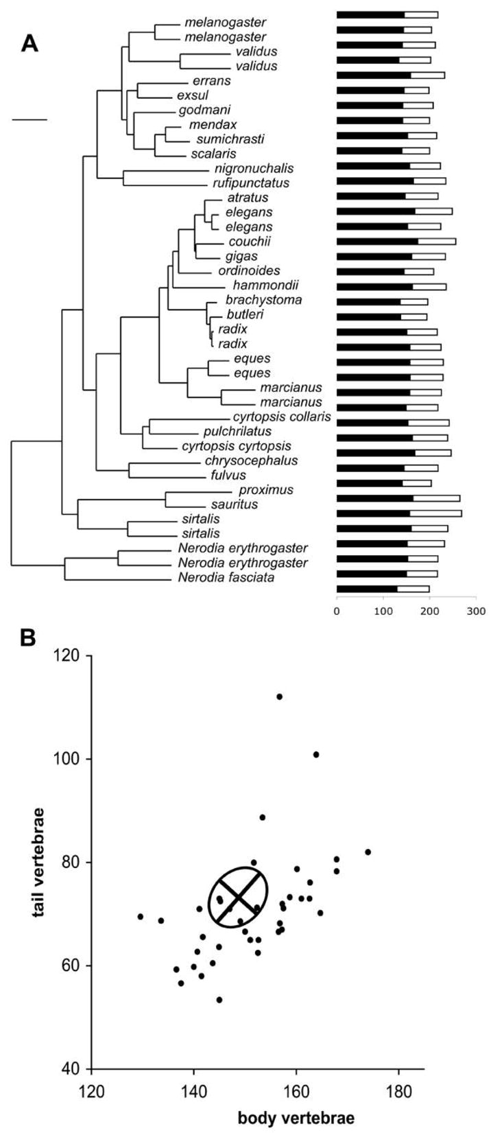
A, Evolution of body (filled bars) and tail (open bars) vertebrae in garter snakes. Phylogeny adapted from de Queiroz et al. (2002). Species are in the genus Thamnophis unless otherwise indicated. Scale bar = 2% sequence divergence in mtDNA. B, Scatterplot of trait means. The two taxa near the top of the plot are Thamnophis proximus and Thamnophis sauritus. The ellipse represents the mean G matrix from two populations of Thamnophis elegans (Arnold and Phillips 1999) and is plotted as a 95% confidence limit for within-population genetic variation, centered on the expected trait values for the data set (eqq. [12]).

We use an estimate of the G matrix for body and tail vertebral counts that represents the mean of estimates from two populations of Thamnophis elegans (Arnold and Phillips 1999; fig. 3B). To visualize a G matrix on the scale of trait values, we plot it as an ellipse with axes scaled to 1.96 times the square root of the corresponding eigenvalue; in other words, the ellipse represents a 95% confidence ellipse around the within-taxon genetic variation. The long axis of the ellipse represents g_max, the leading eigenvector of G. Additional direct estimates of G are taken individually from these two populations of T. elegans (coastal and inland, respectively; Arnold and Phillips 1999) and from a single population of Thamnophis sirtalis (Dohm and Garland 1993).

Manier and Arnold (2005) estimated effective population sizes within T. elegans from microsatellite data. Their estimates were for subpopulations within an island model metapopulation, whereas the analyses presented here consider populations with varying degrees of internal structure as single taxa. The standard island model predicts that effective population size is increased by population subdivision (Whitlock and Barton 1997). However, relaxing some of the assumptions of this model, such as equal deme size or equal reproductive output among demes, results in the observation that subdivision may often decrease rather than increase effective population size compared to census population (Whitlock and Barton 1997). This effect may be quite pronounced in some situations (e.g., Turner et al. 2006). Because the details of metapopulation dynamics in these taxa may vary (Paquin et al. 2006) and because the harmonic mean is weighted toward lower values, we use an estimate of N̄_e = 500 based on the range of values reported by Manier and Arnold (2005).

We do not have direct estimates of the selection surface based on overall fitness as a function of vertebral number for these taxa. However, two studies provide estimates of potential fitness components as a function of body and tail vertebral counts. Both studies used the method of Lande and Arnold (1983) to estimate coefficients of linear and nonlinear selection (β and γ) that describe a quadratic approximation to an individual selection surface. Arnold (1988) modeled the effects of body and tail vertebral numbers on growth rate in natural populations of female T. elegans (n = 69) by using a quadratic regression in which the vertebral numbers were standardized to unit variances. On the raw scale (i.e., without standardization to unit variances), the regression equation is relative growth (mean of one) = $-8.302+{\beta }_1{z}_1+{\beta }_2{z}_2+(1/2){\gamma }_{11}{z}_1^2+(1/2){\gamma }_{22}{z}_2^2+{\gamma }_{12}{z}_1{z}_2$, where z₁ is body and z₂ is tail. The elements of the γ matrix are γ₁₁ = −0.040 (SE = 0.012, P = .03), γ₂₂ = −0.191 (SE = 0.007, P = .01), and γ ₁₂ = 0.088 (SE = 0.068, P = .01). The estimated values for β_i were not significantly different from 0 (P > .05). Therefore, the negative inverse of γ approximates ω (Lande 1979), with ω₁₁ = −1,836.5, ω₂₂ = −384.6, and ω₁₂ = −846.2. The orientation of ω_max is given by ϕ = 0.4299. A selection surface is also available for crawling speed in neonatal Thamnophis radix (n = 143) as a function of body and tail vertebral counts (Arnold and Bennett 1988). That surface, however, was reported on log scales for both traits. We recomputed the surface by using the raw data and obtained relative burst speed (mean of one) = $1.004+{\beta }_1{z}_1+{\beta }_2{z}_2+(1/2){\gamma }_{11}{z}_1^2+(1/2){\gamma }_{22}{z}_2^2+{\gamma }_{12}{z}_1{z}_2$, with the following γ matrix: γ₁₁ = −0.002 (SE = 0.007, P > .05), γ₂₂ = −0.001 (SE = 0.010, P > .05), and γ₁₂ = 0.008 (SE = 0.003, P = .003). Again, the estimates for β_i were not significantly different from 0 (P > .05), so that ω₁₁= −16.13, ω₂₂= −32.26, and ω₁₂= −129.0. The orientation of ω_max is given by ϕ = 0.817.

Results

We used a hierarchical hypothesis-testing approach to assess the ability of a neutral drift model to explain the pattern of evolutionary divergence among Thamnophis taxa. In the first step of the hierarchy, the total genetic variance and effective population size, represented by the quotient Σ/N̄_e, determine the total dispersion of population means for the two traits in a drift model. The ML estimate for this parameter combination that best explains the data differs significantly from empirical data (fig. 4). Estimating Σ/N̄_e assuming a drift model yields combinations in which genetic variance is far too small or effective population size is far too large. When we fix N̄_e = 500, a much smaller total genetic variance better explains the data than does the direct estimate of G (P < .0001; fig. 5A; table A2 in the online edition of the American Naturalist). In other words, divergence in vertebral number is far less than expected under neutrality, suggesting that stabilizing selection—or some other restraining force—has impeded evolution. At the next step, the ML estimate for shape (ε) also better explains the data than does the direct estimate of G (P = .012). The ML estimate for ε is larger than the direct estimate, meaning a longer and narrower G matrix ellipse (fig. 5B). Divergence is biased along the axis of positive covariance between the two traits relative to the neutral prediction. In other words, we can reject the hypothesis that differences among traits in divergence are consistent with differences in genetic variances. At the third step of the hierarchy, adding the parameter estimate for orientation (ϕ) significantly improves the fit of the model (P = .001). Thus, we can reject the hypothesis that divergence occurs predominantly along the genetic line of least resistance, g_max. The estimate for ϕ is lower than the empirical value (fig. 5C), indicating that the primary axis of divergence lies closer to the axis of body vertebral count than does g_max.

Figure 4.

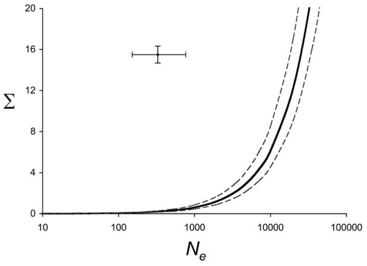
Maximum likelihood estimate (solid line) and 95% confidence limits (dashed lines) of the parameter combining total genetic variance (Σ) and effective population size (N_e), keeping shape and orientation of G fixed at the direct estimates for Thamnophis elegans (Arnold and Phillips 1999). The point estimate (cross) represents estimates in T. elegans for Σ from Arnold and Phillips (1999) and for from Manier and N_e Arnold (2005; error bars represent range of values for each parameter). The model fit is significantly better for the estimated combined parameter (likelihood ratio test; P < .0001).

Figure 5.

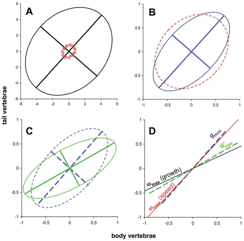
Visualization of stepwise hypothesis testing in the garter snake test case, starting from the mean G matrix for Thamnophis elegans from Arnold and Phillips (1999; see table A2 in the online edition of the American Naturalist). A, The maximum likelihood (ML) estimate for size (Σ; solid red ellipse; scaled to N̄_e = 500) with 95% confidence limits (dashed red ellipses), compared with the direct estimate of the G matrix (black ellipse). B, The ML estimate for shape (ε; blue ellipse) compared with the ML estimate from A (dashed red ellipse). Note the change in scale from A. C, The ML estimate for orientation (ϕ; green ellipse) compared with the estimate from B (dashed blue ellipse). D, Estimates of the orientation of ω_max from growth rate in T. elegans (black line) and crawling speed in Thamnophis radix (red line) plotted with the direct estimate of g_max (dashed blue line) and ${\mathbf{d}}_{max}^{\ast }$ (dashed green line).

To assess the impact of the direct estimate of the G matrix on these conclusions, we repeated the above analyses by using the estimates of G for body and tail vertebral counts from the two separate T. elegans populations (coastal and inland; Arnold and Phillips 1999) and from a population of T. sirtalis (Dohm and Garland 1993; table A2). At the first level of the hierarchy, the same result as above was obtained for all direct estimates of size (Σ) of G. In all cases, the direct estimate of Σ was significantly larger than the ML estimate (P < .0001 for all), suggesting the presence of some restraining force, such as stabilizing selection, that has impeded divergence. At the second level of the hierarchy, the results conflicted with those for the average of the T. elegans populations. The ML estimate for shape did not significantly improve the fit of the model over the direct estimate for either of the individual T. elegans populations (coastal: P = .248; inland: P = .125). In contrast, the ML estimate for shape differed significantly from the direct estimate from T. sirtalis (P = .0102), but it was smaller than the direct estimate rather than larger, as for T. elegans. In other words, the ML estimate from the divergence data produces a G matrix that is longer and narrower than the direct estimate from T. elegans but shorter and fatter than the direct estimate from T. sirtalis, when orientation is held constant at the direct estimate. Thus, the ML estimate lies within the range of variation of ε observed for these traits among Thamnophis taxa. Finally, at the third level of the hierarchy, the results were again consistent. The ML estimate for G matrix orientation was significantly smaller than the direct estimate from either of the two T. elegans populations (coastal: P < .0001; inland: P = .0009) and the direct estimate from T. sirtalis (P < .0001). For all of these direct estimates of G, we can reject the hypothesis that divergence occurs predominantly along g_max , as predicted by a drift model, and instead conclude that divergence has occurred in a direction closer to the axis of body vertebral count. Interestingly, when the orientation is shifted to the ML estimate, the ML estimate for the shape parameter becomes larger than all the direct estimates of ε. In other words, the pattern of divergence is more closely aligned with ${\mathbf{d}}_{max}^{\ast }$ relative to the second major axis of divergence, compared with the prediction from the neutral model based on any direct estimate of G. This suggests that selection has constrained divergence to a narrower band along ${\mathbf{d}}_{max}^{\ast }$ than would be predicted from the neutral model.

We also conducted the hypothesis-testing hierarchy on the average phenotypic variance-covariance matrix P, estimated from the two T. elegans populations (Arnold and Phillips 1999). The results were similar to the results for the corresponding G matrix (table A2), with significant results for size (P < .0001), shape (P = .0028), and orientation (P = .0015).

Two species, Thamnophis proximus and Thamnophis sauritus, have more tail vertebrae in relation to body vertebrae than do other garter snakes, perhaps reflecting adaptation to arboreality (fig. 3). These two species of garter snakes are more consistently found off the ground than are other species in the genus (Rossman et al. 1996). We assessed whether these taxa could be responsible for the rejection of the neutral model. Keeping effective population size fixed as above, we estimated all three parameters of the G matrix both for the full data set and for the data set with these two taxa removed (table A3 in the online edition of the American Naturalist). These two estimates of G did not differ significantly in their ability to explain the pattern of divergence in the full data set (likelihood ratio test; P = .2804).

Having rejected the hypothesis that population differentiation has occurred along a genetic line of least resistance, we ask whether ${\mathbf{d}}_{max}^{\ast }$ might align with a selective line of least resistance. Using estimates of ω_max from two studies of potential fitness components in garter snakes, we found conflicting results (fig. 5D; table A3). In the case of the growth rate surface for T. elegans, the fit of the neutral model does not differ significantly when the orientation (ϕ) is constrained to ω_max (P = .2638). We cannot reject the hypothesis that evolution has occurred along a selective line of least resistance corresponding to growth rate in this species, and, indeed, those two vectors are closely aligned (fig. 5D). However, the ML estimate does differ significantly from the orientation of ω_max from the T. radix crawling speed surface (P = .0003). Thus, we can reject the hypothesis that divergence aligns with a selective line of least resistance based on crawling speed. Note, too, that the crawling speed estimate of ω_max is closely aligned with the orientation of the direct estimate of g_max (fig. 5D). This correspondence may be a coincidence, or it may reflect evolutionary alignment of G with a persistent adaptive landscape, as predicted by simulation studies (Jones et al. 2007).

Discussion

Methodological Considerations

We have presented a statistical framework for inferring aspects of microevolutionary process from the phylogenetic pattern of trait divergence among taxa by using a neutral model of evolution. Consequently, errors can enter the framework in three places: in the data, in the model, or in the phylogeny. We consider these sources of error in turn. With respect to the data, the prediction of change in trait means over time is based on an assumption that the distribution of additive genetic variation within populations is multivariate normal (Lande 1976). Nonnormal distributions of trait values can often be transformed or rescaled to normality, and the analysis can then be performed on the transformed trait values (Lande 1976). The possibility that misleading results can be caused by only a few taxa should also be considered. Extreme values can disproportionately influence the slope of regressions (Dunn and Clarke 1987), and so they may especially influence the results of the orientation test in the last step of our testing hierarchy. One simple expedient is to determine whether the neutral model is still rejected after removing particular taxa from the data set, especially in cases where selection is known or suspected to have acted on those few taxa. In the garter snake test case, deletion of two species with exceptional ecology did not affect the conclusions (table A3). Care should be taken in interpretation, however, because statistical power to reject the neutral model may be reduced in tests of a smaller data set.

Errors arising from the neutral model enter via its central parameters, N_e and G. The most straightforward way of dealing with the effects of N_e on the conclusions is to use values that bound the probable range. The likelihood framework of MIPoD also produces confidence intervals for the compound parameter N_e/Σ that can be compared to the range of direct estimates (fig. 4). In the absence of a direct estimate, one can determine how small or large a value of N_e would have to be invoked to account for the data with a neutral model. A wildly unrealistic value for the organisms considered can provide grounds for rejecting the model. The neutral model also assumes that N̄_e (the harmonic average of effective population size across generations) is equal across all branches of the phylogeny. If this assumption is known to be violated, a correction can be applied to the phylogeny before analysis. The parameters N̄_e and t can be easily factored out of the predicted variance structure for a single population (eq. [3]) and thus factored out of each block of the phylogenetic divergence matrix A. Therefore, estimated differences among lineages in N̄_e can be incorporated by rescaling the appropriate parts of the shared ancestry matrix T. Likewise, even though direct estimates of the G matrix always come with error, Ḡ is treated as equal across branches in the model. Again, bracketing the probable values of G and using the likelihood framework to calculate confidence limits for G matrix parameters may be the best way to assess the impact of this assumption on the conclusions. If only a single direct estimate of G is available, one could compute confidence limits for elements (e.g., based on bootstrap resampling of parent-offspring data) and use those to assemble extreme estimates of G. A better approach, when multiple estimates are available, is to use those separate estimates to assess the impact on conclusions. Using this latter approach in the garter snake test case, we found that our conclusions about size and orientation were robust across the range of direct estimates of G, while the ML estimate of the shape parameter lay within the range of direct estimates when the orientation parameter was held constant.

Two perspectives on the evolutionary stability of the G matrix provide contrasting views on treating G as a constant over evolutionary time, a proposition first suggested by Lande (1975, 1979, 1980a). According to one perspective, G may fluctuate erratically through time, reflecting change in underlying gene frequencies (Turelli 1988; Shaw et al. 1995; Roff 2000) or in genes of major effect (Agrawal et al. 2001). Erratic fluctuation in G may occur especially in small populations and for traits that experience little or no stabilizing and correlational selection (Phillips et al. 2001; Whitlock et al. 2002). In such cases, using a single estimate of G, or even the average of a few estimates, in an application such as MIPoD is inadvisable because the real G is a complex time series. A second view, based on comparative studies and computer simulations, suggests conditions under which the assumption of G matrix stability may be satisfied. Comparisons of G matrices sampled from conspecific populations and related species often show that the matrices have one or more principal components in common or are even proportional (Arnold and Phillips 1999; Steppan et al. 2002). Computer simulations suggest that G matrix stability is promoted by large effective population size and mutational correlation (Jones et al. 2003). Persistent stabilizing (and correlational) selection may also produce stability in G by promoting alignment of G with the major axes of the adaptive landscape (Jones et al. 2003, 2004, 2007). A corollary expectation from this result, however, is that adaptive landscapes that have diverged in configuration may promote divergence of G among independently evolving populations.

A second cause for optimism in the use of a constant G is that even some types of fluctuations in G do not violate the assumptions required in this analysis. For example, if G is drawn independently each generation from a distribution that itself remains constant across the phylogeny, the mean of that distribution, Ḡ, provides the correct estimate of a constant G in the neutral model. Moreover, the strict assumption required here is only that Ḡ be equal across all branches of the phylogeny, so that even some short-term temporal autocorrelation of G may not substantially violate this assumption. Again, if fluctuations in G are the result of sampling from a distribution that itself remains constant, the assumption may be satisfied or nearly so. This underlying distribution could be considered to represent the genetic architecture of the traits, which shapes the M matrix of mutational variation and hence G.

Ultimately, the constancy of G over evolutionary time is an empirical question meriting further study. The advisability of using a constant estimate of Ḡ in MIPoD depends on issues that can be addressed directly by G matrix comparisons or indirectly by information about population size and modes of selection. The utility of MIPoD probably declines at larger taxonomic scales. As fundamental changes in the adaptive landscapes and genetic architecture of traits become more likely, the assumption of a constant Ḡ becomes untenable. In interpreting the results of the analysis, it is worth remembering that rejection of the neutral model can result from violations of the assumptions (e.g., constancy of Ḡ), as well as nonneutral evolution, and that nonneutral evolution itself may cause shifts in G. These should be considered as alternative interpretations of significant results.

In the absence of a direct estimate of G, one can consider using surrogates for the G matrix. The obvious candidate is the phenotypic variance-covariance matrix P. Willis et al. (1991) have described the perils of substituting P for G in equations that predict responses to selection. In the present context, however, parameter separation in our hypothesis-testing hierarchy creates a less demanding role for the P matrix. MIPoD tests whether the magnitude and pattern of population divergence are consistent with a temporally magnified version of the G matrix. To substitute P for G in this case, we must be prepared to argue that the two matrices are similar, for example, that they might be proportional (Cheverud 1988; Ackerman and Cheverud 2002). Proportional matrices share shape and orientation parameters but not size parameters. Such an argument will clearly be untenable in some circumstances. If, for example, some traits are more prone to environmental influence than are others, P will be larger than G in those trait dimensions, and the two matrices will not be proportional. In the garter snake test case, we had direct estimates of both matrices for a set of six scalation traits. P and G were indeed proportional (Arnold and Phillips 1999), perhaps because all of the traits were of a similar kind, with comparable buffering against environmental effects (Arnold and Peterson 2002). Not surprisingly, when we repeated the test case using the average P matrix for body and tail vertebral count in the two Thamnophis elegans populations (comparable to the G matrix shown in figs. 3 and 5), we obtained the same qualitative test results at all levels of the hierarchy (table A2). In this case, P may serve as a proxy for G because the two matrices are proportional.

The Kluge-Kerfoot phenomenon provides another rationale for evaluating divergence with MIPoD using P matrices. Kluge and Kerfoot (1973) argued that differences among traits in among-taxa divergence correlate with differences in within-population phenotypic variation. Unlike predictions of divergence based on G, however, this conjecture is more a description of pattern than a rigorous model of evolutionary process. Furthermore, objections to Kluge and Kerfoot’s testing procedures have been raised on a variety of statistical grounds (Sokal 1976; Rohlf et al. 1983). These objections can be circumvented by careful preliminary analysis of data, as suggested by Rohlf et al. (1983), and testing of the conjecture in MIPoD. As in the garter snake test case, a pooled or average estimate of P can be used to characterize phenotypic variation and covariation within populations. The Kluge-Kerfoot phenomenon predicts proportionality between P and D. The tests of shape and orientation in MIPoD together provide phylogenetically corrected tests of proportionality. The test of the size parameter is less relevant because it reflects the overall rate of evolution and is thus tied more directly to the process model of neutral genetic drift based on G rather than P.

Errors in the branch lengths or topology of the phylogenetic trees may also affect conclusions. Branch lengths enter the testing procedure after being calibrated to absolute time in generations. Consequently, sensitivity of results can be assessed using alternative calibrations. In the garter snake test case, we found that neutrality was so resoundingly rejected at the first testing step that calibration of branch lengths could be varied by a factor of up to 36 without affecting the conclusion. One could also test the effect of different generation times among lineages by constructing alternative matrices of shared ancestry T. Sensitivity to alternative topologies could be addressed in a similar fashion. Alternative topologies might be derived from molecular data partitions or alternative kinds of characters, alternative procedures for tree inference, or rivals under a particular criterion for tree evaluation. In any of these cases, alternative trees can be analyzed so that effects on conclusions can be assessed. In the garter snake test case, tree alternatives were not available to perform this kind of assessment.

Implicit in the testing hierarchy of MIPoD is a test of phylogenetic signal. The neutral model of drift, as a Brownian motion process, predicts a linear increase in variance over time and thus the linear relationship between shared ancestry and covariance described above. In contrast, various forms of selection cause a decay in covariance between independently evolving taxa after speciation and thus a decay of phylogenetic signal (Hansen and Martins 1996). If a data set lacks phylogenetic signal (i.e., the linear relationship between divergence and time predicted by the neutral model), MIPoD will likely reject the neutral model at one or more steps in the hierarchy. However, MIPoD may still reject the neutral model even in the face of phylogenetic signal. For instance, consider a situation in which taxa evolve toward selective optima that themselves move independently by Brownian motion (Felsenstein 1985; Estes and Arnold 2007). In this case, phylogenetic signal might be preserved, but MIPoD would likely reject the neutral model, unless the movement of optima happened to be similar to the neutral model in two further respects. First, the rate of movement of optima would have to be similar to the neutral rate of drift predicted from total genetic variation and effective population size. Second, the variance/covariance pattern of Brownian motion of optima would have to be proportional (in terms of shape and orientation) to the G matrix.

Interpretation of Results

The framework we have presented identifies a set of specific hypotheses about microevolutionary process that can be tested in a hierarchical fashion in terms of the G matrix. At the first step in the hierarchy (table 2), we test the neutral model in terms of the total amount of divergence among taxa. In the garter snake example, we rejected this aspect of the neutral model, given direct estimates of G and effective population size. Much less divergence among taxa was observed than was predicted under drift. This step is analogous to a univariate rate test of trait evolution (e.g., Lande 1977; Turelli et al. 1988; Lynch 1990). When parameterized with reasonable values for the drift process (effective population size and genetic variance), the univariate neutral prediction of divergence over time typically fails to explain observed data (Lynch 1990; Estes and Arnold 2007). Underprediction on short timescales suggests that diversifying selection has produced departures from neutrality. This result is common in studies of divergence among local populations, for example, when assessed by F_ST-Q_ST comparisons (Merilä and Crnokrak 2001; McKay and Latta 2002). On such short timescales, adaptation to spatially varying selection is often rapid, so that phenotypic divergence exceeds neutral rates. On longer timescales, however, the situation is often reversed. Here the failure of the neutral model reflects the neutral prediction that trait variance among replicate populations will increase linearly with time. In actual evolving lineages, however, divergence is rarely so extensive (Estes and Arnold 2007). Consequently, when we consider radiations of related species and genera, we find divergence to be less than expected under neutrality, as in the garter snake test case.

Such a result suggests factors that could restrain divergence and diversification. In many situations, stabilizing selection toward an intermediate optimum with restrained movement is undoubtedly the leading candidate (Hansen 1997; Estes and Arnold 2007). Other nonselective possibilities should be explored, however. Migration and hybridization, for example, can compromise the effects of diversifying selection and so might yield rates less than expected under neutrality with the assumption of independently evolving populations. Alternatively, we might hypothesize that genetic constraints limit trait divergence among taxa. The G matrix itself represents genetic constraint by describing the amount and multivariate structure of genetic variation available to evolution. Because the neutral model incorporates the G matrix in its predictions, however, to attribute failure of the neutral model to some form of genetic constraint requires some additional assumptions about process. A systematic reduction in genetic variation as divergence proceeds might produce such a limit to divergence. However, such a reduction is not supported by empirical evidence from artificial selection experiments, in which selection is typically much stronger than in nature (Hill and Caballero 1992). This hypothesis of diminished genetic variation could also be tested by gathering direct estimates of G from populations or taxa at the extremes of trait values in a radiation. If these estimates of G show a reduction in variation, particularly along axes that correspond to reduced levels of among-taxa divergence, this hypothesis could be supported.

The next two steps in our hypothesis-testing framework have no direct analogy in univariate evolution. Furthermore, they are independent of the overall rate of evolution, which was accounted for in the first step. Together, they constitute a test of proportionality between G and the divergence matrix, D. The shape test at the second step can identify combinations of traits that are evolving faster or slower than neutral expectations. Note that even if the rate test at the first step revealed an overall rate slower than expected under neutrality, some traits may nevertheless have evolved at a faster than neutral rate. Such disparities among traits can have multiple causes. Although stabilizing selection is a leading candidate cause of slower rates (Estes and Arnold 2007), in some cases other factors such as hybridization or selection limits may be at play. Likewise, rates that are accelerated relative to neutrality imply diversifying selection, but many varieties are possible. An adaptive peak may be prone to move in the trait direction that is exaggerated relative to neutral expectations. Alternatively, that trait direction might be populated by multiple peaks, with populations shifting among them. The overall significance of the shape test is that it may reveal differences among traits in selection mode and intensity.

The focus at the third step is on the direction rather than the amount (or rate) of evolution. An important prediction of the neutral model is that inheritance and population divergence will have identical axes of variation. In other words, the G and D matrices will have common principal components (i.e., identical eigenvectors). We learn more by rejecting this hypothesis than by failing to reject it. Coincidence of g_max and ${\mathbf{d}}_{max}^{\ast }$, and so on for the other eigenvectors of the two matrices, is consistent with neutrality. It also may be consistent with an early stage in adaptive radiation in which populations are far from an adaptive peak and evolving in response to selection in a direction that is biased by the G matrix, as argued by Schluter (1996). When the eigenvectors of G and D are aligned, other explanations are possible as well. For some kinds of traits, design limits and other kinds of selective constraints may produce ridges in the adaptive landscape and also predispose the adaptive peak to move in the direction of the landscape’s leading eigenvector. We call this direction the selective line of least resistance, by analogy with g_max (Arnold et al. 2001). A persistent stabilizing landscape of this kind can promote coincidence of g_max with its leading eigenvector (Jones et al. 2007) as well as coincidence of these two with ${\mathbf{d}}_{max}^{\ast }$. In other words, coincidence of g_max and ${\mathbf{d}}_{max}^{\ast }$ is consistent with a variety of scenarios, neutral and otherwise. In contrast, if we reject the hypothesis of common eigenvectors for G and D, we can certainly conclude that neutral evolution is not responsible for the direction of population diversification.

When G and D do not share common eigenvectors, as in the garter snake test case, we can ask whether the orientation of the adaptive landscape helps account for the axes of variation in divergence (i.e., the eigenvectors of D). To test this hypothesis, we need estimates of the individual selection surface, which in turn can be used to approximate the adaptive landscape. In particular, if stabilizing selection is weak, then the coefficients that describe the curvature and orientation of the individual selection surface also provide a reasonable approximation of the adaptive landscape (Lande and Arnold 1983; Phillips and Arnold 1989). Both of the approximated surfaces for garter snake data show weak curvature (i.e., small values in γ or large values in ω) and so support this assumption. In neither case, however, do the surfaces represent lifetime fitness as a function of the two vertebral counts. The two measures, crawling speed and growth rate, likely represent components of fitness but perhaps not major components. Nevertheless, the result that one of these two surfaces has an orientation that coincides with the principal axis of population divergence, in contrast with any direct estimates of G, suggests that the adaptive landscape may share some orientation with D. This possibility needs to be tested with additional selection studies. In the meantime, at least two interpretations are consistent with the shared orientation that we observed. First, all populations reside on the same adaptive landscape, with a dispersion of population means that represents a balance between drift and stabilizing selection (Lande 1976). Second, individual populations reside at or near private adaptive peaks, according to the balance of forces just described, but over evolutionary time, the peaks tend to move along a selective line of least resistance. Under this second interpretation, in the garter snake test case, this line was approximated by the estimate of from the T. elegans growth rate data. ω_max

Prospects

While G has been a player in comparative studies, its role has been surprisingly small. Nonetheless, G has been used in diverse applications that include (1) description and comparison of genetic constraints (e.g., Arnold 1992; Cheverud 1995; Steppan et al. 2002), (2) assessing the consequences of alternative schemes of directional selection (e.g., Cheverud et al. 1983), (3) retrospective analysis of selection using divergence data (Lande 1979; Price et al. 1984; Schluter 1984; Arnold 1988; Dudley 1996; Reznick et al. 1997; Jones et al. 2004), (4) estimation of generalized genetic distance (Lande 1979; Schluter 1984), (5) testing for evolution along genetic lines of least resistance (Schluter 1996), and (6) testing for proportionality between G and matrices of population divergence (Lofsvold 1988; Blows and Higgie 2003; Bégin and Roff 2004; McGuigan et al. 2005). Despite these applications, G has not been used in a variety of other circumstances in which it is likely to supply critical information. For example, so far as we know, G has not been used to (1) weight characters in the inference of phylogenetic trees (but see Schaffer 1986), (2) model trait evolution on phylogenies, or (3) reconstruct ancestral character states. In some cases in which G might be used, it figures in the formulation of methodology but plays no role in actual tests (Martins and Hansen 1996, 1997). In other cases, G plays a cryptic role, hidden within a compound parameter that is used to represent the combined effects of finite population size, genetic constraints, and stabilizing selection (Hansen 1997; Butler and King 2004). Parameterizations that separate these diverse contributions have multiple advantages. By using models with explicit, separate terms for inheritance, selection, and population size, one can determine whether each of these factors takes realistic values (Estes and Arnold 2007). In addition, by using such an approach in MIPoD, one can directly incorporate information about population size and genetic constraints into the analysis of divergence data.

Looking to the future, we can ask what could be gained by using the G matrix in the methodologies of comparative study. A grand hope is that we might be able to deduce the modes and patterns of selection that drive adaptive radiations. By using the G matrix in our comparative methods, we should be able to separate the effects of genetic constraint from those of selection. The most powerful format for accomplishing this separation is the family of stochastic models developed by Lande and associates to describe population differentiation during neutral or adaptive radiations (Lande 1976, 1985, 1986; Hansen and Martins 1996; Lande and Shannon 1996). The neutral model that we have used in MIPoD is the simplest basal member of the family. Models that incorporate selection are usually cast in terms of an adaptive landscape with a peak that is stationary or that moves in any of a variety of ways. A generalization emerging from the models that have been developed so far is that the G matrix affects differentiation during the early stages of a radiation, but its influence decays through time exponentially (Hansen and Martins 1996; Schluter 1996; Estes and Arnold 2007). Exceptions are found in certain kinds of landscapes, namely, those in which the peak moves systematically, for example, in a progressive fashion (e.g., Lynch and Lande 1995; Jones et al. 2004). If the peak moves randomly (e.g., as in Brownian or white noise motion), so that there is no change in average position over time, the influence of G decays over time (Hansen and Martins 1996). Thus, the separation that we hope for in resolving the roles of constraint and selection occurs naturally in some kinds of adaptive landscape models, assuming that we do our analysis on the right timescale. In situations in which the movement of adaptive peaks includes a systematic component, we will need to use G to fully characterize the role of selection.

Literature Cited

- Ackerman R, Cheverud J. Discerning evolutionary processes in patterns of tamarin (genus Saguinus) craniofacial variation. American Journal of Physical Anthropology. 2002;117:260–271. doi: 10.1002/ajpa.10038. [DOI] [PubMed] [Google Scholar]
- Agrawal AF, Brodie ED, III, Rieseberg LH. Possible consequences of genes of major effect: transient changes in the G matrix. Genetica. 2001;112–113:33–43. [PubMed] [Google Scholar]
- Arnold SJ. Quantitative genetics and selection in natural populations: microevolution of vertebral numbers in the garter snake Thamnophis elegans. In: Weir BS, Eisen EJ, Goodman MM, Namkoong G, editors. Proceedings of the Second International Conference on Quantitative Genetics; Sinauer, Sunderland, MA. 1988. pp. 619–636. [Google Scholar]
- Arnold SJ. Constraints on phenotypic evolution. American Naturalist. 1992;140(suppl):S85–S107. doi: 10.1086/285398. [DOI] [PubMed] [Google Scholar]
- Arnold SJ, Bennett AF. Behavioural variation in natural populations. III. Antipredator displays in the garter snake Thamnophis radix. Animal Behaviour. 1984;32:1108–1118. [Google Scholar]
- Arnold SJ, Bennett AF. Behavioural variation in natural populations. V. Morphological correlates of locomotion in the garter snake Thamnophis radix. Biological Journal of the Linnean Society. 1988;34:175–190. [Google Scholar]
- Arnold SJ, Peterson CR. A model for optimal reaction norms: the case of the pregnant garter snake and her temperature-sensitive embryos. American Naturalist. 2002;160:306–316. doi: 10.1086/341522. [DOI] [PubMed] [Google Scholar]
- Arnold SJ, Phillips PC. Hierarchical comparison of genetic variance-covariance matrices. II. Coastal-inland divergence in the garter snake, Thamnophis elegans. Evolution. 1999;53:1516–1527. doi: 10.1111/j.1558-5646.1999.tb05415.x. [DOI] [PubMed] [Google Scholar]
- Arnold SJ, Pfrender ME, Jones AG. The adaptive landscape as a conceptual bridge between micro- and macroevolution. Genetica. 2001;112–113:9–32. [PubMed] [Google Scholar]
- Avise JC. Molecular markers, natural history and evolution. Chapman & Hall; New York: 1994. [Google Scholar]
- Baum DA, Donoghue MJ. A likelihood framework for the phylogenetic analysis of adaptation. In: Orzack SH, Sober E, editors. Adaptationism and optimality. Cambridge University Press; Cambridge: 2001. pp. 24–44. [Google Scholar]
- Bégin M, Roff DA. From micro- to macroevolution through quantitative genetic variation: positive evidence from field crickets. Evolution. 2004;58:2287–2304. doi: 10.1111/j.0014-3820.2004.tb01604.x. [DOI] [PubMed] [Google Scholar]
- Blows MW. A tale of two matrices: multivariate approaches in evolutionary biology. Journal of Evolutionary Biology. 2007;20:1–8. doi: 10.1111/j.1420-9101.2006.01164.x. [DOI] [PubMed] [Google Scholar]
- Blows MW, Higgie M. Genetic constraints on the evolution of mate recognition under natural selection. American Naturalist. 2003;161:240–253. doi: 10.1086/345783. [DOI] [PubMed] [Google Scholar]
- Blows MW, Chenoweth SF, Hine E. Orientation of the genetic variance-covariance matrix and the fitness surface for multiple male sexually selected traits. American Naturalist. 2004;163:329–340. doi: 10.1086/381941. [DOI] [PubMed] [Google Scholar]
- Butler MA, King AA. Phylogenetic comparative analysis: a modeling approach for adaptive evolution. American Naturalist. 2004;164:683–695. doi: 10.1086/426002. [DOI] [PubMed] [Google Scholar]
- Carvalho P, Diniz-Filho JAF, Bini LM. The impact of Felsenstein’s “Phylogenies and the comparative method” on evolutionary biology. Scientometrics. 2005;62:53–66. [Google Scholar]
- Charlesworth B. The cost of phenotypic evolution. Paleobiology. 1984;10:319–327. [Google Scholar]
- Cheverud J. A comparison of phenotypic and genetic correlations. American Naturalist. 1988;42:958–968. doi: 10.1111/j.1558-5646.1988.tb02514.x. [DOI] [PubMed] [Google Scholar]
- Cheverud J. Morphological integration in the saddle-back tamarin (Saguinus fuscicollis) cranium. American Naturalist. 1995;145:63–89. [Google Scholar]
- Cheverud J, Rutledge JJ, Atchley WR. Quantitative genetics of development: genetic correlations among age-specific trait values and the evolution of ontogeny. Evolution. 1983;37:895–905. doi: 10.1111/j.1558-5646.1983.tb05619.x. [DOI] [PubMed] [Google Scholar]
- Darst CR, Menendez-Guerrero PA, Coloma LA, Cannatella DC. Evolution of dietary specialization and chemical defense in poison frogs (Dendrobatidae): a comparative analysis. American Naturalist. 2005;165:56–69. doi: 10.1086/426599. [DOI] [PubMed] [Google Scholar]
- de Queiroz A, Lawson R, Lemos-Espinal JA. Phylogenetic relationships of North American garter snakes (Thamnophis) based on four mitochondrial genes: how much DNA sequence is enough? Molecular Phylogenetics and Evolution. 2002;22:315–329. doi: 10.1006/mpev.2001.1074. [DOI] [PubMed] [Google Scholar]
- Diniz-Filho JAF, De Sant’ana CER, Bini LM. An eigenvector method for estimating phylogenetic inertia. Evolution. 1998;52:1247–1262. doi: 10.1111/j.1558-5646.1998.tb02006.x. [DOI] [PubMed] [Google Scholar]
- Dohm MR, Garland TJ., Jr Quantitative genetics of scale counts in the garter snake Thamnophis sirtalis. Copeia. 1993;1993:987–1002. [Google Scholar]
- Dudley SA. The response to differing selection on plant physiological traits: evidence for local adaptation. Evolution. 1996;50:103–110. doi: 10.1111/j.1558-5646.1996.tb04476.x. [DOI] [PubMed] [Google Scholar]
- Dunn OJ, Clarke VA. Applied statistics: analysis of variance and regression. Wiley; New York: 1987. [Google Scholar]
- Edwards AWF. Likelihood. Johns Hopkins University Press; Baltimore: 1992. [Google Scholar]
- Estes S, Arnold SJ. Resolving the paradox of stasis: models with stabilizing selection explain evolutionary divergence on all timescales. American Naturalist. 2007;169:227–244. doi: 10.1086/510633. [DOI] [PubMed] [Google Scholar]
- Felsenstein J. Phylogenies and the comparative method. American Naturalist. 1985;125:1–15. doi: 10.1086/703055. [DOI] [PubMed] [Google Scholar]
- Flury BD. Common principal components and related multivariate models. Wiley; New York: 1988. [Google Scholar]
- Galis F, van Dooren TJM, Feuth JD, Metz JAJ, Witkam A, Ruinard S, Steinenga MJ, Wijnaendts LCD. Extreme selection in humans against homeotic transformations of cervical vertebrae. Evolution. 2006;60:2643–2654. [PubMed] [Google Scholar]
- Hansen TF. Stabilizing selection and the comparative analysis of adaptation. Evolution. 1997;51:1341–1351. doi: 10.1111/j.1558-5646.1997.tb01457.x. [DOI] [PubMed] [Google Scholar]
- Hansen TF, Houle D. Evolvability, stabilizing selection, and the problem of stasis. In: Pigliucci M, Preston K, editors. Phenotypic integration. Oxford University Press; Oxford: 2004. pp. 130–150. [Google Scholar]
- Hansen TF, Martins EP. Translating between microevolutionary process and macroevolutionary patterns: the correlation structure of interspecific data. Evolution. 1996;50:1404–1417. doi: 10.1111/j.1558-5646.1996.tb03914.x. [DOI] [PubMed] [Google Scholar]
- Harvey PH, Pagel MD. The comparative method in evolutionary biology. Oxford University Press; Oxford: 1991. [Google Scholar]
- Hill WG, Caballero A. Artificial selection experiments. Annual Review of Ecology and Systematics. 1992;23:287–310. [Google Scholar]
- Hohenlohe PA. MIPoD: Microevolutionary inference from patterns of divergence. 2007 doi: 10.1086/527498. Software available at http://www.oregonstate.edu/~hohenlop. [DOI] [PMC free article] [PubMed]
- Hunt G. Evolutionary divergence in directions of high phenotypic variance in the ostracode genus Poseidonamicus. Evolution. 2007;61:1560–1576. doi: 10.1111/j.1558-5646.2007.00129.x. [DOI] [PubMed] [Google Scholar]
- Jones AG, Arnold SJ, Bürger R. Stability of the G matrix in a population experiencing pleiotropic mutation, stabilizing selection, and genetic drift. Evolution. 2003;57:1747–1760. doi: 10.1111/j.0014-3820.2003.tb00583.x. [DOI] [PubMed] [Google Scholar]
- Jones AG, Arnold SJ, Bürger R. Evolution and stability of the G matrix on a landscape with a moving optimum. Evolution. 2004;58:1639–1654. doi: 10.1111/j.0014-3820.2004.tb00450.x. [DOI] [PubMed] [Google Scholar]
- Jones AG, Arnold SJ, Bürger R. The mutation matrix and the evolution of evolvability. Evolution. 2007;61:727–745. doi: 10.1111/j.1558-5646.2007.00071.x. [DOI] [PubMed] [Google Scholar]
- Kelley KC, Arnold SJ, Gladstone J. The effects of substrate and vertebral number on locomotion in the garter snake Thamnophis elegans. Functional Ecology. 1997;11:189–198. [Google Scholar]
- Kerfoot WC, Kluge AG. Impact of the lognormal distribution on studies of phenotypic variation and evolutionary rates. Systematic Zoology. 1971;20:459–464. [Google Scholar]
- Kingsolver JG, Hoekstra HE, Hoekstra JM, Berrigan D, Vignieri SN, Hill CE, Hoang A, Gilbert P, Beerli P. The strength of phenotypic selection in natural populations. American Naturalist. 2001;157:245–261. doi: 10.1086/319193. [DOI] [PubMed] [Google Scholar]
- Klauber LM. The frequency distribution of certain herpetological variables. Bulletin of the Zoological Society of San Diego. 1941;17:5–31. [Google Scholar]
- Kluge AG, Kerfoot WC. The predictability and regularity of character divergence. American Naturalist. 1973;107:426–442. [Google Scholar]
- Lande R. The maintenance of genetic variability by mutation in a polygenic character with linked loci. Genetical Research. 1975;26:221–235. doi: 10.1017/s0016672300016037. [DOI] [PubMed] [Google Scholar]
- Lande R. Natural selection and random genetic drift in phenotypic evolution. Evolution. 1976;30:314–334. doi: 10.1111/j.1558-5646.1976.tb00911.x. [DOI] [PubMed] [Google Scholar]
- Lande R. Statistical tests for natural selection on quantitative characters. Evolution. 1977;31:442–444. doi: 10.1111/j.1558-5646.1977.tb01025.x. [DOI] [PubMed] [Google Scholar]
- Lande R. Quantitative genetic analysis of multivariate evolution applied to brain : body allometry. Evolution. 1979;33:402–416. doi: 10.1111/j.1558-5646.1979.tb04694.x. [DOI] [PubMed] [Google Scholar]
- Lande R. The genetic covariance between characters maintained by pleiotropic mutation. Genetics. 1980a;94:203–215. doi: 10.1093/genetics/94.1.203. [DOI] [PMC free article] [PubMed] [Google Scholar]
- Lande R. Sexual dimorphism, sexual selection, and adaptation in polygenic characters. Evolution. 1980b;34:292–305. doi: 10.1111/j.1558-5646.1980.tb04817.x. [DOI] [PubMed] [Google Scholar]
- Lande R. Expected time for random genetic drift of a population between stable phenotypic states. Proceedings of the National Academy of Sciences of the USA. 1985;82:7641–7645. doi: 10.1073/pnas.82.22.7641. [DOI] [PMC free article] [PubMed] [Google Scholar]
- Lande R. The dynamics of peak shifts and the pattern of morphological evolution. Paleobiology. 1986;12:343–354. [Google Scholar]
- Lande R, Arnold SJ. The measurement of selection on correlated characters. Evolution. 1983;37:1210–1226. doi: 10.1111/j.1558-5646.1983.tb00236.x. [DOI] [PubMed] [Google Scholar]
- Lande R, Shannon S. The role of genetic variation in adaptation and population persistence in a changing environment. Evolution. 1996;50:434–437. doi: 10.1111/j.1558-5646.1996.tb04504.x. [DOI] [PubMed] [Google Scholar]
- Lindell LE, Forsman A, Merila J. Variation in number of ventral scales in snakes: effects of body size, growth rate and survival in the adder Vipera berus. Journal of Zoology (London) 1993;230:101–115. [Google Scholar]
- Lofsvold D. Quantitative genetics of morphological differentiation in Peromyscus. II. Analysis of selection and drift. Evolution. 1988;42:54–67. doi: 10.1111/j.1558-5646.1988.tb04107.x. [DOI] [PubMed] [Google Scholar]
- Lynch M. The rate of morphological evolution in mammals from the standpoint of the neutral expectation. American Naturalist. 1990;136:727–741. [Google Scholar]
- Lynch M. Methods for the analysis of comparative data in evolutionary biology. Evolution. 1991;45:1065–1080. doi: 10.1111/j.1558-5646.1991.tb04375.x. [DOI] [PubMed] [Google Scholar]
- Lynch M, Hill WG. Phenotypic evolution by neutral mutation. Evolution. 1986;40:915–935. doi: 10.1111/j.1558-5646.1986.tb00561.x. [DOI] [PubMed] [Google Scholar]
- Lynch M, Lande R. Evolution and extinction in response to environmental change. In: Kareiva PM, Kingsolver JG, Huey RB, editors. Biotic interactions and global change. Sinauer; Sunderland, MA: 1995. pp. 234–250. [Google Scholar]
- Lynch M, Pfrender ME, Spitze K, Lehman N, Hicks J, Allen D, Latta L, Ottene M, Bogue F, Colbourne J. The quantitative and molecular genetic architecture of a subdivided species. Evolution. 1999;53:100–110. doi: 10.1111/j.1558-5646.1999.tb05336.x. [DOI] [PubMed] [Google Scholar]
- Manier MK, Arnold SJ. Population genetic analysis identifies source-sink dynamics for two sympatric garter snake species (Thamnophis elegans and Thamnophis sirtalis) Molecular Ecology. 2005;14:3965–3976. doi: 10.1111/j.1365-294X.2005.02734.x. [DOI] [PubMed] [Google Scholar]
- Manier MK, Seyler CM, Arnold SJ. Adaptive divergence within and between ecotypes of the terrestrial garter snake, Thamnophis elegans, assessed with comparisons FST-QST. Journal of Evolutionary Biology. 2007;20:1705–1719. doi: 10.1111/j.1420-9101.2007.01401.x. [DOI] [PubMed] [Google Scholar]
- Martins EP. Estimating the rate of phenotypic evolution from comparative data. American Naturalist. 1994;144:193–209. [Google Scholar]
- Martins EP. Phylogenies and comparative data, a microevolutionary perspective. Philosophical Transactions of the Royal Society B: Biological Sciences. 1995;349:85–91. doi: 10.1098/rstb.1995.0094. [DOI] [PubMed] [Google Scholar]
- Martins EP. Adaptation and the comparative method. Trends in Ecology & Evolution. 2000;15:296–299. doi: 10.1016/s0169-5347(00)01880-2. [DOI] [PubMed] [Google Scholar]
- Martins EP, Garland TJ., Jr Phylogenetic analyses of the correlated evolution of continuous characters: a simulation study. Evolution. 1991;45:534–557. doi: 10.1111/j.1558-5646.1991.tb04328.x. [DOI] [PubMed] [Google Scholar]
- Martins EP, Hansen TF. A microevolutionary link between phylogenies and comparative data. In: Harvey P, Maynard Smith J, Leigh-Brown A, editors. New uses for new phylogenies. Oxford University Press; Oxford: 1996. pp. 273–288. [Google Scholar]
- Martins EP, Hansen TF. Phylogenies and the comparative method: a general approach to incorporating phylogenetic information into the analysis of interspecific data. American Naturalist. 1997;149:646–667. [Google Scholar]
- McGuigan K, Chenoweth SF, Blows MW. Phenotypic divergence along lines of genetic variance. American Naturalist. 2005;165:32–43. doi: 10.1086/426600. [DOI] [PubMed] [Google Scholar]
- McKay JK, Latta RG. Adaptive population divergence: markers, QTL and traits. Trends in Ecology & Evolution. 2002;17:285–291. [Google Scholar]
- Merilä J, Crnokrak P. Comparison of genetic differentiation at marker loci and quantitative traits. Journal of Evolutionary Biology. 2001;14:892–903. [Google Scholar]
- Mousseau TA, Roff DA. Natural selection and the heritability of fitness components. Heredity. 1987;59:181–197. doi: 10.1038/hdy.1987.113. [DOI] [PubMed] [Google Scholar]
- Ord TJ, Martins EP. Tracing the origins of signal diversity in anole lizards: phylogenetic approaches to inferring the evolution of complex behaviour. Animal Behaviour. 2006;71:1411–1429. [Google Scholar]
- Paquin MM, Wylie GD, Routman EJ. Population structure of the giant garter snake, Thamnophis gigas. Conservation Genetics. 2006;7:25–36. [Google Scholar]
- Phillips PC, Arnold SJ. Visualizing multivariate selection. Evolution. 1989;43:1209–1222. doi: 10.1111/j.1558-5646.1989.tb02569.x. [DOI] [PubMed] [Google Scholar]
- Phillips PC, Arnold SJ. Hierarchical comparison of genetic variance-covariance matrices. I. Using the Flury hierarchy. Evolution. 1999;53:1506–1515. doi: 10.1111/j.1558-5646.1999.tb05414.x. [DOI] [PubMed] [Google Scholar]
- Phillips PC, Whitlock MC, Fowler K. Inbreeding changes the shape of the genetic covariance matrix in Drosophila melanogaster. Genetics. 2001;158:1137–1145. doi: 10.1093/genetics/158.3.1137. [DOI] [PMC free article] [PubMed] [Google Scholar]
- Price TD, Grant PR, Boag PT. Genetic changes in the morphological differentiation of Darwin’s ground finches. In: Wohrmann K, Loeschke V, editors. Population biology and evolution. Springer; Berlin: 1984. pp. 49–66. [Google Scholar]
- Reznick DN, Shaw FH, Rodd FH, Shaw RG. Evaluation of the rate of evolution in natural populations of guppies (Poecilia reticulata) Science. 1997;275:1934–1937. doi: 10.1126/science.275.5308.1934. [DOI] [PubMed] [Google Scholar]
- Roff DA. The evolution of the G matrix: selection or drift? Heredity. 2000;84:135–142. doi: 10.1046/j.1365-2540.2000.00695.x. [DOI] [PubMed] [Google Scholar]
- Rohlf FJ. Comparative methods for the analysis of continuous variables: geometric interpretations. Evolution. 2001;55:2143–2160. doi: 10.1111/j.0014-3820.2001.tb00731.x. [DOI] [PubMed] [Google Scholar]
- Rohlf FJ, Gilmartin AJ, Hart G. The Kluge-Kerfoot phenomenon: a statistical artifact. Evolution. 1983;37:180–202. doi: 10.1111/j.1558-5646.1983.tb05526.x. [DOI] [PubMed] [Google Scholar]
- Rossman DA, Ford NB, Seigel RA. The garter snakes: evolution and ecology. University of Oklahoma Press; Norman: 1996. [Google Scholar]
- Schaffer HB. The utility of quantitative genetic parameter estimates in character weighting. Systematic Zoology. 1986;35:124–134. [Google Scholar]
- Schluter D. Morphological and phylogenetic relations among the Darwin’s finches. Evolution. 1984;38:921–930. doi: 10.1111/j.1558-5646.1984.tb00363.x. [DOI] [PubMed] [Google Scholar]
- Schluter D. Adaptive radiation along genetic lines of least resistance. Evolution. 1996;50:1766–1774. doi: 10.1111/j.1558-5646.1996.tb03563.x. [DOI] [PubMed] [Google Scholar]
- Shaw FH, Shaw RG, Wilkinson GS, Turelli M. Changes in genetic variances and covariances: G whiz! Evolution. 1995;49:1260–1267. doi: 10.1111/j.1558-5646.1995.tb04452.x. [DOI] [PubMed] [Google Scholar]
- Sokal RR. The Kluge-Kerfoot phenomenon reexamined. American Naturalist. 1976;110:1077–1092. [Google Scholar]
- Steppan SJ. Phylogenetic comparative analysis of multivariate data. In: Pigliucci M, Preston K, editors. Phenotypic integration. Oxford University Press; Oxford: 2004. pp. 325–344. [Google Scholar]
- Steppan SJ, Phillips PC, Houle D. Comparative quantitative genetics: evolution of the G matrix. Trends in Ecology & Evolution. 2002;17:320–327. [Google Scholar]
- Strmberg CAE. Evolution of hypsodonty in equids: testing a hypothesis of adaptation. Paleobiology. 2006;32:236–258. [Google Scholar]
- Turelli M. Phenotypic evolution, constant covariances, and the maintenance of additive variation. Evolution. 1988;42:1342–1347. doi: 10.1111/j.1558-5646.1988.tb04193.x. [DOI] [PubMed] [Google Scholar]
- Turelli M, Gillespie JH, Lande R. Rate tests for selection on quantitative characters during macroevolution and microevolution. Evolution. 1988;42:1085–1089. doi: 10.1111/j.1558-5646.1988.tb02526.x. [DOI] [PubMed] [Google Scholar]
- Turner TF, Osborne MJ, Moyer GR, Benavides MA, Alo D. Life history and environmental variation interact to determine effective population to census size ratio. Proceedings of the Royal Society B: Biological Sciences. 2006;273:3065–3073. doi: 10.1098/rspb.2006.3677. [DOI] [PMC free article] [PubMed] [Google Scholar]
- Whitlock MC, Barton NH. The effective size of a subdivided population. Genetics. 1997;146:427–441. doi: 10.1093/genetics/146.1.427. [DOI] [PMC free article] [PubMed] [Google Scholar]
- Whitlock MC, Phillips PC, Fowler K. Persistence of changes in the genetic covariance matrix after a bottleneck. Evolution. 2002;56:1968–1975. doi: 10.1111/j.0014-3820.2002.tb00122.x. [DOI] [PubMed] [Google Scholar]
- Willis JH, Coyne JA, Kirkpatrick M. Can one predict the evolution of quantitative characters without genetics? Evolution. 1991;45:441–444. doi: 10.1111/j.1558-5646.1991.tb04418.x. [DOI] [PubMed] [Google Scholar]
Associated Data
This section collects any data citations, data availability statements, or supplementary materials included in this article.