

Abstract
The presence of native contacts in the denatured state of many proteins suggests that elements of the biologically active structure of these molecules are formed during the initial stage of the folding process. The rapidity with which these events take place makes it difficult to study them in vitro, but, by the same token, suitable for studies in silico. With the help of all-atom, explicit solvent, molecular dynamics simulations we have followed in time, starting from elongated structureless conformations, the early events in the folding of src-SH3 domain and of proteins G, L, and CI2. It is observed that within the first 50 ns two important events take place, essentially independent of each other: hydrophobic collapse and formation of a few selected native contacts. The same contacts are also found in simulations carried out in the presence of guanidinium chloride in order to reproduce the conditions used to characterize experimentally the denatured state and testify to the fact that these contacts are to be considered a resilient characterizing property of the denaturated state.
Keywords: protein structure/folding, molecular mechanics/dynamics
The early events of protein folding are difficult to access experimentally because of instrumental limitations (Ferguson and Fersht 2003). The dead time of typical stopped-flow experiments is of the order of 500 μs, which may be reduced to ∼100 ns by means of temperature jump methods (Fersht 1999). In addition to these time resolution limitations, one is also confronted with the fact that fast detection techniques (such as fluorescence spectroscopy) needed in ultrafast experiments, can only measure gross features of protein structure.
To obtain structural information at atomic detail one needs to make use of techniques like nuclear magnetic resonance (NMR), which, being less sensitive than optical techniques, need longer acquisition times. Consequently, NMR experiments are only able to characterize very long-lived states of the protein, such as the denatured state (stabilized by chemicals like urea, guanidinium chloride, or acids). Such an approach has provided evidence for the presence, in a number of proteins, of residual structures in the denatured state (Shortle 1996; Mok at al. 1999; Yi et atl. 2000; Navon at al. 2001), although under conditions which are different from biological conditions in which folding takes place. It is sensible to conjecture that such structuring is, to some extent, associated with the folding mechanism of the protein, driving the protein toward its native state, thus helping to solve Levinthal's paradox. The study of simplified models, although not providing molecular details, suggests that this is indeed the case (Broglia and Tiana 2001; Broglia et al. 2004, 2006).
The time needed for the formation of the residual structure during renaturation is not known. FRET experiments on BLL have shown that the fastest event, an overall collapse of the chain, takes place in 60 ns, while the formation of secondary structures is several orders of magnitude slower (Sadqui et al. 2003). It is, however, possible that residual structure does not correspond to elements of secondary structures, but to small parts of them or to turns that are hardly detected by the experimental techniques mentioned above.
Another approach to study the initial events in protein folding is to employ molecular dynamics (MD) simulations with detailed all-atom models in explicit solvent, that is, models that carefully account for the physical and chemical properties of amino acids. The limitations of this approach lie in the fact that simulating long periods of time is computationally expensive. The price is, however, affordable if one limits the study to the very first stages of the folding process. So far, MD simulations have been mainly used to investigate the unfolding of small proteins at high temperature. Exceptions are the massive simulation of the folding of the villin headpiece by Duan and Kollman (1998) and by Pande and coworkers (Shirts and Pande 2000). These calculations are anyway focused on characterizing the native state without any prior knowledge of its conformation.
While a computational characterization of the thermodynamics of the denatured state of even small proteins is presently out of reach because of the highly entropic character of this state, the study of the early events of protein folding is within the limits of current MD simulations. In the following we shall present results of a study of the first 50 ns of the kinetics of four small proteins, starting from an elongated, structureless conformation. Each simulation is replicated thrice, focusing the attention on the events (like more or less pronounced collapse, formation of specific contacts, etc.) which take place in all the replicas. We shall conclude that each of the proteins studied displays some local native contacts formed very early in the folding process and present afterward throughout the simulations. Of note is the fact that these results are not inconsistent with experimental information concerning the folding of these proteins, in particular with that concerning the structure of the transition state ensemble. In fact, the transition states of the four proteins studied in this work were exhaustively characterized by means of φ-value analysis (Fersht 1999; Riddle et al. 1999; McAllister et al. 2000; Kazmirski et al. 2001). All of them are associated with the formation of specific structures, although displaying different extension and stability (more diffuse and less stable for CI2, more localized and stable for the other three). As discussed below, most of the early-formed native contacts we observe in the simulations (with the exception of SH3) belong to the regions of the protein structured in the transition state.
Results
Structure of the collapsed state
The dynamics of protein G, protein L, SH3, and CI2 was followed for 50 ns along three trajectories starting from elongated, structureless initial conformations. These conformations have been produced to avoid any bias toward the formation of contacts, although most likely their statistical weight is very low. During the first 20 ns of each run, all of the four proteins studied experience a collapse toward a compact state. The radius of gyration Rg of the Cα atoms for the three runs of SH3 is shown in Figure 1. It is seen that Rg changes from a value of 2.2 nm (extended structure) to 1.3 nm (collapsed situation). As a reference, the value of Rg corresponding to the native conformation is 0.96 nm. The difference in the value of Rg associated with the collapsed situation and that of the states reached by SH3 after 50 ns is less than 1 Å (=[1.3–1.2] nm ∼ 0.1 nm).
Figure 1.

Radius of gyration and, in the inset, RMSD of SH3-src for the three simulations (displayed, respectively, with solid curve, dashed curve, and dot-dashed curve).
The RMSD of the Cα as a function of time is shown in the inset of Figure 1. In the timescale of the hydrophobic collapse, the value of the RMSD of the different trajectories converges to 1.2 nm, corresponding to conformations consistently different from the native one. Little native secondary structure is formed during the time of the simulation. In all the runs amino acid 41 populates a native β-strand (β3) conformation while amino acids 53 and 54 populate a native turn (310-helix). If one would require repetition of the results in only two out of three trajectories, one finds that in addition to the setting in place of amino acids 41, 53, and 54, amino acids 2, 3, 4, and 5 populate the native β1 strand, while amino acids 24 and 25 do similarly concerning the β2 strand of the diverging turn,
Proteins G and L undergo a collapse similar to that experienced by SH3, on similar timescales. In Figure 2 is shown the corresponding value of Rg and of the RMSD as a function of time associated with a single trajectory (for the other runs, see the Supplemental material). Protein G converges to a Rg of 1.2 ± 0.1 nm (to be compared with a native Rg of 1.01 nm) and protein L to 1.3 ± 0.1 nm (to be compared with a native Rg of 1.06 nm). The values of RMSD reached after the collapse are 1.1 ± 0.1 nm for protein G and 1.2 ± 0.2 for protein L, indicating a state very dissimilar from their native conformations. Both proteins display no secondary structure, except for a nonnative β-turn in one of the three trajectories of protein L (see Supplemental material).
Figure 2.

Radius of gyration of protein G (solid curve) and L (dot-dashed curve) for a single simulation. In the inset, the associated RMSD.
Of note, we find in the case of CI2 that the quantities Rg and RMSD undergo large oscillations and do not converge to a specific value (Fig. 3). The protein does not populate a stable compact state in the first 50 ns, but oscillates, spanning a range of Rg between 1.1 nm and 1.6 nm. Also in this case, no persistent secondary structure is formed.
Figure 3.

Radius of gyration and, in the inset, RMSD of CI2 for a simulation in water (solid curve) and in guanidine (dashed curve).
The time evolution of the distance maps (defined as the matrix of the distances between pairs of Cα, cf. Supplemental material) shows that, while in the first stage of the folding process (when the chain is still elongated) the protein displays essentially only local contacts (of kind i − [i + 3] and i − [i + 4]), after the collapse a consistent number of nonlocal contacts (of kind i − j with j > i + 4) are formed. In particular SH3 displays, in the compact state, an average of 10 local contacts and 50 nonlocal contacts, protein G has an average of 14 local contacts and 40 nonlocal contacts, protein L has an average of 10 local contacts and 60 nonlocal contacts, and CI2 has an average of 8 local contacts and 20 nonlocal contacts (cf. Supplemental material).
In each of the runs analyzed, the collapse is characterized by the formation of several hydrophobic contacts (defined as pair of Cα at a distance ≤7.5 Å, with at least one of them belonging to a hydrophobic residue). As shown in Table 1, these contacts are mainly nonnative and not specific, as shown by the fact that a consistent fraction of them (≈44%) are lost after 50 ns (cf. last two columns of Table 1). Conversely, the few native contacts formed during the collapse result, to a large extent (≈73%), also formed at the end of the run.
Table 1.
Number of native (N) and nonnative (nN) hydrophobic contacts formed at the time of collapse in each trajectory

Summing up, all proteins undergo an unspecific hydrophobic collapse on the timescale of 10–20 ns. No secondary structure is observed in the whole 50-ns simulation.
Formation of contacts independent of the collapse
One could wonder if any other, more specific (e.g., structure-dependent) mechanism, other than hydrophobic collapse, is present at the first stages of folding. For this purpose we studied the correlation function between the elements of the distance map and the Rg, that is
The associated mean values over the three trajectories for each protein are shown in Figures 4–7. Not all the regions of the protein result equally correlated with the hydrophobic collapse. This behavior is markedly different from the correlation function of a homopolymer with attractive interactions set in order to display the same value of Rg as the collapsed state of the proteins under study. These calculations provide a reference correlation function that decreases uniformly as contacts further from the diagonal are considered. This is a direct consequence of the fact that as the chain compacts in a nonspecific way, the mean distance between residues decreases, leading to a strong boost of nonlocal contact formation.
Figure 4.

Mean correlation between the radius of gyration and the pair contact distance of SH3-src. (Upper half) Real protein; (lower half) homopolymer.
Figure 7.

Mean correlation between the radius of gyration and the pair contact distance of CI2. (Upper half) Real protein; (lower half) homopolymer.
Figure 5.

Mean correlation between the radius of gyration and the pair contact distance of protein G. (Upper half) Real protein; (lower half) homopolymer.
Figure 6.

Mean correlation between the radius of gyration and the pair contact distance of protein L. (Upper half) Real protein; (lower half) homopolymer.
In the case of SH3, the contacts weakly correlated with the collapse (see Fig. 4) are mostly local (i.e., between residues that are close along the chain) and belong to the first β-strand (2–7), to the RT loop (9–13), to the diverging turn (which also include the second β-strand) (18–24, 26–35), to the n-src loop (32–36), to the third β-strand (27–41), to the middle part of the distal hairpin (42–45), to the fourth β-strand (48–50), and to the 310-helix (50–54). The only nonlocal, weakly correlated contacts are between the n-src loop and the fifth β-strand, the 310-helix, and the C-terminal region (30–36, 52–55, and 56–60). (Concerning the stability of the different contacts, see below.)
In the case of proteins G and L one finds again that the regions of the protein that display the lowest degree of correlation are only local: In the former they are the first β-strand, the middle region of the α-helix, and the region between the third and the fourth β-strands; in the latter they are the turn between the first and the second β-strands, the contacts in the middle of the α-helix, and the fourth β-strand. The case of CI2 is different. The contacts are overall less correlated to the collapse and the uncorrelated regions involve also nonlocal contacts. This behavior is not a trivial consequence of the smaller degree of compactness of CI2 with respect to the other three proteins. In fact, the reference homopolymer, which is built to display the same average radius of gyration as CI2, does not display uncorrelated nonlocal contacts.
To study the degree of structure formation of the collapsed state of the protein, we have determined the probability of contact formation (contact stability) over the three runs, calculated as the product of the probability in each run after the collapse. A contact is assumed to be formed when the distance between the Cα of the corresponding amino acids is <7.5 Å. In what follows we focus only on those contacts whose formation is uncorrelated to Rg (cij < 0.6). While in this way we may not consider some bona fide structural information, we are sure not to include in our analysis contacts whose formation is a straightforward consequence of the hydrophobic collapse. The contacts formed with a probability strictly larger than that of a homopolymer and not correlated with Rg are listed in Table 2. In the case of SH3 these contacts are all native, local, and involve hydrophobic residues. Note that the fact that these contact are built between hydrophobic residues does not contradict the fact that they are not correlated to the hydrophobic collapse. In fact, hydrophobicity plays several roles in protein folding: The hydrophobic collapse is caused by a nonspecific clustering of hydrophobic residues, while here we are dealing with the formation of specific contacts between amino acids that sometimes are nonpolar. They belong to the n-src loop (32–36), to the 310-helix, and the fourth and the fifth β-strands (51–55, 52–55). Of note, if the criteria for contact formation requires the presence of the contact in question in any two of the three trajectories, one finds also contacts 1–29, 30–38, and 42–45, i.e., between strand β1 and the n-src loop, the n-src loop and β3 strand, and within the distal hairpin, respectively (see Table S1 in the Supplemental material).
Table 2.
The low-correlated contacts that are most probable in the four proteins

In the case of proteins G and L the contacts not correlated with the hydrophobic collapse are native and nonnative, mainly hydrophobic as in the former case (see Table 2). The native contacts of protein G belong to the second turn between β2 and the α-helix, as well as to turn 3 and 4 between β3 and β4. The native contact associated with protein L belongs to the turn between β1 and β2, to the second β-strand, and to the fourth β-strand. For CI2 the stable contacts are only native and local. They belong to the turn between α-helix and β3, to the fourth β-strand, and to the turn between the fourth and the fifth β-strands.
Behavior of CI2 in guanidinium chloride
Since experimental characterizations of the states of the protein that are far from the native state are usually done making use of chemical denaturants, it is relevant to compare the dynamics of a protein (we have chosen CI2) in water and, e.g., in guanidinium chloride. Our calculation testifies to the fact that CI2 in 3.9 M guanidinium chloride does not undergo any hydrophobic collapse in the first 50 ns. The behavior of the Rg is dominated by large fluctuations (the standard deviation is 0.3 nm), and its average value (<Rg> = 1.8 nm) is much larger than that of the protein in water (<Rg> = 1.3 nm).
Nonetheless, the analysis of the average contact map shows that CI2 in guanidinium chloride stabilizes the same (native) contacts (cf. Table 2) that are stabilized in water, displaying also comparable stability.
Likelihood of specific contact formation based on a small number of simulations
Each of the above simulations is repeated thrice, focusing attention on the events (like more or less pronounced collapse, formation of specific contacts, etc.) that take place in all three replicas. Although computationally expensive, this is necessary in order to provide information that is statistically meaningful. For the sake of simplicity, let us assume that the simulations are short enough that a contact between two residues is either formed (i.e., their Cα are closer than 0.75 nm) or not formed in the 50-ns simulation (thus we ignore the fact that it can fluctuate over this timescale). We employ Bayes' theorem to estimate the probability that the observation of the formation of that contact in m simulations over a total of n implies that its formation is not accidental. By “accidental” we mean that the contact is formed according to the statistics of homopolymers. In fact, any pair of residues i and j belonging to a homopolymer display a probability pr of being in contact depending on their distance | i − j | along the chain, simply due to diffusion. The conditional probability of observing a contact given the accidental hypothesis is p(contact | accidental) = pr. In order to describe the probability of contact formation in a homopolymer with hard-core repulsion and whose degrees of freedom are the Ramachandran dihedrals, use is made of the function
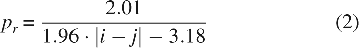 |
obtained from fitting the probability obtained from a Monte Carlo simulation (note that the ideal-chain approximation would have been too poor, due to the small values of |i − j| in which we are interested).
The observation of a contact between residues i and j in m simulations over a total of n can be associated either to the hypothesis that the contact is formed because of an accidental event or to the hypothesis that it is due to a specific mechanism. The probability that a specific mechanism is taking place given the observation of a contact in m simulations over a total of n can be calculated by the Bayes' theorem, that is
 |
The conditional probability that a contact is specific if it is observed to be formed in three simulations over three (i.e., m = n = 3) using Equation 2 is displayed in Figure 8. The probability pr that a contact with | i − j| > 5 is formed by accident is small enough that if one observes it always forming in three independent simulations, the probability that it is not formed by accident is essentially one. If one wants to save time and perform only one simulation, the certainty about the specificity of the formation of a given contact (m = 1, n = 1) holds only if the two residues are separated by ∼20 other residues. If one performs three independent simulations and observes the formation of the contact only twice (m = 2, n = 3), some hint about its specificity can be supposed only if it is local (|i − j| < 10), while if it is nonlocal, one can be quite sure that its formation is an accident.
Figure 8.

Likelihood that the formation of contact between residues i and j is not accidental, as a function of their distance | i − j| along the chain if their formation is observed three times over three simulations (curve a), one time over one simulation (curve b), and two times over three simulations (curve c).
Discussion
A set of computationally intensive simulations of four single-domain proteins was performed starting from elongated, structureless conformations. All of them display a collapse to a compact state lacking of any stable secondary structure. The collapse is due to a nonspecific attraction among hydrophobic residues.
The direct comparison of the present results with experimental data is not straightforward, because it is not granted that the stationary state we observe in the simulations for each protein corresponds to the denatured state. Even if that is the case, as suggested by the stationary character of the macroscopic quantities recorded in the simulations, there is no evidence that the protein explores the full conformation phase space so as to guarantee that any macroscopic quantity associated with the protein is stationary. As a consequence, one needs to carefully check the time dependence of any quantity we compare with experiments. If stably structured regions are found in multiple (short) simulations, it is sensible to expect they would also be structured in the denatured state under native (biological) conditions.
The denatured state of a number of proteins has been characterized experimentally. The extrapolation to zero guanidine concentration of the Rg of protein L, calculated by FRET (Sherman and Haran 2006), is 1.7 nm, corresponding to a globular state, although slightly larger than that obtained by the simulations (Rg = 1.3 nm). A SH3 domain whose denatured state has been characterized under native conditions is that of the drk protein (Mok et al. 1999). This is a domain structurally similar to the src-SH3, but unstable in water at room temperature. The conformations compatible with the NOE signals display an Rg of 1.1 nm, corresponding to a remarkably compact denatured state and in agreement with the result or simulations (Rg = 1.3 nm). On the other hand, the denatured state of CI2 has been described as a random coil (Kazmirski et al. 2001) on the basis of secondary chemical shifts in 6.4 M guanidine chloride and of a MD simulation performed at 498K and lasting for 20 ns. These results are not very informative about the features displayed by the denatured state of CI2 under native conditions because guanidine chloride increases consistently the gyration radius of proteins (Sherman and Haran 2006), and the simulation is done at a temperature that is much higher than that of biological relevance and for a timescale too short as compared to that needed for the collapse of CI2 (cf. Fig. 3). Our simulations indicate that the denatured state of CI2 under native conditions is globular, not coiled, although less compact and displaying larger fluctuations than the other three proteins.
The timescale associated with the collapse of the chain seems quite homogeneous for all four proteins studied and is of the order of tens of nanoseconds. As a rough comparison, the kinetics of the hydrophobic collapse of BBL (a protein of length comparable to those studied above), studied by FRET, starting from the acid-denatured state of the protein, takes place in ∼60 ns (Sadqui et al. 2003). This finding is compatible with the results of the simulations discussed above. The data indicate the collapse of BBL is faster than secondary structure formation, a result also found in the simulations of all four proteins studied.
These simulations we have carried out highlight the formation of a small number of stable contacts on the same timescale of the chain collapse, but not as a trivial consequence of it. These contacts are mainly local and, interestingly, native. Among these we find, in the case of src-SH3, those associated with the n-src loop and the 310-helix loop. Standard interpretation of φ-value analysis indicates these regions are not formed in the transition state (Riddle et al. 1999). However, the same analysis highlights that in the 310-helix, mutations have no effect on stability and that the n-src loop is the region of SH3 where most mutations cause unusual kinetic consequences, that is either increase or decrease both folding and unfolding rates, leading again to ΔΔGDN ≈ 0. The formation of these contacts in the denatured state is not incompatible with the absence of destabilization upon mutations in these regions.
Protein G and protein L display the asymmetric behavior that characterizes also the transition state, where the former populates the second hairpin (McAllister et al. 2000) while the latter populates the first hairpin (Kim et al. 1998). NMR experiments also show a nonrandom behavior in the first hairpin of protein L in 2 M guanidinium chloride (Yi et al. 2000). Our simulations indicate that the turn of the second hairpin of protein G (turn 4) is already formed in the denatured state, together with few loops of the helix (contacts 24–27) as well as native contacts between the C and the α-helix and the third turn, while the first hairpin displays two nonnative interactions (7–10, 17–20) and two (also nonnative) contacts with the α-helix. Protein L populates in the denatured state mainly the loop defined by the first hairpin, and few contacts (both native and nonnative) in the second one. In agreement with the results of multiple mutations (Kim et al. 1998), the helix is completely disrupted.
Our results on protein G and src-SH3 can also be compared with the simulations by Brooks and coworkers (Sheinerman and Brooks 1998a,b, Shea et al. 2002). Here, the free-energy surface is sampled by means of short molecular dynamics simulations starting from a set of characteristic conformations extracted from high-temperature unfolding trajectories. It is observed that in the regions of the free-energy characterized by compact unfolded conformations, only a small set of native contacts is stable. In the case of protein G, these contacts are localized in both in the N-terminal and in the center of the α-helix (regions 24–26 and 29–33), in good agreement with our results. In the case of src-SH3, the contacts are in the RT loop and in the fifth β-strand, while we see early contacts in the src-loop and between the 310-helix and the fifth β-strand.
A comparison can also be made between the present results and the zipping model (Ozkan et al. 2007), which allows us to identify the nucleation regions of the protein based on the kinetics of its constituting fragments. In the case of protein G, the nucleation regions result to be the segments 6–15, which then grows, stabilizing the whole first hairpin, and 45–52, which grows, stabilizing the second hairpin and the second half the helix. In agreement with the idea at the basis of the zipping model, we observe in the first nanoseconds only the formation of local contacts: Two native contacts belong to the region 45–52, and one nonnative contact in the region 6–15. Differently from the work of Ozkan and coworkers, we oberve stable contacts scattered in other regions of protein G (cf. Table 2). The main difference between the two models relies on the fact that we simulate the whole protein, while the zipping model simulates its fragments separately. Consequently, one can make the hypothesis that some correlations between residues that belong to the different fragments used in the zipping model contribute to the stabilization of these contacts.
The case of CI2 is particularly interesting because it is the prototype of the “nucleation-condensation” folding model (Karplus and Weaver 1976), according to which a local native structure is stabilized before the overall formation of the native tertiary structure of the protein. Our simulations show that there are stable native contacts also in the denatured state of CI2, involving the loop at the C end of the helix and the loop at the end of the β4 strand. Simulations show that these native contacts are also preserved in guanidinium chloride. Under these conditions the protein does not display any hydrophobic collapse, supporting the idea that the formation of these (local) contacts is independent of the collapse of the chain and that they are particularly stable. This result is important from an experimental point of view. In fact, it suggests that the degree of local structure that is observed in the protein denatured by chemical agents is similar to that present in the denatured state under native conditions, which is the state relevant for determining the folding properties.
Although CD experiments on CI2 do not detect any secondary structure in the denatured state, NMR experiments in 6.4 M guanidine chloride report secondary chemical shifts compatible with native structure in the C end of the helix region (Kazmirski et al. 2001). In terms of residual structure, CI2 seems not qualitatively different from the other three proteins studied. That is, the observed residual structure does not correspond to any particular secondary structure.
Our results on CI2 can also be compared with the high-temperature unfolding simulations by Daggett and coworkers (Kazmirski et al. 2001; De Jong et al. 2002). In these works it is shown that the high-temperature conformations beyond the transition state do not display any native structure except in the α-helix and that the protein explores conformations with a very high value of Rg (>2 nm). Quenching the temperature to native-like conditions cause the hydrophobic collapse of these structures and the formation of some native interaction, in particular between the helix and the third β-sheet, in accordance with the results of our simulations.
Within this context, it proves useful to compare the results of the all-atom, explicit solvent molecular dynamics simulations discussed above with those obtained with the help of a perfect funneled model (only native contacts allowed) that makes use of a weighted Go contact potential (Sutto et al. 2006) and allows for an exhaustive search in conformational space.
In the case of the SH3 domain these calculations show that the contacts formed early are those within the n-src loops and between the 310-helix and β5-sheet, as observed in the present calculations (see Table 2). The similarities between all-atom and Go-model results become even more striking if one uses as criteria for native local structures the native position of a residue in two of the three trajectories. In this case one finds, aside from the structures mentioned above, also those corresponding to β1- and β2-sheets.
In the case of protein G, the perfectly funneled model shows early contacts within the second β-hairpin (46–49, 48–51) and within the α-helix (23–26), as well between β2 and α-helix (20–23) and between turn 3 and α-helix (35–39) that essentially agree with the present results (cf. Table 2). In the case of CI2, Go–model results indicate the early formation of the turns between the α-helix and β3 (22–25) as well between the fourth and the fifth β-strands (50–57), in overall agreement with the present results (cf. Table 2).
The Go-model results have been interpreted (Sutto et al. 2006) in terms of a hierarchical folding scenario, where few local elementary structures (LES) are formed in the initial stage of the folding process and eventually dock together to drive the protein into the native free-energy basin (Broglia et al. 2004). The present simulations suggest that some of such LES (or, anyway, part of them) are already formed in the first 50 ns in the proteins analyzed.
Concluding, all-atom molecular dynamics simulations in explicit solvent are suitable for studying the very first events in protein folding. These events include the hydrophobic collapse and the formation of specific native contacts that, as a rule, belong to regions of the protein that eventually form the folding nucleus, docking together in the transition state. The formation of native contacts between residues that are close along the chain helps the protein to display short structured segments already in the denatured state. These are likely to play an important role in the folding dynamics of the protein, helping to solve Levinthal's paradox.
Materials and Methods
Three molecular dynamics runs of 50 ns each, starting from three different extended structures, were carried out for each protein. The starting structures are generated from crystallographic protein (codes 1FMK, 1PGB, 2PTL, and 2CI2) making use of the PyMOL sculpting tool (DeLano Scientific). The Ramachandran dihedrals are increased to values close to 180° in order to have a backbone that is elongated, in order not to display any degree of structure, and bent, in order to keep the proteins in a small volume. If prolines were present in the sequence their native isomerization was conserved. Molecular dynamics simulations are performed with the Gromacs molecular dynamics package (Berendsen et al. 1995; Lindahl et al. 2001; Van Der Spoel et al. 2005). The interactions were described using the GROMOS 53A6 force field (Oostenbrink et al. 2004, 2005), and virtual-site atoms for hydrogens were used to speed up the simulation (Miyamoto and Kollman 1992; Hess et al. 1997), allowing the time step for the molecular dynamic integration to be as high as 0.004 ps. The system was enclosed in a dodecahedron box with periodic boundary conditions and solvated with SPCE water molecules (Berendsen et al. 1987). The system charge was neutralized, adding the proper number of positive (Na+) or negative (Cl−) ions. Van der Waals interactions were cut off at 1.4 nm, and the long-range electrostatic interactions were calculated by the particle mesh Ewald algorithm (Essman et al. 1995), with a mesh space of at least 0.130 nm. The list of neighbors was updated every five steps (0.020 ps). The system is coupled with a Nosé–Hoover thermal bath (Nosé 1984; Hoover 1985). The model to describe guanidinium chloride used in the calculations (CI2 in 3.9 M of the denaturant) is that developed by Camilloni et al. (2008). The reference correlation function is calculated for each protein performing Monte Carlo simulations of an homopolymer, modeled as a chain of C α of the same length, tied together by rigid bonds of a length of 0.38 nm. The interaction energy between two C α is −1 if they are closer than 0.75 nm and separated along the chain by at least other two C α. A hardcore of radius 0.4 nm prevents their overlap. The temperature is chosen in such a way that the average gyration radius of the model is equal to that of the all-atom simulation.
Electronic supplemental material
In the Supplemental material we replot Figures 4–7 in color, and we show the figures displaying the RMSD and Rg for all the trajectories, the relative secondary structure data, and the contact distance maps. Moreover, there is a table in which the contact found in two out of three simulations, not correlated with the collapse, are listed.
Acknowledgments
The authors acknowledge the financial support of the 2003 FIRB program of the Italian Ministry of Scientific Research and of INFN. Computational resources of CILEA have made this work possible.
Footnotes
Supplemental material: see www.proteinscience.org
Reprint requests to: Guido Tiana, Department of Physics, University of Milano, via Celoria, 16, 20133 Milano, Italy; e-mail: guido.tiana@mi.infn.it; fax: 39-02-50317487.
Article and publication are at http://www.proteinscience.org/cgi/doi/10.1110/ps.035105.108.
References
- Berendsen, H.J.C., Grigera, J.R., Straatsma, T.P. The missing term in effective pair potentials. J. Phys. Chem. 1987;91:6269–6271. [Google Scholar]
- Berendsen, H.J.C., van derSpoel, D., vanDrunen, R. Gromacs: A message–passing parallel molecular dynamics implementation. Comput. Phys. Commun. 1995;91:43–55. [Google Scholar]
- Broglia, R.A., Tiana, G. Hierarchy of events in the folding of model proteins. J. Chem. Phys. 2001;114:7267–7272. [Google Scholar]
- Broglia, R.A., Tiana, G., Provasi, D. Simple model of protein folding and of non-conventional drug design. J. Phys. Cond. Mat. R. 2004;16:111–144. [Google Scholar]
- Broglia, R.A., Tiana, G., Sutto, L., Provasi, D., Simona, F. The physics of protein folding and of non-conventional drug design: Attacking aids with its own weapon. Rivista del Nuovo Cimento. 2006;29:1–119. [Google Scholar]
- Camilloni, C., Guerini Rocco, A., Eberini, I., Gianazza, E., Broglia, R.A., Tiana, G. Urea and guanidinium chloride denature protein l in different ways in molecular dynamics simulations. Biophys. J. 2008;94:4654–4661. doi: 10.1529/biophysj.107.125799. [DOI] [PMC free article] [PubMed] [Google Scholar]
- De Jong, D., Riley, R., Alonso, D.O.V., Daggett, V. Probing the energy landscape of protein folding/unfolding transition states. J. Mol. Biol. 2002;319:229–242. doi: 10.1016/S0022-2836(02)00212-7. [DOI] [PubMed] [Google Scholar]
- Duan, Y., Kollman, P.A. Pathways to a protein folding intermediate observed in a 1-microsecond simulation in aqueous solution. Science. 1998;282:740–744. doi: 10.1126/science.282.5389.740. [DOI] [PubMed] [Google Scholar]
- Essman, U., Perela, L., Berkovitz, M.L., Darden, T., Lee, H., Pedersen, L.G. A smooth particle mesh ewald method. J. Chem. Phys. 1995;103:8577–8592. [Google Scholar]
- Ferguson, N., Fersht, A.R. Early events in protein folding. Curr. Opin. Struct. Biol. 2003;13:75–81. doi: 10.1016/s0959-440x(02)00009-x. [DOI] [PubMed] [Google Scholar]
- Fersht, A. Structure and mechanism in protein science. Freeman; New York: 1999. [Google Scholar]
- Hess, B., Bekker, H., Berendsen, H.J.C. Lincs: A linear constraint solver for molecular simulations. J. Comput. Chem. 1997;18:1463–1472. [Google Scholar]
- Hoover, W.G. Canonical dynamics: Equilibrium phase-space distributions. Phys. Rev. A. 1985;31:1695–1697. doi: 10.1103/physreva.31.1695. [DOI] [PubMed] [Google Scholar]
- Karplus, M., Weaver, D.L. Protein folding dynamics. Nature. 1976;260:404–406. doi: 10.1038/260404a0. [DOI] [PubMed] [Google Scholar]
- Kazmirski, S.L., Wong, K.B., Freund, S.M.V., Tan, Y.J., Fersht, A.R., Daggett, V. Protein folding from a highly disordered denatured state: Folding pathway of chymotrypsin inhibitor 2 at atomic resolution. Proc. Natl. Acad. Sci. 2001;98:4349–4354. doi: 10.1073/pnas.071054398. [DOI] [PMC free article] [PubMed] [Google Scholar]
- Kim, D.E., Yi, Q., Gladwin, S.T., Goldberg, J.M., Baker, D. The single helix in protein l is largely disrupted at the rate–limiting step in folding. J. Mol. Biol. 1998;284:807–815. doi: 10.1006/jmbi.1998.2200. [DOI] [PubMed] [Google Scholar]
- Lindahl, E., Hess, B., van derSpoel, D. Gromacs 3.0: A package for molecular simulation and trajectory analysis. J. Mol. Model. 2001;7:306–317. [Google Scholar]
- McAllister, E.L., Alm, E., Baker, D. Critical role of β-hairpin formation in protein g folding. Nat. Struct. Biol. 2000;7:669–763. doi: 10.1038/77971. [DOI] [PubMed] [Google Scholar]
- Miyamoto, S., Kollman, P. Settle: An analytical version of the shake and rattle algorithms for rigid water models. J. Comput. Chem. 1992;13:952–962. [Google Scholar]
- Mok, Y.K., Kay, C.M., Kay, L.E., Forman-Key, J. NOE data demonstrating a compact unfolded state for an sh3 domain under non-denaturing conditions. J. Mol. Biol. 1999;289:619–638. doi: 10.1006/jmbi.1999.2769. [DOI] [PubMed] [Google Scholar]
- Navon, A., Ittah, V., Laity, J.H., Scheraga, H.A., Haas, E., Gussakovsky, E.E. Local and long-range interactions in termal unfolding transition state of bovine pancreatic ribonuclease a. Biochemistry. 2001;40:93–104. doi: 10.1021/bi001945w. [DOI] [PubMed] [Google Scholar]
- Nosé, S. A molecular dynamics method for simulations in the canonical ensemble. Mol. Phys. 1984;52:255–268. [Google Scholar]
- Oostenbrink, C., Villa, A., Mark, A.E., van Gunsteren, W.F. A biomolecular force field based on the free enthalpy of hydration and solvation: The gromos force-field parameter sets 53a5 and 53a6. J. Comput. Chem. 2004;25:1656–1676. doi: 10.1002/jcc.20090. [DOI] [PubMed] [Google Scholar]
- Oostenbrink, C., Soares, T.A., van der Vegt, N.F., van Gunsteren, W.F. Validation of the 53a6 gromos force field. Eur. Biophys. J. 2005;34:273–284. doi: 10.1007/s00249-004-0448-6. [DOI] [PubMed] [Google Scholar]
- Ozkan, S.B., Wu, G.A., Chodera, J.D., Dill, K.A. Protein folding by zipping and assembly. Proc. Natl. Acad. Sci. 2007;104:11987–11992. doi: 10.1073/pnas.0703700104. [DOI] [PMC free article] [PubMed] [Google Scholar]
- Riddle, D., Grantcharova, V., Santiago, J., Alm, E., Ruczinski, I., Baker, D. Experiment and theory highlight role of native state topology in sh3 folding. Nat. Struct. Biol. 1999;6:1016–1024. doi: 10.1038/14901. [DOI] [PubMed] [Google Scholar]
- Sadqui, M., Lapidus, L., Muñoz, V. How fast is protein hydrophobic collapse? Proc. Natl. Acad. Sci. 2003;100:12117–12122. doi: 10.1073/pnas.2033863100. [DOI] [PMC free article] [PubMed] [Google Scholar]
- Shea, J.-E., Onuchic, J.N., Brooks, C.L. Probing the folding free energy landscape of the src-sh3 protein domain. Proc. Natl. Acad. Sci. 2002;99:16064–16068. doi: 10.1073/pnas.242293099. [DOI] [PMC free article] [PubMed] [Google Scholar]
- Sheinerman, C., Brooks, C.L. Calculations on folding of segment b1 of streptococcal protein g. J. Mol. Biol. 1998a;278:439–456. doi: 10.1006/jmbi.1998.1688. [DOI] [PubMed] [Google Scholar]
- Sheinerman, C., Brooks, C.L. Molecular picture of folding of a small α/β protein. Proc. Natl. Acad. Sci. 1998b;96:1562–1567. doi: 10.1073/pnas.95.4.1562. [DOI] [PMC free article] [PubMed] [Google Scholar]
- Sherman, E., Haran, G. Coil-gobule transition in the denatured state of a small protein. Proc. Natl. Acad. Sci. 2006;103:11539–11543. doi: 10.1073/pnas.0601395103. [DOI] [PMC free article] [PubMed] [Google Scholar]
- Shirts, M., Pande, V.S. Computing: Screen savers of the world unite! Science. 2000;290:1903–1904. doi: 10.1126/science.290.5498.1903. [DOI] [PubMed] [Google Scholar]
- Shortle, D. The denatured state (the other half of the folding equation) and its role in protein stability. FASEB J. 1996;10:27–34. doi: 10.1096/fasebj.10.1.8566543. [DOI] [PubMed] [Google Scholar]
- Sutto, L., Tiana, G., Broglia, R.A. Sequence of events in folding mechanism: beyond the go model. Protein Sci. 2006;15:1638–1652. doi: 10.1110/ps.052056006. [DOI] [PMC free article] [PubMed] [Google Scholar]
- Van Der Spoel, D., Lindahl, E., Hess, B., Groenhof, G., Mark, A.E., Berendsen, H.J.C. Gromacs: Fast, flexible, and free. J. Comput. Chem. 2005;26:1701–1718. doi: 10.1002/jcc.20291. [DOI] [PubMed] [Google Scholar]
- Yi, Q., Scalley-Kim, M.L., Alm, E., Bajer, D. Nmr characterization of residual structure in the denatured state of protein l. J. Mol. Biol. 2000;299:1341–1351. doi: 10.1006/jmbi.2000.3816. [DOI] [PubMed] [Google Scholar]