α-Synuclein Tertiary Contact Dynamics

Abstract

Tertiary contact formation rates in α-synuclein, an intrinsically disordered polypeptide implicated in Parkinson's disease, have been determined from measurements of diffusion-limited electron transfer kinetics between triplet excited tryptophan:3-nitrotyrosine pairs separated by 10, 12, 55, and 90 residues. Calculations based on a Markovian lattice model developed to describe intrachain diffusion dynamics for a disordered polypeptide give contact quenching rates for various loop sizes ranging from 6 to 48 that are in reasonable agreement with experimentally determined values for small loops (10−20 residues). Contrary to expectations, measured contact rates in α-synuclein do not continue to decrease as the loop size increases (≥35 residues), and substantial deviations from calculated rates are found for the pairs W4-Y94, Y39-W94, and W4-Y136. The contact rates for these large loops indicate much shorter average donor-acceptor separations than expected for a random polymer.

INTRODUCTION

Proteins can adopt a continuum of structures ranging from tightly folded to highly extended with conformational dynamics spanning timescales from picoseconds to seconds.¹ The dynamics of intrachain-contact formation in disordered polypeptides can provide insights into the stiffness of the polymer and the range of structures present in the protein ensemble.^2,3 Moreover, the formation of tertiary contacts is a necessary step in the formation of folded structures.^4-6 Much previous experimental^4-13 and theoretical^14-17 work has focused on determining tertiary contact rates in order to set a folding speed limit.

α-Synuclein (α-syn), a protein implicated in Parkinson's disease,^18,19 does not fold in aqueous solution, and spectroscopic studies suggest that the polypeptide is extended and conformationally flexible.^20-22 The rates of tertiary contact formation in α-syn^2,23 are of particular interest, because large amplitude motions of the polypeptide chain could play a critical role in the aggregation process that is believed to lead to Parkinson's disease.^24,25 Using photoinduced electron transfer (ET) from triplet-excited tryptophan (³W*) to 3-nitrotyrosine (Y(NO₂)), we determined the timescales for contact formation in donor(D)-acceptor(A)-containing α-synucleins (loop sizes, n, separating D and A of 15, 20, 35, 42, and 132 residues) that revealed differences in chain stiffness and nonrandom structural preferences in distinct regions of the protein.^2,26 We also simultaneously analyzed the fluorescence energy transfer and ET kinetics² to define equilibrium distributions of donor-acceptor distances (P(r)) as well as diffusion coefficients.

To map α-syn conformational dynamics in other distinct polypeptide regions, we have extended our work to include four DA pairs with smaller (10 and 12) and intermediate (55 and 90) loop lengths. Of special interest are the intermediate loops: one (Y39-W94) falls in the NAC (non-amyloid β component, Glu61-Val95) region, which is a possible nucleation site for protein aggregation (Figure 1);^27-30 and the other loop contains D and A residues (W4-Y94) that have been shown by analysis of NMR spectroscopic data to be in close proximity in the micelle-bound structure.³¹ In order to evaluate the experimental contact formation rates, we have formulated a lattice model for loop formation in random polymers that explicitly accounts for geometrical exclusion effects. To implement such a model, the dimensionality (d) and coordination (ν) of the (reaction) space accessible to the diffusing donor must be specified. The intrachain-diffusion-reaction event can then be studied by implementing the theory of finite Markov processes,^32,33 and the dynamics quantified by solving numerically the associated stochastic master equation. In the language of Markov chain theory, the donor is regarded as undergoing a “random walk” in the vicinity of a “deep trap” (i.e., the acceptor) and the time elapsed before the “walker” is trapped (i.e., reacts) can be calculated.

Figure 1.

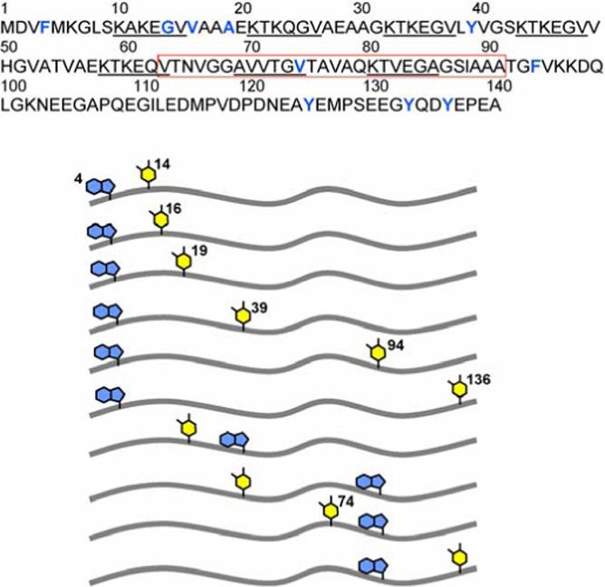
(upper) Primary amino-acid sequence of human α-syn. The NAC (non-amyloid β component) region is boxed in red. Residues highlighted in blue either have been mutated (W, F, Y) or chemically modified (Y(NO₂)). (lower) Schematic representations of the ten different α-syn variants and the locations of D(Trp, violet)-A(Y(NO₂), yellow) pairs used in this study.

MATERIALS AND METHODS

Protein Preparation, Modification, and Characterization

The wild-type human α-syn expression plasmid (pRK172) was provided by M. Goedert (Medical Council Research Laboratory of Molecular Biology, Cambridge, U.K.).³⁴ Single Trp residues were introduced at two different aromatic-residue positions (F4, F94) and single Tyr residues were introduced at positions 14, 16, and 94 by site-directed mutagenesis. Four different W-Y pair-containing synucleins were prepared: W4-Y14, W4-Y16, Y39-W94, and W4-Y94 with loop sizes of 10, 12, 55, and 90. The proteins also had all four native Tyr residues mutated to Phe residues (Y39F/Y125F/Y133F/Y136F) except for the Y39-W94 protein. All site-directed mutagenesis reactions were performed using a QuickChange kit (Stratagene). All mutations were confirmed by DNA sequencing (Caltech DNA Sequencing Core Facility).

Recombinant α-syn proteins were expressed and purified according to published procedures.²⁶ Briefly, after cell lysis crude protein extract was chromatographed on a Q-Sepharose Fast Flow column (GE Healthcare) equilibrated with 20 mM Tris buffer (pH 8.0) and eluted with a linear NaCl gradient (0−500 mM). Fractions containing α-syn were pooled (YM3 membranes, Millipore) and further purified on a Mono-Q column (GE Healthcare). To prepare the nitrated proteins, tetranitromethane in ethanol [1% (vol/vol), 75 μL] was added dropwise to a stirred deoxygenated protein solution (70−100 μM in 20 mM Tris buffer with 200−300 mM NaCl at pH 8.0, 850 μL) in the dark. After 10 min, a second aliquot of tetranitromethane was added. The reaction was terminated by gel filtration chromatography with a HiPrep Desalting column (GE Healthcare) and finally the labeled protein was purified on a Mono Q column.

Time-Resolved Absorption Measurements

³W* decay kinetics were measured as previously described with some modifications.² All protein samples (7−25 μM in 20 mM NaPi, pH 7.4) were deoxygenated by repeated evacuation/Ar fill cycles on a Schlenk line. N₂O was used as a solvated-electron scavenger. The second harmonic (290 nm) of a nanosecond Nd:YAG pumped optical parametric oscillator laser (Spectra-Physics) and an Ar-ion laser (457.9 nm) were used as the excitation source and probe light, respectively. The probe laser was passed through the sample multiple times increasing the path length from 1- to 11-cm, thereby improving the sensitivity of our measurement by nearly an order of magnitude. In addition, the pump beam was double passed transversely through the probe volume (Supporting Information). Transient absorption kinetics were detected by a photodiode and recorded using an 8-bit, 500-MHz digital oscilloscope (LeCroy 9354A). All protein samples were filtered through Microcon YM-100 (MWCO 100kD) (Millipore) spin filter units to remove oligomeric material prior to measurements.

Data Analysis

Measured kinetics traces were converted to absorbance changes [−log₁₀(I_sample/I_reference)], logarithmically compressed (100 points per time decade), and normalized [OD(t)−OD(t_∞)/OD(t₀)−OD(t_∞)]. We have used two algorithms to invert our kinetics data [I(t)=Σ_kP(k)exp(−kt)] with regularization methods that impose additional constraints on the properties of P(k). We have fit the kinetics data using a MATLAB (The Math Works, Inc.) algorithm (LSQNONNEG; hereafter referred to as NNLS) that minimizes the sum of the squared deviations (χ²) between observed and calculated values of I(t), subject to a nonnegativity constraint on P(k). NNLS fitting produces the narrowest P(k) distributions. Information theory suggests that the least biased solution to this inversion problem minimizes χ² and maximizes the breadth of P(k).³⁵ This regularization condition can be met by maximizing the Shannon-Jaynes entropy of the rate-constant distribution [S=−Σ_kP(k)ln(P(k))], implicitly requiring that P(k) ≥ 0 (∀k).³⁶ The balance between χ² minimization and entropy maximization was determined by graphical L-curve analysis.³⁷ This approach yields upper limits for the widths of P(k) consistent with our experimental data. The P(k) distributions from maximum-entropy (ME) fitting were broader than those obtained with NNLS fitting, but exhibited comparable maxima. Average contact rate constants were estimated using the following relation: <k>⁻¹ ≡ {Σ P(k)/k}/{Σ P(k)}. Uncertainties in these quantities were estimated using a Monte Carlo sampling method.³⁸ The results from NNLS and ME fitting are given in the Supporting Information.

Lattice Model

Consider a polypeptide chain with a donor (D) and acceptor (A) separated by 12 residues (Figure 2). To visualize tertiary contact formation, suppose first that the motion of the chain is restricted to two dimensions (d=2); then, in the dynamic motion of the polypeptide chain, a D-A pair (each residue of length L) can be brought into contact if the chain forms a planar loop (of area A=3 L² cot 15). In d=3, the loop need not be planar; to account for this, in what follows we shall consider the volume (in fact, the maximum volume) enclosed by a loop of length n.

Figure 2.

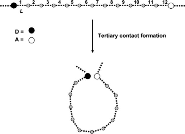
Schematic representation of tertiary contact formation in a polypeptide chain with a donor (D) and acceptor (A) separated by 12 residues with each residue of length L.

To account for excluded volume effects, we proceed by formulating a lattice (rather than continuum) model, and identify the (maximum) lattice volume encompassed by a given setting of n. Considering first a simple cubic lattice (dimension, d=3; coordination, ν=6), if the position of the acceptor is anchored at a vertex site of the lattice, then the maximum volume encompassed by a n=12 loop includes all sites on or within a 3×3×3 simple cubic lattice of 27 sites. We specify that all down-range segments of the polypeptide chain are excluded from this volume. Further, since we are primarily interested in tracking donor displacements in the near neighborhood of the acceptor, donor excursions to sites external to the defining volume will be neglected.

As the polypeptide chain undergoes positional fluctuations, the donor will visit (eventually) all lattice sites in the defining volume. Although these donor displacements are totally random, we can calculate (via Markov theory) the average number of displacements before an irreversible electron transfer reaction occurs between donor and acceptor (i.e., before the “walker” is “trapped”). Assuming that each displacement of the donor takes place in one time step, then the mean number of displacements (or mean walklength <x>) gauges the mean reaction time.

A more detailed description of the dynamics of the system can be obtained by solving the associated stochastic master equation,^32,33 determining the full eigenvalue spectrum and associating the smallest eigenvalue(s) with the rate constant(s) characterizing the diffusion-controlled reactive event. Again, from Markov theory, as the system size increases, the reciprocal of the mean walklength <x> approaches asymptotically the magnitude of the smallest eigenvalue of the associated master equation, a fact that can be used to gauge the internal consistency of the numerical calculations. The mean walklengths and eigenvalues reported in this study are the numerically exact values, i.e., once the model is defined, no further approximations are made in calculating these values.³³

The above discussion was predicated on the assumption that the site-to-site coordination available to the segments of a polypeptide chain could be represented by a d = 3 simple cubic lattice. To account for excluded-volume effects within the context of a geometry more representative of the actual coordination of a polypeptide chain, we consider a family of d = 3 tetrahedral lattices of coordination ν = 4, and repeat the calculations above for simple cubic lattices. Here again, the acceptor is pinned at one of the vertex sites, and the dynamics studied as a function of loop size.

To summarize, as a consequence of the spatial and temporal fluctuations of a polypeptide chain in its ambient environment, a donor separated by n residues from an acceptor will undergo random displacements subject to the excluded volume and geometric constraints noted above. The underlying stochastic process can be characterized by calculating the evolution of two signatures of the system. The first is the mean number <x> of displacements of the donor before the loop closes and an irreversible electron transfer reaction takes place. Secondly, the full eigenvalue spectrum can be calculated, recognizing that the smallest eigenvalue can (usually) be placed in correspondence with the experimentally determined rate constant. If there are two (or more) “small” eigenvalues that are similar in magnitude, then the decay will not be strictly exponential, but the evolution of the system in the long-time limit will still be dominated by the smallest eigenvalue. The smallest eigenvalue and average walklength <x> are listed for a series of n values for simple cubic lattices in Table 1 and for tetrahedral lattices in Table 2.

Table 1.

Rate constants as a function of loop size n: Simple cubic lattices.

loop (n)	lattice	sites (N)	mean displacement (<x>)	minimum eigenvalue	error (%)a
6	2×2×2	8	16.571	0.059041	2.21
8	2×2×3	12	29.376	0.032785	3.83
10	3×3×2	18	47.130	0.020701	2.50
12	3×3×3	27	72.274	0.013630	1.51
14	3×3×4	36	102.855	0.009559	1.71
18	4×4×4	64	194.586	0.005084	1.10
24	5×5×5	125	409.609	0.002422	0.80
30	6×6×6	216	743.332	0.001337	0.62
36	7×7×7	343	1221.708	0.000814665	0.47

^a% Error=(1/<x> — λ(min))/λ(min)×100.

Table 2.

Rate constants as a function of loop size n: Tetrahedral lattices.

loop (n)	lattice sites (N)	mean displacement (<x>)	minimum eigenvalue	Errora (%)
	5	19	0.052178	0.87
6	14	77.153	0.012881	0.62
12	30	195.724	0.005038	1.41
18	55	398.954	0.002477	1.19
24	91	703.504	0.001408	0.96
48	285	2505.447	0.0003991	0.033

^a% Error=(1/<x> — λ(min))/λ(min)×100.

RESULTS AND DISCUSSION

We have measured ³W*/Y(NO₂) ET rates in ten different α-syn mutants. Fits of the kinetics data employing constrained least squares (NNLS) and maximum entropy (ME) methods (Table 3 and supporting information) are consistent with k_contact values from our earlier work (biexponential fits).² Intrachain contact times in a polymer should depend on the average distance between the contact points and the stiffness of the intervening chain. If α-syn were a random polymer, then ³W*/Y(NO₂) ET rates would decrease monotonically with increasing loop size. We find that the contact rates for loop sizes between 10 and 132 residues fall in a range between 10⁵ and 10⁷ s⁻¹ (Table 3, Figure 3). The observed rates, however, do not exhibit a monotonic correlation with loop size. For n ≤ 20, contact rates decrease with increasing loop size, but level off in the range of 1−5 × 10⁵ s⁻¹ for larger loops. Although the uncertainties in average rate constants are large in some cases, our data clearly demonstrate that contact rates do not simply continue to decrease with increasing loop size.¹⁶ The leveling of contact rates for n > 20 suggests that the average distance between ³W* and Y(NO₂) is not increasing for these larger loops.

Table 3.

Contact quenching rates for Trp-and-Tyr(NO₂)-containing α-synucleins

loop (n)	W site	Y(NO2) site	<k> (s−1)a
10	4	14	5.1 × 106
12	4	16	2.3 × 106
15b	4	19	7.2 × 105
20b	19	39	2.6 × 105
20b	94	74	2.8 × 105
35b	4	39	5.3 × 105
42b	94	136	2.3 × 105
55	94	39	1.6 × 105
90	4	94	2.2 × 105
132b	4	136	3.9 × 105

^aaverage rate constants (<k>) were extracted from NNLS distributions according to the following: <k>⁻¹ ≡ {Σ P(k)/k}/{Σ P(k)}.

^bRef. ².

Figure 3.

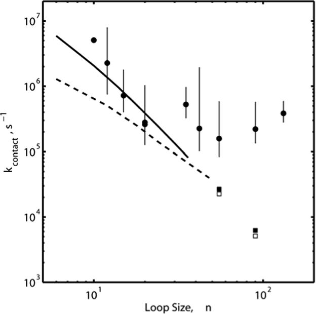
Contact rate constants calculated as functions of loop size (n) for simple cubic (solid line) and tetrahedral (dashed lines) lattices. Rates calculated using the trace relationship for n=55 and n=90 for simple cubic (open squares) and tetrahedral (filled squares) lattices. The filled circles represent average contact rate constants measured by Y(NO₂) quenching of ³W* in α-synuclein (20 mM NaPi, pH 7.4, 22 °C, Table 3).²

NMR studies have provided insights into the ensembles of α-syn structures present in aqueous solution. Contact maps derived from paramagnetic relaxation enhancement measurements suggest that the D-A pairs used in our studies of large loops (n > 20) are in regions of the protein in which contact probabilities are substantially greater than expected for a random polymer.²¹ Residual dipolar coupling measurements in weakly aligned α-syn have been interpreted in terms of five distinct protein domains.³⁹ Our D-A pairs are distributed throughout these domains and the contact dynamics indicate that they are highly fluxional structures.

It has been proposed from NMR experiments in the presence of SDS micelles that α-syn rearranges into two anti-parallel helices (N-terminal from residues 3−37, and C-terminal from residues 45−92, hence, bringing together the N- and C-termini).³¹ The calculated distance from Phe4 to Phe94 in the wild-type protein is ∼24 Å based on this model (using PDB accession number 1XQ8). If α-syn retains residual structure reminiscent of this detergent-associated conformation in solution, then the contact quenching rates would deviate from those expected for a random polymer. It also is plausible that the diffusion coefficients vary among labeling sites because of differences in chain stiffness throughout the polypeptide.

We have developed a three-dimensional Markovian lattice model to compare the experimental α-syn contact rates with those expected for a random polymer. If we scale the theoretically computed rate constants in Tables 1 and 2 by a factor of 10⁸, the results can be placed in correspondence with our experimental results.² Both data sets are plotted in Figure 3; interestingly, the results are in qualitative agreement with the experimental data for n ≤ 20, but the substantial deviations from theoretical predictions for larger loops indicate that there are nonrandom structures in these regions. The rates for W4-Y39, W94-Y39, W4-Y94, and Y39-W94 are higher than expected; indeed the average contact rates increase slightly for n = 55, 90, 132. This observation supports our interpretation of the contact rates that the equilibrium distributions of W4-Y94 and W4-Y136 distances include many more compact structures than expected for a random polymer.

The immediate conclusion that can be drawn from comparisons between results obtained for simple cubic lattices versus those for tetrahedral lattices is that the flexibility (or “stiffness”) of the polypeptide chain seems not to have a significant impact on the system dynamics for intermediate and large loop sizes. As may be seen from the data, already in the vicinity of n ∼ 24, the results calculated using the two lattice representations appear to be converging. In fact, in this regime, agreement with the experimental values of the contact quenching rate constant is quite good.

On the other hand, chain flexibility/stiffness, if it is a factor, is likely to become of increasing importance with decreasing loop size. Indeed, in an earlier review, Kiefhaber and coworkers⁸ note that for entropy-controlled intrachain diffusion in freely jointed Gaussian chains, the rate of contact formation should exhibit a power-law dependence on n:

$$k\sim n^{-1.5}$$

They go on to observe that Flory advanced the argument that excluded volume effects should significantly influence the chain dimension.⁴⁰ When they account for excluded volume effects in the end-to-end diffusion model developed by Szabo et al.,¹⁷ they again find a power-law dependence, albeit with a somewhat more negative exponent:⁸

$$k\sim n^{-1.8}$$

If, now, the data in Tables 1 and 2 are fitted (via least squares) to a functional form, k = αn^−a (Figure 3), we determine that:

$$k\sim n^{-2.4}\text{for simple cubic lattices}$$

$$k\sim n^{-1.7}\text{for tetrahedral lattices}$$

Thus, the behavior of the contact-quenching rate constants calculated using a tetrahedral lattice model to account for excluded-volume effects is in line with a result that is consistent with the continuum model developed by Szabo et al.¹⁷

The fact that the simple cubic lattice exhibits a steeper n-dependence of the contact rate constant than the tetrahedral lattice is somewhat unexpected in light of the continuum model results.^8,17 We can rationalize this observation using an expression for the tertiary contact formation rate constant (k_T) developed by Thirumalai:¹⁶

$$k_T=\tau {\left(n\right)}^{-1}=\frac{P\left(n\right)D_0}{\langle r^2\rangle }$$

In this expression, P(n) is the loop-formation probability, D₀ is the effective diffusion coefficient for a single link in the polymer, and 〈r²〉 is the mean-squared distance between the two residues making the contact. In a seminal paper on excluded-volume effects for two- and three-dimensional lattice models, Domb determined for both simple cubic and tetrahedral lattices that 〈r²〉 ∼ n^6/5 in the limit of large n.⁴¹ For values of n ≤ 10, somewhat larger exponents are reported (1.22 − 1.28). We can approximate P(n) by the reciprocal of the number of lattice sites (N); least-squares fitting to a power-law dependence gives P(n) ∼ n^−2.1 for the simple cubic lattice and P(n) ∼ n^−1.4 for the tetrahedral lattice. Combining these results into the Thirumalai expression leads to:

$$k\sim n^{-3.3}\text{for simple cubic lattices}$$

$$k\sim n^{-2.6}\text{for tetrahedral lattices}$$

Although the quantitative agreement between the Markov chain results and contact rates estimated using Thirumalai's expression is only fair, both approaches predict a steeper decrease in contact rate with increasing n for the simple cubic lattice. This behavior is attributable to the faster decrease in loop formation probability with the simple cubic lattice. In other words, the faster growth in configurational entropy as polymer size (n) increases is responsible for a steeper decay in contact rate constants for more flexible polymers.

The data on which the above representations are based (Tables 1 and 2) were limited to loop sizes of small and intermediate lengths. The open question is whether the above behavior persists for very large loop sizes. In particular, although given the systematic decrease in the rate constant as a function of loop size n predicted by the lattice Markovian model (Figure 3), the question is whether this predicted decrease in rate constants persists for very large loops, e.g., n>50. This question can be addressed by taking advantage of a property of the trace of Markovian matrices. In particular, although only the smallest eigenvalues are reported in Tables 1 and 3, the full spectrum of eigenvalues was determined in each case. The eigenvalues calculated are often complex (i.e., having a rational real part and an irrational imaginary part). However, when these eigenvalues are summed, the value of the resultant trace is a ratio of integers (Table 4). Were the lattice subject to periodic boundary conditions, the result would be a simple integer (rather than a ratio of integers), so the data in Table 4 demonstrate that when confining boundary conditions are imposed on the lattice, and the trap is positioned at a non-centrosymmetric site, the result is only slightly more complicated. Taking advantage of this result leads at once to specific predictions regarding large loop formation.

Table 4.

Trace as a function of system size for simple cubic and tetrahedral lattices.

lattice symmetry	lattice size (N)	trace
Simple Cubic	8	3.5
	27	17.5
	64	47.5
	125	99.5
	216	179.5
	343	293.5
Tetrahedral	5	1.75
	14	7.75
	30	19.75
	55	39.75
	91	69.75
	285	239.75

First of all, straightforward algebra leads to simple expressions for the traces of the eigenvalue matrices in simple cubic and tetrahedral lattices (Table 4). For simple cubic lattices of N=n³ sites:

$$Trace=n^2(n-1)-\frac{1}{2}$$

For tetrahedral lattices of N=(n+1)(n+2)(2n+3)/6 sites:

$$Trace=\frac{n(n+1)(n+2)}{3}-\frac{1}{4}$$

From Markov theory, one has the following inverse relation between the trace and the minimum eigenvalue of the underlying stochastic equation, a relation that becomes exact in the limit of asymptotically large systems:

$$\frac{Trace(n+1)}{Trace\left(n\right)}\approx \frac{\lambda \left(n\right)}{\lambda (n+1)}$$

Three conclusions can be drawn at once from these results. First, calculations show that the asymptotic limit is essentially realized for the larger n-values listed in Tables 1 and 2. Second, since we have derived an analytic expression for the trace for both simple cubic and tetrahedral symmetries, given the value of any λ(n), the next λ(n+1) can be calculated directly. And finally, as regards the study of tertiary loop formation presented in this paper, successively larger n values should lead to progressively smaller values of the minimum eigenvalue. So, given the correspondence between λ(min) and the rate constant k, experimentally we anticipate a systematic (monotonic) decrease in k with increase in loop size. This prediction stands in contrast to the experimental results reported in this paper; thus it is apparent, as noted earlier, that the polypeptide chain is not a random coil in this region of the protein.

There is, however, an interesting (lattice) topological feature that plays into the discussion of rates in the regime of very large loops. Using the trace relation above and the calculated eigenvalues for n=36 (simple cubic) and n=48 (tetrahedral), we estimate the smallest eigenvalues and hence the rate constants for n=55 [2.262 × 10⁵ s⁻¹(simple cubic) and 2.673 × 10⁵ s⁻¹ (tetrahedral)] and n=90 [5.126 × 10⁴ s⁻¹(simple cubic) and 6.229 × 10⁴ s⁻¹ (tetrahedral)] loops. Note that in this range of loop size, the rates obtained for tetrahedral lattices are greater than that for simple cubic lattices and, in fact, the percent difference in rates increases with increasing n (respectively, 18% for n=55 and 21% for n=90). The larger rate constants in the tetrahedral case are a direct consequence of the fact that the diffusion space accessible to a donor is smaller for tetrahedral lattices than for simple cubic lattices for values of n in this range of loop size. [From the above expressions note that in the limit of very large n, N(simple cubic)/N(tetrahedral) = 3].

Although somewhat counterintuitive, our results suggest that chain stiffness does not always lead to slower dynamics, but rather in some cases it could accelerate the contact times by decreasing the conformational space available to the polymer. Indeed, it may well be that what we are seeing here using a discrete, Markovian lattice model is a counterpart of what Hyeon and Thirumalai observed in their study of the kinetics of interior loop formation in semiflexible chains using a continuum approach based on a distance distribution function.⁴²

CONCLUDING REMARKS

Measurements of electron transfer rates between ³W* and Y(NO₂) have been exploited to determine tertiary contact times for various loop sizes in α-synuclein. A Markovian lattice model has been formulated to describe the intrachain diffusion dynamics: the experimental data for n < 20 are in reasonable agreement with the lattice model calculations. The contact quenching rates for larger loops (W4-Y39, W94-Y136, W94-Y39, W4-Y94, and Y39-W94), however, are substantially greater than the calculated values. Indeed, the ends of this 140-residue polymer make contact on a 10-μs timescale, some three orders of magnitude faster than expected for a comparably sized random polymer. Notwithstanding the apparent lack of any discrete native fold, the data indicate that there are nonrandom structures in these regions of the protein. NMR measurements of paramagnetic relaxation enhancement and residual dipolar couplings in α-synuclein have been interpreted in terms of a protein ensemble with a greater proportion of compact structures than expected for a random polymer.^21,39,43 Our measured contact rate constants are consistent with these observations and further demonstrate that the polypeptide is highly dynamic. The diffusive dynamics determined from ³W*/Y(NO₂) ET quenching measurements in α-synuclein may be useful for refining average site-to-site distance estimates extracted from the NMR analyses. Moreover, changes in these dynamics as the protein ages and aggregates could shed light on the mechanism of plaque formation, a process that is implicated in the etiology of Parkinson's disease.

REFERENCES

- 1.Dyson HJ, Wright PE. Nat. Rev. Mol. Cell Biol. 2005;6:197. doi: 10.1038/nrm1589. [DOI] [PubMed] [Google Scholar]
- 2.Lee JC, Gray HB, Winkler JR. J. Am. Chem. Soc. 2005;127:16388. doi: 10.1021/ja0561901. [DOI] [PubMed] [Google Scholar]
- 3.Moglich A, Joder K, Kiefhaber T. Proc. Natl. Acad. Sci. USA. 2006;103:12394. doi: 10.1073/pnas.0604748103. [DOI] [PMC free article] [PubMed] [Google Scholar]
- 4.Hagen SJ, Hofrichter J, Eaton WA. J. Phys. Chem. B. 1997;101:2352. [Google Scholar]
- 5.Hagen SJ, Hofrichter J, Szabo A, Eaton WA. Proc. Natl. Acad. Sci. USA. 1996;93:11615. doi: 10.1073/pnas.93.21.11615. [DOI] [PMC free article] [PubMed] [Google Scholar]
- 6.Lapidus LJ, Eaton WA, Hofrichter J. Proc. Natl. Acad. Sci. USA. 2000;97:7220. doi: 10.1073/pnas.97.13.7220. [DOI] [PMC free article] [PubMed] [Google Scholar]
- 7.Bieri O, Wirz J, Hellrung B, Schutkowski M, Drewello M, Kiefhaber T. Proc. Natl. Acad. Sci. USA. 1999;96:9597. doi: 10.1073/pnas.96.17.9597. [DOI] [PMC free article] [PubMed] [Google Scholar]
- 8.Krieger F, Fierz B, Bieri O, Drewello M, Kiefhaber T. J. Mol. Biol. 2003;332:265. doi: 10.1016/s0022-2836(03)00892-1. [DOI] [PubMed] [Google Scholar]
- 9.Krieger F, Moglich A, Kiefhaber T. J. Am. Chem. Soc. 2005;127:3346. doi: 10.1021/ja042798i. [DOI] [PubMed] [Google Scholar]
- 10.Chang I-J, Lee JC, Winkler JR, Gray HB. Proc. Natl. Acad. Sci. USA. 2003;100:3838. doi: 10.1073/pnas.0637283100. [DOI] [PMC free article] [PubMed] [Google Scholar]
- 11.Fierz B, Kiefhaber T. Dynamics of Unfolded Polypeptide Chains. In: Buchner J, Kiefhaber T, editors. Protein Folding Handbook. Vol. 2. Wiley-VCH; Weinheim: 2005. p. 809. [Google Scholar]
- 12.Kurchan E, Roder H, Bowler BE. J. Mol. Biol. 2005;353:730. doi: 10.1016/j.jmb.2005.08.034. [DOI] [PubMed] [Google Scholar]
- 13.Kubelka J, Hofrichter J, Eaton WA. Curr. Opin. Struct. Biol. 2004;14:76. doi: 10.1016/j.sbi.2004.01.013. [DOI] [PubMed] [Google Scholar]
- 14.Wilemski G, Fixman M. J. Chem. Phys. 1974;60:866. [Google Scholar]
- 15.Sunagaw S, Doi M. Polymer J. 1975;7:604. [Google Scholar]
- 16.Thirumalai DJ. J. Phys. Chem. B. 1999;103:608. [Google Scholar]
- 17.Szabo A, Schulten K, Schulten Z. J. Chem. Phys. 1980;72:4350. [Google Scholar]
- 18.Lundvig D, Lindersson E, Jensen PH. Mol. Brain Res. 2005;134:3. doi: 10.1016/j.molbrainres.2004.09.001. [DOI] [PubMed] [Google Scholar]
- 19.Wenning GK, Jellinger KA. Curr. Opin. Neurol. 2005;18:357. doi: 10.1097/01.wco.0000168241.53853.32. [DOI] [PubMed] [Google Scholar]
- 20.Eliezer D, Kutluay E, R. B., Browne G. J. Mol. Biol. 2001;307:1061. doi: 10.1006/jmbi.2001.4538. [DOI] [PubMed] [Google Scholar]
- 21.Dedmon MM, Lindorff-Larsen K, Christodoulou J, Vendruscolo M, Dobson CM. J. Am. Chem. Soc. 2005;127:476. doi: 10.1021/ja044834j. [DOI] [PubMed] [Google Scholar]
- 22.Winkler GR, Harkins SB, Lee JC, Gray HB. J. Phys. Chem. B. 2006;110:7058. doi: 10.1021/jp060043n. [DOI] [PubMed] [Google Scholar]
- 23.Weinreb PH, Zhen WG, Poon AW, Conway KA, Lansbury PT. Biochemistry. 1996;35:13709. doi: 10.1021/bi961799n. [DOI] [PubMed] [Google Scholar]
- 24.Baba M, Nakajo S, Tu PH, Tomita T, Nakaya K, Lee VMY, Trojanowski JQ, Iwatsubo T. Am. J. Path. 1998;152:879. [PMC free article] [PubMed] [Google Scholar]
- 25.Clayton DF, George JM. Trends Neurosci. 1998;21:249. doi: 10.1016/s0166-2236(97)01213-7. [DOI] [PubMed] [Google Scholar]
- 26.Lee JC, Langen R, Hummel PA, Gray HB, Winkler JR. Proc. Natl. Acad. Sci. USA. 2004;101:16466. doi: 10.1073/pnas.0407307101. [DOI] [PMC free article] [PubMed] [Google Scholar]
- 27.Iwai A, Masliah E, Yoshimoto M, Ge NF, Flanagan L, Desilva HAR, Kittel A, Saitoh T. Neuron. 1995;14:467. doi: 10.1016/0896-6273(95)90302-x. [DOI] [PubMed] [Google Scholar]
- 28.Iwai A, Yoshimoto M, Masliah E, Saitoh T. Biochemistry. 1995;34:10139. doi: 10.1021/bi00032a006. [DOI] [PubMed] [Google Scholar]
- 29.Yoshimoto M, Iwai A, Kang D, Otero DAC, Xia Y, Saitoh T. Proc. Natl. Acad. Sci. USA. 1995;92:9141. doi: 10.1073/pnas.92.20.9141. [DOI] [PMC free article] [PubMed] [Google Scholar]
- 30.Spillantini MG, Crowther RA, Jakes R, Hasegawa M, Goedert M. Proc. Natl. Acad. Sci. USA. 1998;95:6469. doi: 10.1073/pnas.95.11.6469. [DOI] [PMC free article] [PubMed] [Google Scholar]
- 31.Ulmer TS, A. B, Cole NB, Nussbaum RL. J. Biol. Chem. 2005;280:9595. doi: 10.1074/jbc.M411805200. [DOI] [PubMed] [Google Scholar]
- 32.Kemeny JE, Snell JL. Finite Markov Chains. D. Van Nostrand Co.; Princeton: 1960. [Google Scholar]
- 33.Kozak JJ. Adv. Chem. Physics. 2000;115:245. [Google Scholar]
- 34.Jakes R, Spillantini MG, Goedert M. FEBS Lett. 1994;345:27. doi: 10.1016/0014-5793(94)00395-5. [DOI] [PubMed] [Google Scholar]
- 35.Istratov AA, Vyvenko OF. Rev. Sci. Instrum. 1999;70:1233. [Google Scholar]
- 36.Livesey AK, Brochon JC. Biophys. J. 1987;52:693. doi: 10.1016/S0006-3495(87)83264-2. [DOI] [PMC free article] [PubMed] [Google Scholar]
- 37.Lawson CL, Hanson RJ. Solving Least Squares Problems. Prentice Hall; Englewood Cliffs, N.J.: 1974. [Google Scholar]
- 38.Press WH, Vetterling WT. Numerical Recipes in FORTRAN: The Art of Scientific Computing. 2nd ed. Cambridge University Press; New York: 1992. [Google Scholar]
- 39.Bertoncini CW, Jung Y-S, Fernandez CO, Hoyer W, Griesinger C, Jovin TM, Zweckstetter M. Proc. Natl. Acad. Sci. USA. 2005;102:1430. doi: 10.1073/pnas.0407146102. [DOI] [PMC free article] [PubMed] [Google Scholar]
- 40.Flory PJ. Statistical Mechanics of Chain Molecules. Interscience Pubishers; New York: 1969. [Google Scholar]
- 41.Domb C. J. Chem. Phys. 1963;38:2957. [Google Scholar]
- 42.Hyeon C, Thirumalai DJ. J. Chem. Phys. 2006;124:104905. doi: 10.1063/1.2178805. [DOI] [PubMed] [Google Scholar]
- 43.Bernadó P, Bertoncini CW, Griesinger C, Zweskstetter M, Blackledge M. J. Am. Chem. Soc. 2005;127:17968. doi: 10.1021/ja055538p. [DOI] [PubMed] [Google Scholar]
Associated Data
This section collects any data citations, data availability statements, or supplementary materials included in this article.