Dynamical modeling and multi-experiment fitting with PottersWheel

Abstract

Motivation: Modelers in Systems Biology need a flexible framework that allows them to easily create new dynamic models, investigate their properties and fit several experimental datasets simultaneously. Multi-experiment-fitting is a powerful approach to estimate parameter values, to check the validity of a given model, and to discriminate competing model hypotheses. It requires high-performance integration of ordinary differential equations and robust optimization.

Results: We here present the comprehensive modeling framework Potters-Wheel (PW) including novel functionalities to satisfy these requirements with strong emphasis on the inverse problem, i.e. data-based modeling of partially observed and noisy systems like signal transduction pathways and metabolic networks. PW is designed as a MATLAB toolbox and includes numerous user interfaces. Deterministic and stochastic optimization routines are combined by fitting in logarithmic parameter space allowing for robust parameter calibration. Model investigation includes statistical tests for model-data-compliance, model discrimination, identifiability analysis and calculation of Hessian- and Monte-Carlo-based parameter confidence limits. A rich application programming interface is available for customization within own MATLAB code. Within an extensive performance analysis, we identified and significantly improved an integrator–optimizer pair which decreases the fitting duration for a realistic benchmark model by a factor over 3000 compared to MATLAB with optimization toolbox.

Availability: PottersWheel is freely available for academic usage at http://www.PottersWheel.de/. The website contains a detailed documentation and introductory videos. The program has been intensively used since 2005 on Windows, Linux and Macintosh computers and does not require special MATLAB toolboxes.

Contact: maiwald@fdm.uni-freiburg.de

Supplementary information: Supplementary data are available at Bioinformatics online.

1 INTRODUCTION

PottersWheel (PW) evolved within close collaborations of experi-menta-lists and modelers of the German HepatoSys initiative. Therefore, modeling of experimental data has been the central objective for its development from the beginning. Two experiences were our main guidelines:

1. In order to identify models which are compliant with existing biological knowledge and new laboratory measurements, the modeler requires easy interactive access to investigate the dynamic properties of the model. To generate new hypotheses about the reaction network or to postulate new system variables, intensive working with a model is crucial, always in close relation to the measurements. The necessary functionalities range from real-time changing of parameter values and characteristics of driving input functions to efficient refinement of the model structure itself.

2. Powerful fitting procedures are required to calibrate model parameters in the context of several experimental datasets, often under different experimental settings and with different sets of measured species. Model-data-compliance and model discrimination should be quantified by statistical tests.

In an international online survey for scientists working in Systems Biology Klipp et al. (2007) evaluated the responses from 125 modelers and experimentalists concerning preferred modeling tools and required features. Many researchers appreciated MATLAB as a framework which can be extended with custom programs easily. In general, they expected a good software to be easy to install and use, flexible, fast and efficient, obtained for free, equipped with powerful analysis methods and good graphics capabilities, and well documented and SBML-compatible. Potters-Wheel is designed to meet these requirements in the academic community setting. In 2006, it was released to the public as the first MATLAB toolbox to provide real time, graphical user interface-based interactive modeling including multi-experiment fitting with highly optimized model integration. Since then, the experiences and needs of numerous international users were incorporated into the software resulting in a very stable and rich modeling framework. Integration with the current version PW 1.6 is up to 900 times faster than with MATLAB integrators.

Existing modeling software like the SBToolbox (Schmidt and Jirstrand, 2006), the commercial MATLAB SymBiology toolbox, or COPASI (Hoops et al., 2006), originate from the direct problem where system properties are to be analyzed based on a given model and on parameter values. PW, on the other hand, originates from the inverse problem, where for existing data a model has to be identified ((Tarantola, 2004)). This approach requires application of statistical concepts concerning calculation of confidence intervals for calibrated parameters, identifiability analysis and statistical tests for model discrimination and the model-data-compliance. In addition, PW introduces a new approach to save experimental settings within data files. After coupling a model to a dataset, the experimental condition is translated into an external driving input function. Optionally the SD of the measurements can be estimated.

Deterministic modeling of dynamical systems involves the following steps:

1. Model creation: Creation of one or more models being systems of differential equations representing hypotheses about a biological network.

2. Fitting to experimental data: Automatically or manually adjusting model parameters in normal or logarithmic space until the distance between model trajectory and experimental data points is minimized. Use of statistical tests to quantify model-data-compliance.

3. Model refinement: Changing the model structure to minimize discrepancies between the fitted model and the experimental data.

4. Investigating the kinetic model properties: Comparing systematically model trajectories for different parameter values or input functions.

5. Analysis of fitted parameter values: Identifiability, correlation and confidence intervals of fitted parameter values.

6. Model selection: Comparing competing models qualitatively and based on statistical tests.

7. Prediction and experimental verification: Generating experimentally testable predictions for new system inputs or parameter values.

8. Saving of reports and workspace: Exchange of fits, reports and stored workspaces with collaborators.

9. Exchange of models: Saving of the final model in standardized format, e.g. SMBL.

PW provides a comprehensive set of functions for each of these steps within one framework. In this article, we present the key functionalities of the toolbox, quantify their performance, and discuss the novel implementation of important methodological concepts concerning parameter identifiability, confidence intervals and statistical tests for model validation and discrimination. Further details and figures are provided in the Supplemental Material.

2 APPROACH

2.1 Workflow

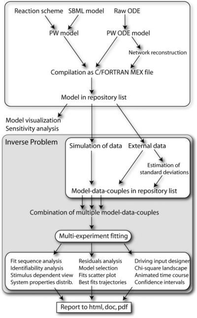
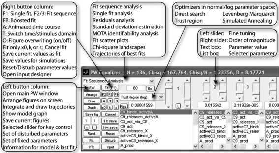
Figure 1 illustrates the workflow of modeling with PW. Either a biochemical reaction scheme is implemented by the modeler into a PW model definition file, or an SMBL model (Finney and Hucka, 2003) is imported. Alternatively, a raw set of ordinary differential equations (ODE) can be used to create a PW ODE model for which the reaction network can optionally be reconstructed. Loading of the model into the so-called repository list results in the compilation of a C/FORTRAN MEX file. Then, the model can be used for model visualization or methods of the direct problem, e.g. sensitivity analysis. In order to approach the inverse problem, one or more datasets have to be attached to the model either by simulation or from an external data source. Optionally, the SD of the data points can be estimated. Several model-data-couples can be combined for multi-experiment fitting. Afterwards, a variety of fit-based analyses are available investigating, for example, the identifiability and confidence intervals of the calibrated parameters. Finally, each analysis can be appended into an automatically generated report saved as a html, doc or pdf file. The central graphical user interfaces to operate within the workflow are the main PW window including a list of model-data-couples (Supplementary, Fig. 1) and the so-called Equalizer providing direct access to functionalities concerning the inverse problem (Fig. 2).

Fig. 1.

PW workflow as described in Section 2.1.

Fig. 2.

PW Equalizer. The PW Equalizer comprises 10 pairs of sliders. Each pair can be attached to one of the fitted parameters in the list box below the slider pair. The left slider is used for fine-tuning and the right slider changes the magnitude of the selected parameter. Text boxes on the one hand reflect the current parameter value and can on the other hand be used directly to specify a certain value. Thirty-three buttons and combo boxes provide direct access to the most important functions concerning multi-experiment fitting and analysis.

2.2 Creating an apoptosis example model

A realistic, medium sized model with 13 species, 41 reactions, and 13 kinetic parameters serves as an example to demonstrate the functionalities of PW. The model has been suggested by Legewie et al., (2006) and describes the feedback control of caspase-3 and caspase-9 in the intrinsic apoptosis signaling pathway (Supplementary, Fig. 3). The authors provided an SBML model which can be imported into PW. In order to investigate the increased statistical power to discriminate competing model hypothesis and to calibrate unknown parameters, we extended the model by two driving input functions representing an externally specified concentration of cyto-c and SMAC. The structure of the final model definition file is explained in the supplement comprising also an automatically generated model visualization.

2.3 Integration performance

During parameter calibration, the model trajectories have to be calculated thousands of times until an optimal parameter setting is found. Hence, high integration speed is a crucial prerequisite for interactive dynamical modeling of experimental data. PW applies the following strategy to meet these requirements:

1. Use of fast and accurate FORTRAN integrators.

2. The differential equations are saved and compiled as C MEX files. If possible, the integrator, interface and model are compiled into one single executable file.

3. The merit function is dynamically generated with improved numerical performance.

4. Calculation of observables and residuals is also based on dynamical C MEX files.

Currently, six FORTRAN integrators are supported by PW, being described in Hairer and Wanner (1996). We use the MATLAB interface of Ludwig, (2006), which we extended in two cases to increase speed by circumventing calls between integrator and the model equations. Our modification improves the integration time by an additional factor of 10–35. The integrators are RADAU5, RADAU, SEULEX, DOP853, DOPRI5 and ODEX. The first three integrators are applicable to stiff differential equations, where the time-scales of the variables have huge differences in their range. In order to compare the integration time and accuracy for a given model, PW supports all seven MATLAB integrators. A short description of each integrator can be found in the Supplementary Material.

The right hand side of the differential equations including algebraic equations, interpolation formulas and events is saved and compiled as a C MEX file when a model is loaded into PW. For the apoptosis model, this approach is 20 times faster than calling a MATLAB ODE function. We compare the performance of the 13 integrators by:

1. Total integration time.

2. Accuracy, measured as the averaged absolute distance of the integrated trajectory to a highly accurate integration with RADAU with 10⁻¹¹ absolute and 10⁻⁸ relative tolerance.

3. Number of calls of the right hand side of the ODE system.

4. Time per call of the right hand side.

The relative and absolute tolerances of the integration are usually set to 10⁻³ and 10⁻⁶, respectively. The RADAU integrator is tested with a variety of tolerances to illustrate the effect on integration time and on the number of calls to the ODE and to serve as a gold standard for the estimation of the integration accuracy. The integrations were applied on a Macintosh laptop with Intel Core 2 Duo 2.4 GHz with 2 GB RAM.

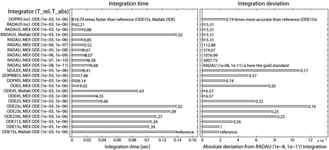
Figure 3 compares in detail the integration time and deviation for 23 different integration strategies. In summary, a compiled DOPRI5 including the ODE is approximately 900 times faster than using the reference MATLAB ode15s with a MATLAB ODE. If the ODE is not compiled into the integrator executable, DOPRI5 is still 26 times faster. Using RADAU5 that is applicable to stiff systems, an integration time 160 (incl. ODE) or 11 (attached ODE) times smaller than for the reference is achieved. Simultaneously, RADAU5 results in a five times smaller deviation than the reference compared to the trajectory of the gold standard. Figure 6 of the Supplementary Material compares the number of ODE calls and the time per call.

Fig. 3.

Integration time and accuracy. Left panel: the mean integration time of all 13 supported integrators with specified relative and absolute tolerance (T_rel, T_abs) is displayed. The integrator either includes the ODE (Rows 1 and 2) or is attached to an ODE compiled as C MEX file or saved as a normal MATLAB function. The reference is the MATLAB integrator ODE15s for stiff systems with a MATLAB ODE (last row, integration time 0.14 s, deviation 2×10⁻⁴). DOPRI5 for non-stiff systems is 919 times faster if the ODE is included (Row 1) and 26 times faster using a MEX ODE (Row 13). RADAU5, a stiff integrator, is 162 times faster with included ODE (Row 2) and 11 times faster with a MEX ODE (Row 3) compared to the reference. Increasing RADAU integration accuracy by 10⁻⁵ doubles the integration time (Rows 5–10). Right panel: integration with RADAU using high tolerances of 10⁻⁸ and 10⁻¹¹ serves here as a gold standard to estimate the accuracy of all integrators by quantifying the mean deviation between the calculated trajectories. RADAU5 (tolerances 10⁻³ and 10⁻⁶, Row 2) is not only faster than ODE15s, but also five times more accurate.

2.4 Optimization performance

The χ² merit function which is optimized within PW to fit the model y=y(t; p) is

(1)

with y_i being data point i with SD σ_i and y(t_i; p) being the model value at time point i for parameter values p. For normally distributed measurement errors, this corresponds to a Maximum Likelihood estimation (see Supplementary Material, Section 9.1). Five implementations of optimizers are available: direct search, trust region, Levenberg—Marquardt, genetic algorithm and simulated annealing. The direct search method (MATLAB; (Lagarias et al., 1998)) is only useful for illustration purposes or small models. The trust region (MATLAB optimization toolbox; (Coleman and Li, 1996)) and Levenberg–Marquardt (Nielsen, 2006) algorithms are powerful deterministic least-square optimizers. The simulated annealing (Ingber, 1989) and genetic algorithms (MATLAB genetic algorithm toolbox; (Goldberg, 1989)) are stochastic approaches able to handle local minima, but requiring more time. We quantify the accuracy of the optimization by the average deviation D of the n_p fitted parameters to the true parameters:

(2)

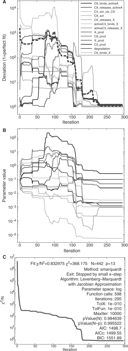
A deviation of value 1 indicates a perfect fit. A higher value indicates that on average the fitted value is D times higher than the true one or visa versa. Figure 4 exemplifies the result for the Levenberg–Marquardt algorithm. The initial guess for all parameters is the default value 0.1 corresponding to a mean deviation over 1000. After 598 function calls the deviation decreases to 1.0994, i.e. the parameters are on average only 10% higher or lower than the true values. This performance is based on the optimizer properties and on the PW framework allowing to fit in logarithmic parameter space, because the true parameter values span five orders of magnitude. Table 1 compares the results of Levenberg–Marquardt with trust region, simulated annealing, direct search and genetic algorithm. Optimization in normal parameter space was in no case successful, stressing the importance of fitting functionalities in logarithmic space. Please see the Supplementary Material for a detailed description of the performance analysis.

Fig. 4.

Optimization performance of Levenberg-Marquardt. (A): Deviation compared to true parameters. The mean deviation over all parameters (dashed red) reaches 1.0994 after around 240 iterations. After the final iteration, the maximum deviation was 1.30108, indicating that no parameter value differed more than 30% from the true value. (B): Parameter values during fitting. (C): χ²-value during fitting and fit settings.

Table 1.

Optimization performance

Optimizer	Deviation	Correct pars.	Fun. calls	Limits
Levenberg–Marquardt	1.0994	13/13	598	107
Trust region	1.0995	13/13	2184	107
Simulated annealing	12.62	12/13	10 323	400
Direct search	165807	5/13	7651	100
Genetic algorithm	188	3/13	40 000	103

Deviation of 1 corresponds to a perfect fit. Correctly determined parameters have a deviation below 30%. The required function calls are proportional to the fitting time. Limits around the true value are used during calibration stressing the high performance of the Levenberg–Marquardt and trust region optimizers.

2.5 Multi-experiment fitting

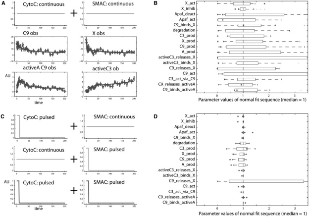
A key functionality of PW is multi-experiment fitting, where several datasets are fitted simultaneously. The datasets should derive preferably from different experimental conditions, e.g. different dose levels, pulses or ramp stimulations. The externally changed species, e.g. the ligand in models of signal transduction pathways, is called driving input. Figure 5 illustrates the power of multi-experiment fitting when applied to the apoptosis model. If only one experiment is available for model fitting with four observables and continuous stimulation by cyto-c and SMAC, the calibrated parameters possess a broad distribution with a relative SD often above 100% — they share non-identifiabilities. Including additional experiments with different combinations of pulsed and continuous stimulations resolves the non-identifiability for many parameters. In order to identify groups of parameters which are involved in a functional relationship, a fit sequence analysis reveals linear correlated pairs of parameters (see Supplementary Material, Fig. 16). Applying the incorporated MOTA algorithm ((Hengl et al., 2007)), also non-linear dependencies between an arbitrary number of parameters are detected. Altogether, nine parameters are affected by a non-identifiability, distributed in six groups with three to five parameters. Please, see the Supplementary Material for further details.

Fig. 5.

Application of multi-experiment fitting. If only one experiment with continuous stimulations for each driving input player cyto-c and SMAC (A), four observables, 10% rel.+10% absolute error, AU: arbitrary units) is fitted 200 times with varying initial guess for the parameters, the distributions of the calibrated parameter values is rather broad: the parameters are not identifiable (B). Combination of all four experiments (C) leads to significantly narrowed parameter distribution decreasing the relative uncertainty from over 100% to below 2% for 11 of 17 parameters (D). Note that the distribution represented by the horizontal bars should not be mistaken for a confidence interval (see Section 2.6). Therefore, true values (red stars) may lie outside of the parameter distributions.

2.6 Confidence intervals

Calculation of confidence intervals on the estimated parameter values requires that the parameters are identifiable. If a Maximum Likelihood estimator is used to calibrate the parameters, the confidence intervals can be determined based on the Hessian of the objective function at the optimum (Marsili-Libelli et al., 2003). Since PW uses a weighted least-square optimization, this is the case for normally distributed errors. Otherwise, a Monte-Carlo approach is preferable, where new datasets have to be generated based on the fitted model and an adequate observation error model (Press et al., 1999). PW supports both strategies, which are described in the Supplementary Material. The Supplementary Figure 20 demonstrates the difference between a normal fit sequence using the same dataset for fitting and a Monte-Carlo fit sequence.

2.7 Statistical tests

Two questions arise when experimental data is modeled:

1. Is the model statistically compliant with the data?

2. If two models are compliant with the data, which one should be taken?

In order to answer the firs question, usually the goodness-of-fit is determined, i.e. the distance between model and data is related to the expected value if the models were true: a χ²-test is applied (Press et al., 1999). For the second question, it is important to verify whether the models are nested, i.e. whether one model is an extension of the other model. In this case a likelihood-ratio test with high statistical power can be applied (Lehmann, 1986). Criteria like an Information Criterion (AIC) and Bayesian information criterion (BIC) are suggested to establish a ranking of models (Akaike, 1973; Schwartz, 1978). In the Supplementary Material, the methods are described in more detail and are applied to a reduced and enlarged apoptosis model, showing that the reduced model is significantly not compliant with the data. The extended model by construction sufficiently describes the data with a lower χ²-value than the original model. However, a likelihood ratio test reveals that the improvement is statistically not significant. The involved statistical functions are available in the PW framework.

2.8 Advanced modeling techniques

We shortly summarize which further modeling techniques are available within PW. Please see the Supplementary Materials for detailed descriptions. Model families allow for creating basis and dependent models in order to reduce redundant work, when the basis model is changed. Rules, start value assignments and events are algebraic equations evaluated during or before integration or when certain conditions are fulfilled. Basal states depending on parameter values require either sufficient integration before stimulation or should be set directly by start value assignments. Rule-based modeling is useful to cope with combinatorial complexity. Derived variables and parameters help to focus on important subsystems or to analyze functions of parameters. Soft constraints allow to include implicit algebraic equations or inequalities into the optimization. Delay reactions, based on the linear chain trick (MacDonald, 1976) are important for the modeling of black box elements, e.g. the time lag between translation and transcription. We determined the SD of the delay τ by means of Laplace transformation, which is described in the Supplementary Material. Residual analysis provides an additional means to validate the model-data-compliance based on distribution and auto-correlation properties. Automatic visualization is supported for the complete network or subsections. Network reconstruction can be applied to a set of differential equations with unavailable reaction scheme. A mapping dialog simplifies the coupling of model observation functions to external data files. Estimation of SDs for experimental data is based on smoothing splines. Powerful reporting facilities, means to store the workspace and saving of a model into the standard SBML format allows for efficient work and exchange of modeling results with collaborators.

3 DISCUSSION

PW is a comprehensive framework for data-based modeling in Systems Biology comprising multi-experiment fitting in normal and logarithmic parameter space. This is a crucial approach for model calibration in Systems Biology, where parameters are often spread over several orders of magnitude and systems can be observed only partially with relatively large measurement noise. Hessian- and Monte-Carlo-based calculation of confidence intervals are necessary to assess the possible range of the true parameter values.

PW integrates statistical tests for model-data-compliance, model discrimination and identifiability analysis for non-linear relationships between an arbitrary number of parameters. In order to resolve non-identifiabilities, we developed a user interface where characteristics of driving input functions corresponding to experimental conditions can be changed in real time. This could be applied in the context of experimental design as suggested in Maiwald et al., (2007) and Apgar et al., (2008). A variety of advanced modeling techniques is supported, as for example, consideration of implicit algebraic equations or inequalities during parameter calibration.

PW is a high-performance scientific yet user-friendly and customizable modeling framework. The program is tested for Windows, Linux and Mac systems and requires no special MATLAB toolboxes. PW is highly optimized through replacing time-crucial functions by new developed and existing C or FORTRAN code including just-in-time compilation. This increases integration speed up to 900 times compared to MATLAB integrators for a realistic benchmark system. We incorporated a fast Levenberg–Marquardt algorithm resulting in parameter calibration 3000 times faster than using MATLAB with the optimization toolbox. This is a crucial requisite for interactive real-time data-based modeling in Systems Biology and beyond.

REFERENCES

- Akaike H. Information theory and an extension of the maximum likelihood principle. In: Petrov B, Csaki F, editors. 2nd International Symposium on Information Theory. Budapest: Akademiai Kiado; 1973. pp. 267–281. [Google Scholar]
- Apgar JF, et al. Stimulus design for model selection and validation in cell signaling. PLoS Comput. Biol. 2008;4:e30. doi: 10.1371/journal.pcbi.0040030. [DOI] [PMC free article] [PubMed] [Google Scholar]
- Coleman TF, Li Y. An interior trust region approach for nonlinear minimization subject to bounds. SIAM J. Optim. 1996;6:418–445. [Google Scholar]
- Finney A, Hucka M. Systems biology markup language: level 2 and beyond. Biochem. Soc. Trans. 2003;31:1472–1473. doi: 10.1042/bst0311472. [DOI] [PubMed] [Google Scholar]
- Goldberg DE. Genetic Algorithms in Search, Optimization and Machine Learning. Boston, MA, USA: Addison-Wesley; 1989. [Google Scholar]
- Hairer E, Wanner G. Solving Ordinary Differential Equations II: Stiff and Differential algebraic Problems. New York: Springer, Berlin, Heidelberg; 1996. [Google Scholar]
- Hengl S, et al. Data-based identifiability analysis of non-linear dynamical models. Bioinformatics. 2007;23:2612–2618. doi: 10.1093/bioinformatics/btm382. [DOI] [PubMed] [Google Scholar]
- Hoops S, et al. COPASI–a complex pathway simulator. Bioinformatics. 2006;22:3067–3074. doi: 10.1093/bioinformatics/btl485. [DOI] [PubMed] [Google Scholar]
- Ingber L. Very fast simulated re-annealing. Math. Comput. Model. 1989;12:967–973. [Google Scholar]
- Klipp E, et al. Systems biology standards–the community speaks. Nat. Biotechnol. 2007;25:390–391. doi: 10.1038/nbt0407-390. [DOI] [PubMed] [Google Scholar]
- Lagarias J, et al. Convergence properties of the Nelder-Mead simplex method in low dimensions. SIAM J. Optim. 1998;9:112–147. [Google Scholar]
- Legewie S, et al. Mathematical modeling identifies inhibitors of apoptosis as mediators of positive feedback and bistability. PLoS Comput. Biol. 2006;2:e120. doi: 10.1371/journal.pcbi.0020120. [DOI] [PMC free article] [PubMed] [Google Scholar]
- Lehmann E. Testing Statistical Hypothesis. Berlin, Heidelberg, New York: Springer; 1986. [Google Scholar]
- Ludwig C. 2006. [(last accessed date July 30, 2008)]. MATLAB interface. Available at http://www-m3.ma.tum.de/twiki/bin/view/Software/ODEWebHome. [Google Scholar]
- MacDonald N. Time delay in simple chemostat models. Biotechnol. Bioeng. 1976;18:805–812. doi: 10.1002/bit.260180604. [DOI] [PubMed] [Google Scholar]
- Maiwald T, et al. Dynamic pathway modeling: feasibility analysis and optimal experimental design. Ann. N. Y. Acad. Sci. 2007;1115:212–220. doi: 10.1196/annals.1407.007. [DOI] [PubMed] [Google Scholar]
- Marsili-Libelli S, et al. Confidence regions of estimated parameters for ecological systems. Ecol. Model. 2003;165:127–146. [Google Scholar]
- Nielsen H. 2006. [(last accessed date July 30, 2008)]. Immoptibox. Available at http://www2.imm.dtu.dk/~hbn/immoptibox/ [Google Scholar]
- Press WH, et al. Numerical Recipes in C, The Art of Scientific Computing. 2nd. Cambridge, UK: Cambridge University Press; 1999. [Google Scholar]
- Schmidt H, Jirstrand M. Systems biology toolbox for matlab: a computational platform for research in systems biology. Bioinformatics. 2006;22:514–515. doi: 10.1093/bioinformatics/bti799. [DOI] [PubMed] [Google Scholar]
- Schwartz G. Estimating the dimension of a model. Ann. Stat. 1978;6:461–464. [Google Scholar]
- Tarantola A. Inverse Problem Theory and Model Parameter Estimation. Philadelphia: SIAM; 2004. [Google Scholar]
Associated Data
This section collects any data citations, data availability statements, or supplementary materials included in this article.