

Abstract
A fundamental problem in the analysis of protein folding and other complex reactions in which the entropy plays an important role is the determination of the activation free energy from experimental measurements or computer simulations. This article shows how to combine minimum-cut-based free energy profiles (FC), obtained from equilibrium molecular dynamics simulations, with conventional histogram-based free energy profiles (FH) to extract the coordinate-dependent diffusion coefficient on the FC (i.e., the method determines free energies and a diffusive preexponential factor along an appropriate reaction coordinate). The FC, in contrast to the FH, is shown to be invariant with respect to arbitrary transformations of the reaction coordinate, which makes possible partition of configuration space into basins in an invariant way. A “natural coordinate,” for which FH and FC differ by a multiplicative constant (constant diffusion coefficient), is introduced. The approach is illustrated by a model one-dimensional system, the alanine dipeptide, and the folding reaction of a double β-hairpin miniprotein. It is shown how the results can be used to test whether the putative reaction coordinate is a good reaction coordinate.
Keywords: diffusion, protein folding, one-dimensional free energy surfaces, variable diffusion coefficient
Free energy surface (FES) projected on a few progress variables (usually one or two) is often used to describe the equilibrium and kinetic properties of complex systems with a very large number (100 to 1,000 or more) of degrees of freedom. Studies of protein folding are an important example where this type of projected surface has been introduced and progress variables such as the number of native contacts and radius of gyration have been used (1–3). Most experimental analyses of protein folding have used a related approach; for example, if the distribution of folding times is exponential, it is assumed that there is a single free energy barrier along a generally unknown one-dimensional reaction coordinate. For a few systems that show more complex kinetics, the results have been interpreted in terms of projected FESs in two dimensions (4), although, again, the actual progress variables are not known. However, even when a one-dimensional single-barrier free energy projection seems adequate to describe the kinetics, there is a fundamental difficulty in determining the barrier height, because the measurements provide only one parameter (e.g., in protein folding, the rate constant of the corresponding unimolecular reaction is obtained). In such a standard “one-dimensional” analysis, the rate constant, k, is written as k = k0e−ΔF/kT, where k0 is the preexponential factor and ΔF is the free energy of activation. Thus, there are two unknowns, k0 and ΔF, to be determined from one measurement. For many small-molecule reactions, the entropic contribution to the barrier is negligible (ΔF ≈ ΔE, the activation energy), so that a measurement of the temperature dependence of the reaction rate can be used to find ΔE and k0, both assumed independent of temperature. However, for the protein-folding reaction and other reactions of complex systems, such as enzymatic reactions (5), the activation entropy plays an important role. As the protein folds, the loss of configurational entropy approximately cancels the stabilization of the native state by its lower energy (1), and the free energy barrier results from an imbalance between the two. Many discussions have been published concerned with the value of k0 to use for obtaining an estimate of ΔF from rate measurements. In particular, for reactions in solution and the large motions of the polypeptide chain involved in protein folding, a Kramers-type equation (6) with diffusive prefactors is appropriate. Such prefactors are much smaller than the Eyring value of kT/h (6 · 1012 at 300 K), standardly used for gas-phase reactions. Values of k0 on the order of 104 to 109 s−1 have been proposed (7–9). The “speed limit” for protein folding discussed by Kubelka et al. (10) essentially corresponds to a barrier-less reaction for which the rate is equal to the diffusion-limited rate coefficient. To summarize the experimental situation we quote from Yang and Gruebele (8): “Without sufficient knowledge of the critical reaction coordinate for describing the motion represented by ν+ [here k0] it is impossible to relate experimentally determined folding rates rigorously to computed free energy barriers.” A major aim of this article is to propose a method for solving this problem.
Theoretical studies based on simulations of the reaction rate for complex systems, such as peptides and proteins, often show simple exponential kinetics (11–13). To be able to determine both the preexponential factor and the free energy barrier from simulations, it is necessary to have a method of constructing the one-dimensional projected FES in terms of an appropriate reaction coordinate, if such exists. Given this projected surface and the calculated rate from simulations one can extract the rate coefficient and the free energy barrier. In a previous article (14) we showed how to use the minimum-cut procedure (11, 15) for finding free energy barriers and constructing one-dimensional free energy profiles (FEPs). In that article, we considered the ballistic regime (i.e., the quenching interval was large enough that the number of recrossings of the transition state was negligible). The free energy of the barrier was actually determined only up to an arbitrary additive constant corresponding to a preexponential factor, which is set equal to unity; that is, the minimum-cut value used for the free energy is equal to the total number of transition (i.e., proportional to the rate). Here we focus on the diffusive regime, which is implicit in Monte Carlo (MC) simulations and is valid in many cases for molecular dynamics (MD) simulations, as in protein-folding studies. In this regime, as we show in what follows, the FEP and diffusion coefficient as a function of the reaction coordinate can be evaluated separately.
In what follows we first demonstrate the essential results for a one-dimensional system to avoid complexity. We then outline how the results are generalized to the multidimensional case; for the practically important case of clustered equilibrium trajectories, the method corresponds to the minimum-cut procedure for the corresponding network (11, 14, 15). Applications are made to a transition of the alanine dipeptide and to the folding reaction of a double β-hairpin miniprotein, both simulated by MD with implicit solvent.
Methodology
FC and FH.
The conventional way to construct the projected FES is to perform equilibrium sampling of the configuration space (by MD or MC), select a progress variable (r), estimate the probability, P(r), to be in particular region of (r) by binning (making a histogram of) the results, and calculate the free energy as F(r) = −kT lnP(r); an absolute reference for the free energy can be used if a unique ground is known, as in lattice simulations (12). We refer to such histogram-based free energy projections as FH. By construction, the FH shows the probability of the system to have particular values of the chosen variable (r), from which all of the equilibrium properties as functions of this variable can be obtained. With the further assumption that the chosen coordinate is a “good” reaction coordinate (i.e., that the projection on this coordinate preserves the system kinetics) and that the motion on this surface can be described as diffusive along the reaction coordinates (3, 16), one can obtain information about the system's dynamics from the FH.
In many cases (11, 14), however, the standard progress variables (e.g., number of native contacts, radius of gyration) are not good reaction coordinates, because they do not preserve the barriers on the FES. Moreover, the diffusion coefficient is likely to vary in a complex way. Consequently, it is important for interpreting the simulated (or experimental) kinetics, as discussed in the introduction, to obtain the FEP as a function of a single coordinate that is a good reaction coordinate. One approach for doing this is to exploit an analogy between the system kinetics and equilibrium flow through a network (11, 14, 15). The essential element of this approach is to use the minimum-cut procedure for finding free energy barriers (11, 15) and, introducing the partition function as the reaction coordinate, to construct the FEP (14). The resulting free energy projections are referred to as “cut” FEPs (FC), in contrast to the FH. Other approaches for finding the reaction coordinates(s) for complex systems have been given in refs. 17–21.
On the basis of the calculated equilibrium trajectory, the partition functions of the bins of the FH are equal, ZH(i) = Σj nij = Ni, where nij is the number of transitions from bin j to bin i, and Ni is the number of times the system was found in bin i. The partition function of the cut used in the FC between two neighboring bins i and i + 1 is equal to ZC(i, i + 1) = ni,i+1. If there are transitions between more distant bins (i.e., the quench interval at which we observe the system is so large that transitions from nonneighboring clusters occur), one has to sum over them, so that ZC(i, i + 1) = Σj≤i<knjk. We note that although it is essential to bin the coordinate to construct the FH, the FC can, in principle, be obtained without binning. However, introduction of an equilibrium kinetic network (EKN), which does involve binning, is an efficient way to determine the FC for a multidimensional system (see The Multidimensional Case).
FC for Diffusive Motion.
In our previous works (11, 14, 15) we estimated the reaction rate between two basins as kij = Zij/Zj, where Zij is the detected number of transitions between two basins (found by the minimum-cut procedure) and Zj is the time the system spent in basin j. This measure is valid if the quench interval dt is longer than the time to diffuse through the transition state so that the number of recrossing events is negligible (“ballistic” regime) and, at the same time, dt is shorter than the mean lifetime in the basin so that the number of transition events that are left undetected, attributable to the system going back to the original basin, is negligible. If there is a separation between the two time scales, as is often true, the quench interval can be chosen to be between the two scales, and a meaningful description of the kinetics can be obtained (22, 23). To extend the analysis to the cases in which the recrossing is essential, we consider a reaction involving diffusive motion. For this purpose we focus on a one-dimensional system and treat a region of the FEP that is flat to a good approximation; that is, ZH(x) and D(x) are approximately independent of x, the reaction coordinate, in this region. This could be either a sufficiently small part of the FEP , so it does not change much, or an inherently flat part of the FEP, such as that in vicinity of a local maximum (e.g., a transition state) or minimum. The distance that the system moves during dt is distributed according to P(y) = (4πDdt)−1/2exp(−y2/4Ddt), the free-diffusion result. The number of jumps that cross the cut at x in one direction is equal to ZC(x) = ∫−∞0yP(y)ZH(x + y)dy = ZH(x)(Ddt/π)1/2 = 〈∣y∣〉 ZH/2, with ZH(x) the probability of finding the system at x, which is assumed to be constant in the interval of a few ; and 〈∣y∣〉 = ∫−∞∞P(y)∣y∣dy is the mean length the system moves during dt. Thus, D(x) = π/dt[ZC(x)/ZH(x)]2 together with ZH(x) give a complete description of the kinetics for a diffusive process. Because D(y) ∼ 〈Δy2〉/dt ∼ 〈(Δx dy/dx)2〉/dt ∼ D(x)(dy/dx)2 and ZH(y) = ZH(x)dx/dy, we obtain that ZC(y) = ZC(x) (i.e., FC is invariant for diffusive motion; see also below).
The reaction rate between two basins in the diffusive regime is equal to the reciprocal of the mean first passage time (mfpt; 〈t〉) from one basin to the other. The analytic equation for the mfpt from A to B given by 〈t〉 = ∫AB dxeβU(x)/D(x)∫Ax dye−βU(y), can be transformed to
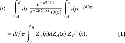 |
where ZA(x) = ∫Ax ZH(y)dy (i.e., the partition function corresponding to the reactant region, basin A).
Invariance of FC.
The FC is invariant, in contrast to the conventional FH, with respect to an arbitrary continuous invertible transformation of the coordinate space. Although we showed this above for the specific case of diffusive motion, the result is true generally. In one dimension for the FC, we have FC(y) = FC(x(y)), where F′(y) is the FEP with respect to the new coordinate y, and y(x) is the transformation. Thus, the transformation subjects the profile to arbitrary contraction or dilation along the coordinate axis in the one-dimensional case. Because the cut values are preserved (i.e., ni,i+1 remain the same), the local maxima and minima of the profile are preserved, and the partition of the configuration space into free energy basins is also invariant. For the FH, the total partition function, ZH(i) of the transformed image of the bin [i.e., the bin with borders yi = y(xi) and yi+1 = y(xi+1)] is also preserved. However, the bin size dyi changes so that the value of the mean partition function in the bin (yi < y < yi+1)ZH(y) = ZH(i)/dyi = ZH(x)dxi/dyi is changed. Consequently, the free energy is transformed as FH(y) = FH(x(y)) + kT ln(∣dy/dx∣), which means that the set of local minima and maxima is not invariant in the FH and that the partition of the configuration space into free energy basins can be altered.
This result has important practical consequences, because the FEPs are most commonly built by using putative reaction coordinates such as the number of native contacts or pfold (19, 22), which are highly nonlinear functions of the Cartesian configuration space through which the kinetics proceeds. On the basis of the FH in terms of such coordinates, the basins on the projected FES are determined, and the lowest pathways connecting them are obtained. This assumes implicitly that the diffusion coefficient is independent of the value of the reaction coordinate, which is not true in general. Because any coordinate system can be used to describe the kinetics (which is fully determined by FC and FH; see above), the changes in the FH must be compensated by changes in the diffusion coefficient as a function of the reaction coordinate to keep the FC constant; we give an example in An Example: Comparison of FH and FCfor a One-Dimensional Model System. The above result indicates that an important attribute of the FC, in contrast to the FH, is that different putative reaction coordinates can be used to analyze the FES because the barriers and minima are preserved.
Natural Coordinate.
One application of the invariance of the FC is that, knowing both FH and FC, it is straightforward to make a continuous invertible transformation to a coordinate y(x) such that they are proportional to each other; that is, that ZC(y)/ZH(y) = const (independent of y) and the diffusion coefficient is constant. We call such a coordinate a “natural” coordinate. Because ZC(x) = ZC(y) is invariant and ZH(y) = ZH(x)dx/dy, one obtains dy/dx = const × ZH(x)/ZC(x). A related but conceptually different approach to constructing such a coordinate on the basis of the FH specific for the case of pfold as the reaction coordinate was described recently by Rhee and Pande (16) [see supporting information (SI)].
Optimum One-Dimensional Projection.
It is reasonable to assume that any “bad” projection that results in overlapping of different parts of the configuration space will result in faster kinetics (i.e., in a smaller mfpt). Clearly, the longest mfpt is obtained on the original FES or from a projection where no such overlapping occurs. Hence, the maximum value of the integral in Eq. 1 can serve as a definition of the best one-dimensional projection. Taking ZA (the partition function of the reactant region) as the reaction coordinate (x) in Eq. 1 gives for the mfpt 〈t〉 = dt/π∫AB dZAZAZC−2(ZA). Assuming that the ZC(ZA) for different values of ZA are independent, the maximum 〈t〉 is attained when ZC(ZA) takes the minimal value for each value of ZA (i.e., the definition of the FEP introduced in ref. 14, which optimizes FC, maximizes the barrier as a function of ZA).
A referee pointed to a very interesting paper in a book (24) of which we were unaware. That paper also considers two types of FEPs: one is the standard one, identical with FH(q), and the other is related to, but different from, FC(q) except for a special case. We compare the two approaches in the SI.
An Example: Comparison of FH and FC for a One-Dimensional Model System
We use a simple model potential energy surface (PES), U(x) = −cos(x), with U(x) in units of kT and x in radians. For this one-dimensional system, the PES is the same as the FES and the FEP. The dynamics were simulated by performing MC sampling at a temperature (in energetic units of kT) equal to 0.5 for 107 steps, with the steps selected from a Gaussian distribution with zero mean and root-mean-square deviation (rmsd) of 0.1 (i.e., the diffusion coefficient is D = 〈Δx2〉/2Δt = 0.12/2). At quench interval of one step (dt = 1), the observed dynamics is in the diffusive regime because of the use of MC sampling. To compute the FH(x) we partitioned the x axis into bins of size of 0.01. The mean value of the partition function ZH(x) in bin i, associated with the point x, is equal to the number of times the system was found in this bin, divided by the size of the bin. The value of the partition function ZC(x) of the FC(x) at point x is equal to the number of times the system's trajectory crossed this point in one direction (or, for equilibrium sampling, in both directions divided by 2). With the relation F(x) = −kT ln(Z(x)), one obtains the FH(x) and FC(x).
Fig. 1 shows that FH(x) and FC(x) are essentially identical to U(x) except for the conventional additive constant. The FH(x) has slightly more noise in the regions of the maxima, where sampling is limited. We note that to build a histogram [FH(x)], one specifies a bin width that provides the optimum tradeoff between good statistics (large width) and good spatial resolution (small width). For the FC(x) there is no such problem; one can put surfaces arbitrarily close to each other, and one still obtains meaningful results. With a bin size of 0.001 (instead of 0.01) based on the same MC simulation, the FH(x) shows increased fluctuation, whereas the FC(x) does not (see Fig. 1B).
Fig. 1.

Model PES (= FES) U(x) = −cos(x) (solid line) together with reconstructed FC and FH. The distance between FC and FH is equal to kT ln() = 0.25ln(0.01/2/π) ≈ 1.61 (see below). (A) Bin size of 0.01. (B) Bin size of 0.001 (see text).
To illustrate the invariance of FC(x), the highly nonlinear transformation y(x) = x + sin(4x)/4 was chosen. Fig. 2A shows the result. Both the analytical transformation and the trajectory of the original MC simulation transformed to the new reaction coordinate were used to obtain the profiles; they are essentially identical. Although U(y) and the FC(y) change shape, the important point is that both still have two minima separated by a barrier. By contrast, the FH(y) has eight minima separated by seven barriers. For the present case, use of the angular coordinate x satisfies the condition that the FC(x) and the FH(x) be identical [up to a constant −kT log()] as shown in Fig. 1, whereas they are not for the transformed coordinate y(x). The diffusion constant obtained from D(y) = D(x)(dy/dx)2 mirrors the transformed FH(y) (see Fig. 2A).
Fig. 2.

Transformations of the FEPs. (A) Model PES and reconstructed FEPs along the coordinate y(x) = x + sin(4x)/4. The lines are (top to bottom) −kT ln(D(y)), where D(y) is the diffusion constant as function of y, U(x(y)), FC, and FH. (B) FC (and FH) from A transformed “back” to natural coordinate z.
Fig. 2B shows the FC(z) [the FH(z) is not shown, because it coincides with FC(z) by construction] along the natural coordinate z, where dz/dy = ZH(y)/ZC(y), and ZC(y) and ZH(y) correspond to the FC(y) and FH(y) shown in Fig. 2A. The FC(z) along the natural coordinate z is identical to that in Fig. 1 except that the x axis is more extended, whereas the ZC(x) and ZH(x) differ by a multiplicative constant (D/π)1/2 in Fig. 1; they are identical in Fig. 2B.
For this model system, Eq. 1 gives values for the mfpt 〈t〉 between 49,781 and 46,100 steps for dt = {20…28}, which is in agreement with value of 47,169 steps found from the MC simulation. Instead of comparing mfpts, one can compare the effective number of transitions between the basins, estimated via the mfpt as nij = nji = Zj/〈tij〉, and determined directly by counting the number of transitions between the basins in the trajectory. For dt = 1, the numbers are 95.6 and 106, respectively. The statistical uncertainty (variance) of the number of transitions estimated via the mfpt is half as large as the one obtained by actual counting; for example, the variances estimated with the trajectory divided into 10 pieces, 106 steps each, are 1.6 and 3.4, respectively.
The relation between FC and FH [ZC = ZH(Ddt/π)1/2], derived above, is valid for inherently diffusive motion, as described by MC dynamics. For MD the motion can also be diffusive (e.g., as it is in most cases of protein folding), but on a short time scale (when the stochastic approximation is not yet valid) the motions are essentially ballistic so that Δx ∼ vdt and ZC ∼ ZHvdt. If one examines a trajectory and changes only dt during the analysis, then, because ZH ∼ 1/dt, ZC ∼ (D/dt)1/2 in the diffusive regime. This is in contrast with ZC ∼ const for the ballistic regime and can be used, therefore, to distinguish the two regimes.
The dependence of the FC on dt for the model potential is discussed in the SI.
Alanine Dipeptide.
The kinetics of the alanine dipeptide was simulated with the CHARMM program (25) by using the polar hydrogen force field (26) with the ACE2 implicit solvent model (27) for 108 steps; each step was 2 fs. A temperature of 400 K was used to ensure coverage of the important regions of the FES; the temperature was controlled by a Nose–Hoover thermostat.
Fig. 3A shows the FC(φ) along the φ dihedral angle obtained with various quench time intervals. For dt = 1, 2, 4 MD steps, the FC is approximately constant (i.e., the motion is ballistic). For dt = 8 MD steps, FC changes by a constant (i.e., the motion starts to deviate from ballistic and can be approximately described as diffusive). This is supported by the fact that the difference between FC(φ) for dt = 8 and dt = 64 is approximately constant and equal to 0.8, which is close to the exact value of kT ln(8)/2 = 0.83 for diffusive motion. Nonmonotonic changes in the distances between the FEPs arise from the fact that motion is not completely stochastic and some correlations are still present.
Fig. 3.

FEPs for alanine dipeptide. (A) FC along the φ dihedral angle for various quench time intervals dt (given in MD steps). (B) FC and FH along the φ and ψ dihedral angles.
Fig. 3B shows the FC and FH along the φ and ψ dihedral angles. There is a notable difference between the profiles, with the difference depending on the angle, which indicates that the diffusion coefficient is not constant. The difference between FC and FH for both angles (data not shown) can be approximated by a + bcos(φ) [a + bcos(ψ)] with b ≈ 0.4 kcal for φ and b ≈ 0.35 kcal for ψ.
The analysis has shown that the dynamics of the dipeptide along the dihedral angles can be considered to be diffusive for time steps of ≥8 fs with a diffusion coefficient [determined as D(x) = π/dtZC2(x)/ZH2(x) for dt = 8 fs] ranging from 3 deg2/fs (at angle values close to ±180) to 7 deg2/fs (at angle values close to 0). The mfpt to go from C7eq (φ = −79, ψ = 133) to the C7ax (φ = 63, ψ = −77) as estimated with Eq 1, based on the calculated profile for dt = 8 fs, is equal to 3.8 · 106 steps. The result is in good agreement with the number (3.9 · 106 steps) obtained by direct counting (based on 24 transitions). It indicates that φ alone is a good reaction coordinate for describing transition between C7eq and C7ex. This behavior is somewhat surprising, because there are two major transition states on the alanine dipeptide FES for this transition: the associated (φ, ψ) values are (φ = 1, ψ = −71) and (φ = 9, ψ = 89) (28). Because the φ values are nearly the same, they match in the φ projection, resulting in the highest possible (correct) single barrier.
The usual harmonic approximation in the Kramers formulation (29) for the mfpt is 〈t〉 = 2π/(βωω†D†)exp(βΔG) = 2π/(βωω†D†)ZH/ZH† (where † denotes the values at the transition state). By introducing the expression for the diffusion coefficient D = π/dt(ZC/ZH)2, the equation can be transformed to
Using the values of ω = 0.04 and ω† = 0.077 obtained by fitting the potential in Fig. 3B, we obtain 〈t〉 = 3.2 · 106 steps. If one takes account of the anharmonicity of the ground state, 〈t〉 = 3.5 · 106 steps, which is in good agreement with the exact results.
The Multidimensional Case
Generalization of the FC-based approach to the multidimensional case is straightforward, in principle, because ZC(S) is defined for every surface S in configurational space as the number of transitions through it. However, the specification of the surface in the multidimensional space is evidently more complex than that in the one-dimensional case. The invariance to an arbitrary continuous invertible transformation of configurational space remains valid, because the number of transitions through the surface is preserved. To find the ensemble of transition states between two points, one determines the surface with the minimal partition function that separates these two points (15, 30). However, when one approximates the flow by a finite trajectory, one has to take into consideration the fact that for a configuration space of more than two dimensions the trajectory essentially never crosses itself. Thus, one can always find a surface that separates any two points and crosses the trajectory only once. To avoid this problem one can coarse-grain the space and gather nearby points of the trajectory into clusters, based on an appropriate criterion (e.g., rmsd, secondary structure strings, number of native contacts). This leads to an EKN consisting of a set of states and the transitions between them (14). Instead of specifying the cutting surface, one then needs only list the edges of the network, which are cut by the surface. The flow over the surface is mapped onto the cuts of the network; the minimum cut is used to find the links corresponding to the transition-state ensemble (15).
Folding of the Beta3s Miniprotein.
Folding of the 20-residue Beta3s double-hairpin miniprotein has been studied (31, 32), based on a 20-ms equilibrium trajectory calculated with the solvent-accessible surface area implicit solvent model (33). Detailed analyses of the folding behavior of this system and its folding network were made. Secondary structure clustering and rmsd clustering with an all-atom rmsd of 2.5 Å were compared, and it was shown that the basins on the FEP obtained from the two types of clustering were in good agreement. However, it was found that folding rate was faster by almost an order of magnitude in the case of secondary structure clustering than that obtained with rmsd clustering. To interpret this result we consider the dependence of FEPs obtained with the two types of clustering on the quench interval dt. Snapshots of trajectory taken with quench interval dt were clustered into an EKN and the FEPs were constructed with the pfoldf algorithm (14). Fig. 4A shows the FEPs obtained with rmsd 2.5-Å clustering. Increasing the quench interval generally leads to a less connected network; thus, the profile for dt = 2 has more noise. However, the dt = 2 profile is almost equidistant from the dt = 1 profile, with a spacing of 0.35(ln()); that is, the profiles are proportional to dt−1/2, consistent with the diffusive regime. Use of either profile gives the same value for the diffusion coefficient and leads to the same temporal behavior.
Fig. 4.

FC/kT = −ln(ZC) for dt = 1, 2 for Beta3s. (A) rmsd clustering with a 2.5-Å cutoff radius shows dt−1/2 behavior. (B) Secondary structure clustering shows dt−1 behavior. For brevity we show just the part of the FEP 0 < ZA/Z < 0.6. The native state occupies the region 0 < ZA/Z < 0.35, followed by the denatured state, which includes several enthalpic basins.
Fig. 4B shows the FEPs obtained with secondary structure clustering. The profiles are also almost equidistant with distance of 0.7(ln(2)); that is, the profiles are proportional to dt−1, which is inconsistent with the diffusive regime. The profile obtained with a larger dt has a smaller diffusion coefficient (D ∼ ZC2/ZH2/dt ∼ dt−2/dt−2/dt ∼ dt−1) and, thus, exhibits slower kinetics. The dt−1 behavior can be explained if one supposes that with the secondary structure clustering, “shortcuts” between different parts of configuration space are possible (i.e., particular secondary structure strings correspond to significantly different configurations). Each such shortcut corresponds to a jump (with length independent of dt). Thus, ZC(x) = 〈∣y∣〉 ZH(x)/2 ∼ dt−1 (see above), where 〈∣y∣〉 is the mean length of the jump. The analysis leads to the conclusion that rmsd clustering is appropriate for the kinetics of folding of Beta3s, whereas secondary structure clustering introduces a significant number of shortcuts, making the description of the system kinetics as a diffusive process inconsistent (i.e., profiles obtained at different quench intervals lead to different behavior).
The advantage of the secondary structure clustering over the rmsd clustering is a small running time that increases linearly with trajectory size, whereas that for the latter grows quadratically. We suggest the following simple clustering method, which combines strong points of both methods. The configurations are in the same cluster only when they have equal secondary structures and their rmsd is less than the given threshold. Thus, rmsd is calculated only between configurations with equal secondary structures (i.e., the latter is used a hash function). Tests on the Beta3s miniprotein showed that the proposed clustering method is at least two orders of magnitude faster than rmsd and provides FEPs consistent with diffusive dynamics, unlike using secondary structure clustering alone.
Concluding Discussion
This article examines the properties of minimum-cut-based FEP (FC) and shows, in particular, that in the diffusive regime the diffusion coefficient (possibly coordinate-dependent) can be obtained directly from the FC and, together with the histogram-based free energy profile (FH), provides a complete description of the kinetics and the equilibrium properties. This makes possible the decomposition of the calculated rate into a preexponential factor (diffusion coefficient) and a free energy of activation. Alternatively, one can obtain the preexponential factor from k0 = eβΔF〈t〉−1, where 〈t〉 is the mfpt from the analytical solution and ΔF is the FC barrier height. An important property of the FC is that they are invariant under an arbitrary invertible transformation of the reaction coordinate, which means that the FC can be used, in contrast to FH, to partition the FES into basins in an invariant way (i.e., the number of barriers and minima and their heights along any appropriate reaction coordinate should be the same). By comparing the calculated kinetics with that obtained directly from the simulation, one can test whether the reaction coordinate used to project the FES is appropriate. For example, one can compare the mfpt found from simulations with that obtained from the standard analytical solution for one-dimensional diffusion. Moreover, the FC is less sensitive than the FH to limited statistics (i.e., there is no “tradeoff” between accuracy and resolution for the FC, in contrast to FH).
The partition function is introduced as a reaction coordinate, because it is among the simplest and most flexible coordinates that increase monotonically as the system goes from the initial to the final state. If there are several well defined pathways, this reaction coordinate will adapt its shape to them and progress mainly along the pathways (see an example in figure 5 of ref. 14). If the FEP is accurate, it describes the essence of the reaction kinetics by showing the barriers and basins on the way from the initial to the final state. Because the chosen progress coordinate is very flexible, the obtained FEP is likely to be the best way of projecting the FES onto a one-dimensional coordinate (see about Optimum One-Dimensional Projection above). Moreover, although the partition function may seem abstract (as does pfold, but see ref. 18), one can identify the structures associated with most important pathways by postprocessing the profiles.
Finally, we mention that recently there has been increasing discussion of the fact that reactions that in the past had been described in terms of a one-dimensional FES [e.g., enzymatic reactions (34) or the analysis of single-molecule experiments (35)] in fact require more than one dimension for a valid description. Although we have illustrated the present methodology by applying it to protein folding, we note that the approach is perfectly general. There may be practical limitations introduced by the difficulty of obtaining the necessary data. Nevertheless, the concept that it is possible to introduce a one-dimensional FES that contains all of the information necessary to describe the kinetics of reactions in complex systems should make the present approach of widespread interest. By considering time series of FRET efficiency, for example, one can obtain an invariant FEP together with the coordinate-dependent diffusion coefficient. The approach also suggests that the biasing potential in adaptive biased simulation (e.g., adaptive umbrella sampling) should be applied to “flatten” the invariant quantity FC, instead of FH, to speed up the kinetics of equilibration.
Supplementary Material
Acknowledgments.
We thank Amedeo Caflisch and his coworkers, who performed the long Beta3s simulation. The part of the research performed at Harvard was supported by a grant from the National Institutes of Health. S.V.K. is supported by the CHARMM Development Project.
Footnotes
The authors declare no conflict of interest.
This article contains supporting information online at www.pnas.org/cgi/content/full/0800228105/DCSupplemental.
References
- 1.Dobson CM, Sali A, Karplus M. Protein folding: A perspective from theory and experiment. Angew Chem Int Ed. 1998;37:868–893. doi: 10.1002/(SICI)1521-3773(19980420)37:7<868::AID-ANIE868>3.0.CO;2-H. [DOI] [PubMed] [Google Scholar]
- 2.Shea JE, Brooks CL. From folding theories to folding proteins: A review and assessment of simulation studies of protein folding and unfolding. Annu Rev Phys Chem. 2001;52:499–535. doi: 10.1146/annurev.physchem.52.1.499. [DOI] [PubMed] [Google Scholar]
- 3.Onuchic JN, Socci ND, Luthey-Schulten Z, Wolynes PG. Protein folding funnels: The nature of the transition state ensemble. Fold Des. 1996;1:441–450. doi: 10.1016/S1359-0278(96)00060-0. [DOI] [PubMed] [Google Scholar]
- 4.Sabelko J, Ervin J, Gruebele M. Observation of strange kinetics in protein folding. Proc Natl Acad Sci USA. 1999;96:6031–6036. doi: 10.1073/pnas.96.11.6031. [DOI] [PMC free article] [PubMed] [Google Scholar]
- 5.Karplus M. Aspects of protein reaction dynamics: Deviations from simple behavior. J Phys Chem B. 2000;104:11–27. [Google Scholar]
- 6.Kramers HA. Brownian motion in a field of force and the diffusion model of chemical reactions. Physica. 1940;7:284–304. [Google Scholar]
- 7.Hagen SJ, Hofrichter J, Szabo A, Eaton WA. Diffusion-limited contact formation in unfolded cytochrome c: Estimating the maximum rate of protein folding. Proc Natl Acad Sci USA. 1996;93:11615–11617. doi: 10.1073/pnas.93.21.11615. [DOI] [PMC free article] [PubMed] [Google Scholar]
- 8.Yang WY, Gruebele M. Folding at the speed limit. Nature. 2003;423:193–197. doi: 10.1038/nature01609. [DOI] [PubMed] [Google Scholar]
- 9.Chan HS, Dill KA. Protein folding in the landscape perspective: Chevron plots and non-Arrhenius kinetics. Proteins. 1998;30:2–33. doi: 10.1002/(sici)1097-0134(19980101)30:1<2::aid-prot2>3.0.co;2-r. [DOI] [PubMed] [Google Scholar]
- 10.Kubelka J, Hofrichter J, Eaton WA. The protein folding “speed limit.”. Curr Opin Struct Biol. 2004;14:76–88. doi: 10.1016/j.sbi.2004.01.013. [DOI] [PubMed] [Google Scholar]
- 11.Krivov SV, Karplus M. Hidden complexity of free energy surfaces for peptide (protein) folding. Proc Natl Acad Sci USA. 2004;101:14766–14770. doi: 10.1073/pnas.0406234101. [DOI] [PMC free article] [PubMed] [Google Scholar]
- 12.Palyanov AY, Krivov SV, Karplus M, Chekmarev SF. A lattice protein with an amyloidogenic latent state: Stability and folding kinetics. J Phys Chem B. 2007;111:2675–2687. doi: 10.1021/jp067027a. [DOI] [PubMed] [Google Scholar]
- 13.Socci ND, Onuchic JN, Wolynes PG. Diffusive dynamics of the reaction coordinate for protein folding funnels. J Chem Phys. 1996;104:5860–5868. [Google Scholar]
- 14.Krivov SV, Karplus M. One-dimensional free-energy profiles of complex systems: Progress variables that preserve the barriers. J Phys Chem B. 2006;110:12689–12698. doi: 10.1021/jp060039b. [DOI] [PubMed] [Google Scholar]
- 15.Krivov SV, Karplus M. Free energy disconnectivity graphs: Application to peptide models. J Chem Phys. 2002;117:10894–10903. [Google Scholar]
- 16.Rhee YM, Pande VS. One-dimensional reaction coordinate and the corresponding potential of mean force from commitment probability distribution. J Phys Chem B. 2005;109:6780–6786. doi: 10.1021/jp045544s. [DOI] [PubMed] [Google Scholar]
- 17.Best RB, Hummer G. Reaction coordinates and rates from transition paths. Proc Natl Acad Sci USA. 2005;102:6732–6737. doi: 10.1073/pnas.0408098102. [DOI] [PMC free article] [PubMed] [Google Scholar]
- 18.Ma A, Dinner AR. Automatic method for identifying reaction coordinates in complex systems. J Phys Chem B. 2005;109:6769–6779. doi: 10.1021/jp045546c. [DOI] [PubMed] [Google Scholar]
- 19.Du R, Pande VS, Grosberg AY, Tanaka T, Shakhnovich ES. On the transition coordinate for protein folding. J Chem Phys. 1998;108:334–350. [Google Scholar]
- 20.Das P, Moll M, Stamati H, Kavraki LE, Clementi C. Low-dimensional, free-energy landscapes of protein-folding reactions by nonlinear dimensionality reduction. Proc Natl Acad Sci USA. 2006;103:9885–9890. doi: 10.1073/pnas.0603553103. [DOI] [PMC free article] [PubMed] [Google Scholar]
- 21.Mu Y, Nguyen PH, Stock G. Energy landscape of a small peptide revealed by dihedral angle principal component analysis. Proteins. 2005;58:45–52. doi: 10.1002/prot.20310. [DOI] [PubMed] [Google Scholar]
- 22.Chandler D. Statistical mechanics of isomerization dynamics in liquids and the transition state approximation. J Chem Phys. 1978;68:2959–2970. [Google Scholar]
- 23.Chandler D. Introduction to Modern Statistical Mechanics. New York: Oxford Univ Press; 1987. p. 288. [Google Scholar]
- 24.E W, Vanden-Eijnden E. Metastability, conformational dynamics, and transition pathways in complex systems. In: Attinger S, Koumoutsakos P, editors. Multiscale Modelling and Simulation. Springer; 2004. pp. 277–312. [Google Scholar]
- 25.Brooks BR, et al. CHARMM: A program for macromolecular energy, minimization, and dynamics calculations. J Comput Chem. 1983;4:187–217. [Google Scholar]
- 26.Neria E, Fischer S, Karplus M. Simulation of activation free energies in molecular systems. J Chem Phys. 1996;105:1902–1921. [Google Scholar]
- 27.Schaefer M, Bartels C, Karplus M. Solution conformations and thermodynamics of structured peptides: Molecular dynamics simulation with an implicit solvation model. J Mol Biol. 1998;284:835–848. doi: 10.1006/jmbi.1998.2172. [DOI] [PubMed] [Google Scholar]
- 28.van der Vaart A, Karplus M. Simulation of conformational transitions by the restricted perturbation-targeted molecular dynamics method. J Chem Phys. 2005;122:114903. doi: 10.1063/1.1861885. [DOI] [PubMed] [Google Scholar]
- 29.Levy RM, Karplus M, McCammon JA. Diffusive Langevin dynamics of model alkanes. Chem Phys Lett. 1979;65:4–11. [Google Scholar]
- 30.Truhlar D, Garrett B, Klippenstein S. Current status of transition-state theory. J Phys Chem. 1996;100:12771–12800. [Google Scholar]
- 31.Ferrara P, Caflisch A. Folding simulations of a three-stranded antiparallel β-sheet peptide. Proc Natl Acad Sci USA. 2000;97:10780–10785. doi: 10.1073/pnas.190324897. [DOI] [PMC free article] [PubMed] [Google Scholar]
- 32.Rao F, Caflisch A. The protein folding network. J Mol Biol. 2004;342:299–306. doi: 10.1016/j.jmb.2004.06.063. [DOI] [PubMed] [Google Scholar]
- 33.Ferrara P, Apostolakis J, Caflisch A. Evaluation of a fast implicit solvent model for molecular dynamics simulations. Proteins. 2002;46:24–33. doi: 10.1002/prot.10001. [DOI] [PubMed] [Google Scholar]
- 34.Benkovic SJ, Hammes GG, Hammes-Schiffer S. Free-energy landscape of enzyme catalysis. Biochemistry. 2008;47:3317–3321. doi: 10.1021/bi800049z. [DOI] [PubMed] [Google Scholar]
- 35.Min W, Xie X, Bagchi B. Two-dimensional reaction free energy surfaces of catalytic reaction: Effects of protein conformational dynamics on enzyme catalysis. J Phys Chem B. 2008;112:454–466. doi: 10.1021/jp076533c. [DOI] [PubMed] [Google Scholar]
Associated Data
This section collects any data citations, data availability statements, or supplementary materials included in this article.