Organizing Principles of Spectro-Temporal Encoding in the Avian Primary Auditory Area Field L

Abstract

The organization of post-thalamic auditory areas remains unclear in many respects. Using a stimulus based on properties of natural sounds, we mapped spectro-temporal receptive fields (STRFs) of neurons in the primary auditory area field L of unanesthetized zebra finches. Cells were sensitive to only a subset of possible acoustic features: nearly all neurons were narrowly tuned along either the spectral dimension, the temporal dimension, or both; broadly tuned and strongly orientation-sensitive cells were rare. At high stimulus intensities, neurons were sensitive to differences in sound energy along their preferred dimension, while at lower intensities, neurons behaved more like simple detectors. Finally, we found a systematic relationship between neurons’ STRFs, their electrophysiological properties, and their location in field L input or output layers. These data suggest that spectral and temporal processing are segregated within field L, and provide a unifying account of how field L response properties depend on stimulus intensity.

Introduction

Understanding how complex stimuli are decomposed and represented by populations of neurons is a central goal of sensory neuroscience. In visual cortex, cells are tuned to orientation, and have response properties that depend on their spatial position within a column (e.g. Hubel and Wiesel, 1962). In the auditory brainstem, parallel pathways encode the timing, intensity, and frequency of incoming sounds in ways that depend on the electrical, synaptic, and morphological properties of different cell populations (e.g. Rhode and Smith, 1983, 1987; Oertel 1991, Sullivan, 1985).

At higher levels of the auditory system, the organizing principles are less clear. Until recently, responses to different sound frequencies and responses to slow amplitude modulations in time were generally studied separately (Phillips and Irvine, 1981; Phillips and Hall, 1987; Schreiner et al., 1992; Schreiner et al., 1997; Lu et al., 2001; Liang et al., 2002; Barbour and Wang, 2003). More recently, reverse correlation approaches have made it possible to measure spectral and temporal response properties together (Miller et al., 2002; Depireux et al., 2001; Kowalski et al., 1996, 1997, Theunissen et al., 2000; Sen et al., 2001; Woolley et al., 2005, 2006). While such studies have begun to identify differences in auditory selectivity between areas (Sen et al., 2001; Miller et al., 2002; Linden et al., 2003), they have chiefly revealed a diversity of response types, and few clear links between response properties, cellular properties, and anatomy have emerged.

The songbird provides an excellent model system to study the neural representation of complex sounds. Songbirds produce and perceive complex learned sounds that share many acoustic features with human speech (Singh and Theunissen, 2003). The songbird forebrain contains a primary auditory area known as field L that is analogous to the primary auditory cortex of mammals, and forms a gateway for auditory information to reach forebrain areas involved in song production and recognition (Wild et al., 1993; Fortune and Margoliash, 1995). Studies using simple tone stimuli have identified multiple tonotopic maps in the field L complex (Scheich et al., 1979; Heil et al., 1985; Gehr et al., 1999, Terleph et al., 1996), while anatomical studies have identified 3 layers (L1, 2, and 3) that differ in their connectivity and cyto-architecture (Fortune and Margoliash, 1992). Layer L2 receives thalamic input, while L1 and L3 project to higher auditory areas (Wild et al., 1993; Vates et al., 1996). Recent studies have compared response properties across field L layers (Sen et al., 2001), and between field L and surrounding auditory regions (Muller and Leppelsack, 1985, Lewicki and Arthur 1996, Woolley et al., 2005, 2006), but have not described the distribution of single cell responses in detail, nor linked these response properties to cell types.

In this study, we used a rich synthetic stimulus and reverse-correlation techniques (Eggermont et al., 1983; Depireux et al., 2001; Kim and Rieke, 2001, Miller et al., 2002; Escabi and Schreiner 2002; Theunissen et al., 2000) to measure spectro-temporal receptive fields (STRFs) in field L of unanesthetized animals. We found that field L neurons show sensitivity to only a subset of possible acoustic features, and that they change in systematic ways with stimulus intensity. Different layers of field L show differences both in their acoustic response properties and their electrophysiology. These data provide new insights into the organization of a higher-level auditory area.

Results

Stimulus Design

To identify the spectro-temporal features that drive cells in field L, we designed a stimulus that sampled time and frequency combinations in an unbiased way. The stimulus consisted of 32 logarithmically spaced frequency bands (figure 1A, column 1), each modulated by a different time-varying amplitude envelope (column 2), then summed to produce the final signal (column 3). The envelopes were designed such that the log amplitude of each band was a random Gaussian noise signal with an exponential distribution of frequencies. Envelopes were statistically identical to those used in a previous experiment (Nagel and Doupe, 2006). Frequency bands were Gaussian in log-frequency and overlapped by one standard deviation. Full details of the stimulus construction are given in Methods.

Figure 1. Construction of a stimulus with a naturalistic distribution of spectral and temporal modulation frequencies.

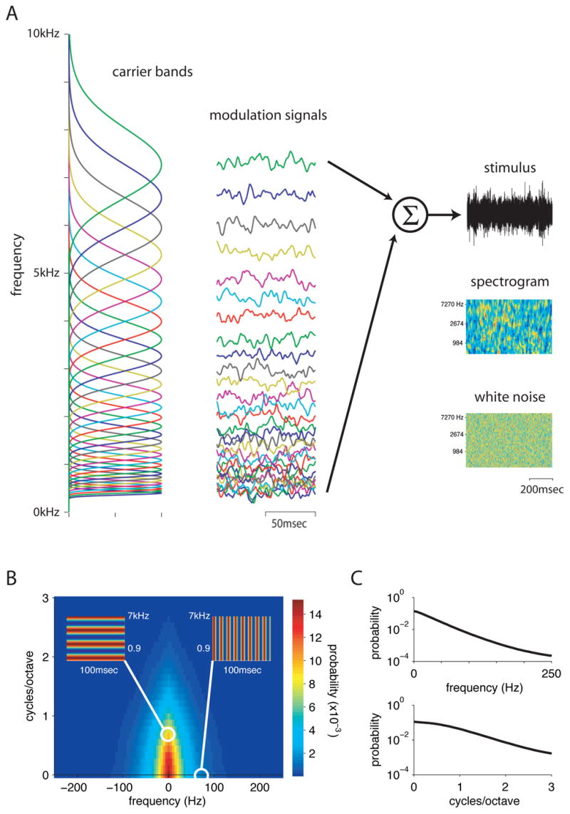
A) Schematic of stimulus construction. 32 overlapping frequency bands (left-hand column) were modulated by independent envelopes (column 2). The stimulus was the sum of these bands, shown as both an oscillogram (sound pressure as a function of time, top panel) and as a spectrogram (frequency content versus time, 2nd panel) in the right hand column. The naturalistic stimulus was smoother in both time and frequency than a pure white noise stimulus (bottom panel).

B) Quantitative analysis of stimulus correlations. The two-dimensional modulation spectrum of the stimulus shows the distribution of energy in the stimulus as a function of temporal modulation frequency (x-axis) and spectral modulation frequency (y-axis). Pure spectral modulations (left inset) and pure temporal modulations (right inset) are represented along the y and x axes respectively.

C) Marginal distributions show stimulus energy on a log axis as a function of temporal frequency (top panel) or of spectral frequency (bottom panel). These indicate that energy in the stimulus is concentrated at low temporal and spectral modulation frequencies, but has tails that reach to higher frequencies.

As a result of its construction, the frequency content of our stimulus varied randomly and smoothly in time. This can be seen in the spectrogram of the stimulus (3rd column, 2nd panel), which shows the intensity of sound at each frequency as a function of time. Frequency peaks in the stimulus are broader and last longer than those in the white noise spectrogram below it. Local correlations like those in our stimulus are found in most natural sounds, including song, speech, and environmental noise (Singh and Theunissen, 2003). They enabled our stimulus to drive field L neurons more effectively and reliably than white noise (data not shown).

The correlations in the stimulus can be quantified by plotting its modulation spectrum (figure 1B, Singh and Theunissen, 2003). This heat map shows the energy in the stimulus as a function of temporal and spectral frequency. Temporal features of sound, such as syllable onsets and offsets, give rise to energy along the x-axis. Spectral features, such as harmonic combinations, give rise to energy along the y-axis. Energy off the axes represents joint spectro-temporal features, such as upward and downward frequency sweeps. Asymmetry between the two halves would indicate that upward or downward sweeps predominated in the stimulus, while the symmetric distribution seen here indicates that they were equally likely. Although our stimulus is dominated by low spectral and temporal frequencies, it contains small, gradually decreasing amounts of energy at higher frequencies. These high frequency tails can be seen in log-scaled marginal distributions (figure 1C) of stimulus energy as a function of temporal or spectral frequency alone.

The distribution of energy in our synthetic stimulus shares many features with the statistics of natural sounds such as song and speech. Natural sounds also have most of their energy at low spectral and temporal modulation frequencies, with a long tail of higher frequencies; their temporal and spectral modulation spectra can be approximated by a power law (Singh and Theunissen, 2003). Compared to our stimulus, zebra finch song and speech have energy more tightly concentrated along the x and y axes of the modulation spectrum (see Singh and Theunissen, 2003, Hsu et al., 2004, figure 1, Woolley et al., 2005, figure 1), indicating that they consist largely of pure spectral features (such as the harmonic combinations found in vowels) and pure temporal features (such as the amplitude modulations found in consonants).

STRFs were obtained by calculating the average spectrogram preceding a spike, then “decorrelating” the resulting spike-triggered average (see Methods). STRFs estimated from true natural stimuli (Sen et al, 2001; Machens et al, 2004; Ringach et al, 2002) can be distorted by high order stimulus correlations not captured by the modulation spectrum (Sharpee et al 2004). Our stimulus had a known correlation structure, ensuring that the influence of such correlations on our STRFs could be removed through decorrelation. Decorrelation generally sharpened the shape of the STRF without significantly altering its features (see figure S1). All analyses, with the exception of the multi-unit mapping study described at the end, were performed on decorrelated STRFs.

We played our stimulus at two average intensities: 63dB and 30dB, which alternated continuously every five seconds for 33 minutes. We discuss results obtained with the higher intensity stimulus first, and then compare results from the two different intensity conditions.

Types of STRFs

We obtained significant STRFs from 74 of 81 single units recorded in 5 birds (71 significant STRFs using the 63dB stimulus and 68 using the 30dB stimulus). Although the shapes of the STRFs we recorded were diverse, three patterns emerged repeatedly (figure 2).

Figure 2. Examples of three common types of spectro-temporal receptive fields (STRFs).

A) STRF, modulation spectrum, and real and predicted PSTHs of a cell sensitive to temporal modulations. Positive and negative subfields of the STRF are arranged sequentially in time, and energy is concentrated along the x-axis of its modulation spectrum. The PSTH shows the cell’s average response to 50 repeated stimulus segments (column 3, black). The prediction (red) is generated by convolving the STRF with this stimulus, and passing the result through a nonlinearity derived from the data (see Methods). The mean driven firing rate of this cell was 116 Hz.

B) A cell sensitive to spectral modulations. The positive region of the STRF is extended in time and flanked by negative spectral sidebands. Energy is concentrated along the y axis of the modulation spectrum. This cell fired at an average of 10Hz in the presence of the stimulus, responding sparsely and robustly to distinct stimulus features.

C) A cell sensitive to both spectral and temporal modulations. The central positive peak of the STRF is flanked by negative regions in both spectrum and time. Energy in the modulation spectrum occurs away from the axes and along the x-axis (see text for details). This cell had a mean driven rate of 104Hz.

Figure 2A shows a cell selective for temporal features. It has positive and negative subfields arranged sequentially in time; the highest positive peak is 2.6 msec wide, but extends over 0.7 octaves in frequency (widths were obtained from a fitting procedure described in detail below). Sensitivity to temporal modulations is also reflected in the modulation spectrum of the STRF (2^nd column), which has energy concentrated along the x-axis, at high temporal frequencies and low spectral frequencies. The slightly asymmetric distribution of energy between the two halves of the modulation spectrum indicates that the STRF is slightly oriented in time-frequency space, and responds more vigorously to upward than to downward sweeps.

As expected from its temporal sensitivity, the PSTH of this cell’s response to repeated trials (third row, black line) shows rapid fluctuations over a 100 millisecond interval. Using the STRF to predict this response provides a measure of STRF quality (see Methods). The prediction (red line) captures most of the peaks in the response, indicating that the STRF successfully characterizes many of the response properties of the neuron. The correlation coefficient between PSTH and prediction for this cell was 0.48, just below the population mean of 0.51 +/− 0.14 (sd). Data used to fit the STRF were kept separate from the data used to generate the predicted PSTH, ensuring that the correlations between data and predictions were not due to overfitting. As shown in figure S2A, the quality of the prediction increased with the amount of data collected.

Figure 2B shows a cell tuned for spectral features. It has a single long positive peak that extends over 13.4 msec in time, but is constrained to less than 0.3 octaves in frequency. This peak is flanked by negative spectral sidebands, giving it sensitivity to spectral differences or modulations. Accordingly, its modulation spectrum shows energy concentrated along the y-axis, at high spectral frequencies and low temporal frequencies. This cell responded much more sparsely than the first cell, with a single broad burst of spikes after a long silent interval. The correlation coefficient between prediction and PSTH for this cell was 0.58.

Figure 2C shows a cell that is tightly tuned in both time and spectrum. It has a single central positive peak, 3.3 msec wide in time, and 0.3 octaves wide in frequency. This peak is flanked by prominent negative sidebands in both frequency and time, giving the cell strong sensitivity to both spectral and temporal features. This sensitivity is reflected in the cell’s modulation spectrum, which shows energy along diagonals away from the axes. The additional peaks along the x-axis arise because of the very profound negative sidebands in frequency, which give rise to a DC component in spectral frequency. (See figure S2B for a schematic of the relationship between a STRF waveform and its power spectrum.) This cell, like the first, responded to repeated stimulus segments with fast fluctuations in firing rate. The correlation coefficient between prediction and PSTH for this cell was 0.70, making it one of the better fits in our population. Most such cells had similar short latencies and asymmetric negative sidebands that were stronger and narrower on the high frequency side and broader and shallower on the low frequency side (figure S2C).

Distribution of STRF shapes

To describe the distribution of STRF shapes in our population quantitatively, we fit each STRF to a bivariate Mexican hat model. The model consists of a two-dimensional Gaussian “bump” that determines the extent of the STRF in time and frequency, multiplied by negative quadratic functions that can produce negative sidebands along each of these two dimensions (see Methods for details). The version of the model we used had seven parameters (figure 3A): an overall scale (A), a latency (x), a best frequency (y), a temporal (sigma) and a spectral (gamma) width, and two terms (alpha and beta) that measure the depth of temporal and spectral sidebands respectively. The width terms measure the overall area over which the STRF shows significant structure, while the depth terms register whether or not the STRF shows alternating sidebands—and hence selectivity for modulations or differences—along each dimension. The model can also produce a negative peak flanked by positive sidebands when the scaling term is negative. We chose this model because it was simple, yet able to capture essential elements of STRFs’ spectral and temporal response properties.

Figure 3. A bi-variate Mexican hat model can quantify parameters of STRF shape.

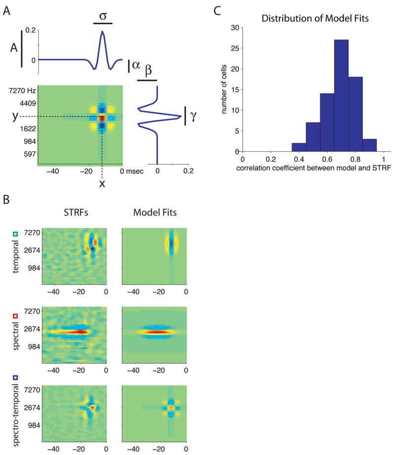
A) Schematic of the bivariate Mexican hat model and its parameters. A, overall scale; x, latency; y, best frequency; σ: temporal width; γ: spectral width; α: depth of temporal sidebands; β: depth of spectral sidebands. The sigma and gamma parameters capture the breadth of tuning in temporal or spectral domains, respectively. Alpha and beta describe each STRF’s sensitivity to temporal and spectral modulations.

B) Examples of model fits to real data. Left panels: STRFs shown as examples in previous figures. Right panels: STRFs generated by model fits to those examples.

C) Distribution of correlation coefficients between STRFs and model fits.

Figure 3B shows examples of fits of the model to the 3 example STRFs from figure 2. Qualitatively, the model is able to capture many aspects of each STRF, including its preferred frequency and latency, its widths in spectrum and time, and its selectivity for spectral features, temporal features, or both. Figure 3C shows the distribution of correlation coefficients between STRF and model for all cells (mean cc = 0.69 +/− 0.11 standard deviation). For comparison, the three examples shown had correlation coefficients of 0.72 (temporal), 0.88 (spectral), and 0.74 (spectro-temporal) respectively. Figure S3 shows the distribution of latencies, best frequencies, and spectral and temporal widths obtained from model fits to all cells, along with estimates of these parameters obtained by directly measuring the STRFs. The two distributions show good agreement.

Plotting the fitted spectral versus temporal widths for all cells revealed an L-shaped distribution (figure 4A). All but 2 cells were less than 0.6 octaves wide in spectrum and/or less than 7 msec wide in time. Qualitatively similar (though noisier) results were obtained by measuring the half-width of temporal and spectral cross-sections through the peak of each STRF (figure S4A). The locations of the example cells from figure 2 are given by green (temporal), red (spectral), and blue (spectro-temporal) circles, and represent the two arms and the hinge of the distribution. The distribution of cells along the two axes suggests that all STRFs are narrowly tuned in at least one dimension, while integrating over a range of different times and bandwidths in their other (non-tuned) dimension. There is a striking absence of cells that integrate broadly over both dimensions.

Figure 4. STRFs show a highly structured distribution of shapes.

A) Spectral width versus temporal width for all STRFs (n=71). Width parameters were obtained by fitting the bivariate Mexican hat model to each STRF. They show an L-shaped distribution, with most cells narrowly tuned in spectrum, time, or both. Example cells from figure 2 are indicated by green (temporal, example 2A), red (spectral, example 2B), and blue (spectro-temporal, example 2C) squares in this and the following figures.

B) Depth of spectral versus temporal sidebands for all STRFs. Depth parameters show an inverted L-shaped distribution, with all cells showing significant sidebands in at least one of the two dimensions.

C) Depth of temporal sidebands versus temporal width. Cells that are narrowly tuned in time show stronger temporal sidebands, while cells that are broadly tuned in time show weak temporal sidebands.

D) Depth of spectral sidebands versus spectral width. Cells that are narrowly tuned in spectrum generally show strong spectral sidebands. Cells that are broadly tuned in spectrum show more varied behavior.

E) Distribution of symmetry indices obtained from modulation spectra for each STRF. The asymmetry of the modulation spectrum reflects the degree to which a STRF is selective for oriented time-frequency sweeps. Most cells of all types show symmetry values near zero, indicating little orientation tuning.

F) Distribution of orientation parameters obtained by fitting a version of the bi-variate Mexican hat model including an orientation term. Most cells show orientations near zero, indicating that they are aligned largely along the temporal and /or spectral axes.

Related structure is evident in a plot of spectral versus temporal sideband depth (figure 4B). All cells showed prominent sidebands (alpha > 1, beta > 0.8) in at least one of the two dimensions, leading to an inverted L-shaped distribution. These data indicate that all cells were sensitive to modulations along at least one dimension. To ask whether cells tended to show sensitivity to modulations along their narrowly tuned dimension, we plotted the depth of temporal (or spectral) sidebands versus temporal (or spectral) width. As shown in figure 4C, strong temporal sidebands were associated with narrow temporal tuning (cc = −0.79, p = 3.5e-16). The relationship between strong spectral sidebands and narrow spectral tuning was weaker (figure 4D; cc = −0.21, p = 0.07), but this was largely due to three outliers with extremely high values of beta and wider spectral tuning. When these three outliers were omitted from the population, the correlation was −0.43, p=2.9e-4. Together these data indicate that nearly all STRFs showed narrow tuning and alternating sidebands along at least one dimension.

We observed very few STRFs showing strong orientation in time-frequency space, and hence selectivity for upward or downward frequency sweeps. We quantified orientation selectivity in two ways. First, we calculated the symmetry index (see Methods) of the two sides of each STRF’s modulation spectrum. Un-oriented STRFs have symmetry indices close to zero, while STRFs with strong orientation selectivity have symmetry indices approaching +1 or −1. As shown in figure 4E, most cells had symmetry indices near zero (std = 0.15), indicating that they were largely un-oriented. Second, since our original model could only produce STRFs oriented along the x and/or y axes, we fit the STRFs to a slightly more complex version of our model that included an orientation parameter (see Suppl. Methods). The distribution of orientations obtained from these fits (figure 4F) looks very similar to the distribution of symmetries (std = 8.5°), confirming that most cells in our population were closely aligned to the temporal and/or spectral axes, and validating our choice of the basic Mexican-hat model.

STRF dependence on stimulus intensity

In a previous study (Nagel and Doupe, 2006) we found that the temporal response properties of most field L neurons changed rapidly and systematically with stimulus intensity. To investigate the effects of intensity on receptive fields in both time and frequency, we compared STRFs from the same neurons, obtained with the same stimulus segments, played at 63 and 30dB. The intensity of the stimulus alternated continuously every 5 seconds for a total of 33 minutes, ensuring that intensity-driven changes in STRFs could not be due to long-term changes in the animal’s state. We found that STRFs in different regions of the shape distribution showed different types of intensity dependence.

STRFs that were narrowly tuned in both spectrum and time showed prominent changes in the depth of both spectral and temporal sidebands with sound intensity. A typical example is shown in figure 5 (additional examples in figure S1). At 30dB (figure 5A), the STRF has a single large positive peak flanked by shallow negative regions on all sides. At 63dB (figure 5B), the negative spectral sidebands are deeper and occur at a shorter latency; they are followed in time by small positive peaks. These differences can be seen more clearly in temporal and spectral cross-sections though both STRFs taken at the peak of the low intensity STRF (figures 5C and 5D). The negative sidebands in both cross-sections are deeper at 63dB (red) than at 30dB (blue). The temporal cross-section (figure 5C) also illustrates that the 63dB STRF is narrower and shifted forward in time relative to the 30dB STRF. Dashed lines in these two plots represent the standard deviation of five jackknife estimates of the STRF (see Supplementary Methods) and indicate that these differences are highly significant.

Figure 5. STRFs with different shapes show different changes with stimulus intensity.

A–D) STRFs measured from the same cell with two different stimulus intensities. (A) STRF at 30dB. (B) STRF at 63dB. The 63dB STRF has shorter latency, more prominent negative regions, and additional positive regions. (C) Temporal cross sections at 2.7 kHz through the 30dB (blue) and 63dB (red) STRFs. Dashed lines indicate the standard deviation from five jackknife estimates of the STRF. The 63dB STRF has a significantly shorter latency than the 30dB STRF. (D) Spectral cross sections at −12 msec through both STRFs, colored as above. Negative spectral sidebands are much more prominent in the 63dB STRF.

(E) Rasters (top two panels) and PSTHs (bottom panel) of the cell responding to same stimulus segment played at 30dB and at 63dB, illustrating the marked differences in output. Although the mean firing rate of the cell was slightly higher in response to the 63dB stimulus (104Hz at 63dB versus 76Hz at 30dB), the firing rate is modulated over the same range in both conditions (0–300Hz, bottom panel).

F) STRFs measured from a temporally-tuned cell at 30dB and and 63dB. Top left panel: 30dB STRF. Bottom left panel: 63dB STRF. Top right panel: temporal cross-sections through both STRFs at 3.0 kHz. Bottom right panel: spectral cross sections through both STRFs at −14 msec. This cell shows a dramatic change in temporal phase with stimulus intensity from one positive peak to two.

G) STRFs measured from a spectrally-tuned cell at 30dB and 63dB. Top left panel: 30dB STRF. Bottom left panel: 63dB STRF. Top right panel: temporal cross-sections through both STRFs at 1.8 kHz. Bottom right panel: spectral cross sections through both STRFs at −32 msec. The 63dB STRF (red) is slightly narrower in time than the 30dB STRF (blue). At 63dB the negative spectral regions of the STRF are slightly deeper, and a second positive peak has appeared at a higher frequency. The error bars on the estimates of spectral STRFs were generally much larger due to their low firing rates. The significance of changes in spectral STRFs is discussed in the text.

The consequences of these changes in STRF shape can be seen in response raster plots for the same stimulus at the two intensities (figure 5E). The cell responded robustly in both conditions, with peaks of equal magnitude, indicating that the differences between the two STRFs are not simply due to reduced spiking at 30B. In addition, although some peaks—such as the first two—occur in both responses, they occur at a shorter latency in response to the 63dB stimulus, while other peaks differ entirely between the two conditions. These data illustrate that subtle changes in the strength and relative latency of STRF peaks are associated with significant changes in the neural response to the same stimulus at different intensities.

Cells that were narrowly tuned in time but broadly tuned in frequency showed striking changes in temporal sensitivity, with inconsistent changes in the spectral domain. Many of these cells, such as the example in figure 5F, had a single positive peak at 30dB, but two significant positive peaks at 63dB, indicating a dramatic change in temporal phase. In contrast, changes in the spectral domain varied across these cells. This cell had slightly narrower spectral tuning at 63dB. However, other temporally-oriented cells became more broadly tuned at 63dB, or showed a shift in their preferred frequency.

Finally, cells with narrow spectral tuning, but wide temporal tuning, showed stronger spectral sidebands at 63 versus 30dB. In some cells, such as the example in figure 5G, additional spectral peaks also became more prominent at the higher intensity. Error bars on spectrally-tuned STRFs were often larger than those for other STRF types, because these cells fired many fewer spikes (see figure 7C). Intensity-dependent changes in these STRFs therefore appear less significant (figure 5G, right hand panels), although they are broadly similar to those observed in other STRFs (stronger negative regions and more positive peaks). To quantify a cell’s intensity dependence without relying on its STRF estimate, we calculated the correlation coefficient between its PSTHs in response to the same stimulus at 30and 63dB. If the cell responds to the same stimulus feature at both intensities, this correlation coefficient should be high. If not, it should be low. (Because the correlation coefficient compares the shape of two waveforms independent of their size, changes in PSTH magnitude will not affect the correlation). The average PSTH correlation for spectrally tuned cells (< =0.5 octaves, > 5 msec, cc = 0.30 +/− 0.19, std) was not significantly larger than that for spectro-temporally tuned cells (cc = 0.36 +/− 0.18) or for temporally tuned cells (cc = 0.25 +/−0.18), which both showed significant changes in STRF shape. These data suggest that all cell types respond to significantly different stimulus features at high and low stimulus intensities.

Figure 7. STRFs with different temporal response properties arise from cells with distinct physiology.

A) Panel 1: STRF with fast temporal response properties. Panels 2 and 3: raw voltage trace and narrow mean spike waveform of the cell that produced this STRF. Dashed lines in panel 3 indicate the standard deviation of the waveform. Panel 4: inter-spike interval (ISI) distribution for this cell, showing its short 1 msec refractory period.

B) Equivalent data for a STRF with slow temporal response properties. This cell had a wider spike and a longer relative refractory period.

C) Temporal width of STRF versus spontaneous firing rate for all single units that produced significant STRFs. Temporal width and spontaneous firing rate were significantly correlated (correlation coefficient = −0.55, p = 8.3e-7).

D) Temporal width of STRF versus spike width from trough to peak for all single units with significant STRFs. STRF and spike width were positively correlated (correlation coefficient = 0.72, p = 1.3e-12). Inset: schematic of spike width measurement. The width of the mean spike for each cell was measured from its trough to the subsequent peak.

Population Analysis of Intensity Effects

To quantify the intensity-dependent changes in STRF shape across our population, we fit the STRFs in each condition to the bi-variate Mexican hat model described above. Overall, this model fit STRFs obtained at 30dB as well as it did STRFs obtained at 63dB (mean correlation coefficient between model and STRF was 0.73+/−0.13 (std) at 30dB versus 0.69 +/−0.11 at 63dB).

The examples above suggest that STRFs show intensity-dependent changes in the magnitude of negative regions primarily along the dimensions for which they are narrowly tuned. To examine whether this held true at the population level, we divided our population into narrow- and broadly-tuned cells for each dimension (based on the temporal and spectral width parameters; figure 6A and E). We then plotted the values of alpha (reflecting temporal sideband depth) and beta (reflecting spectral sideband depth) for each of these subpopulations.

Figure 6. STRFs show intensity-dependent changes along the dimensions for which they are narrowly tuned.

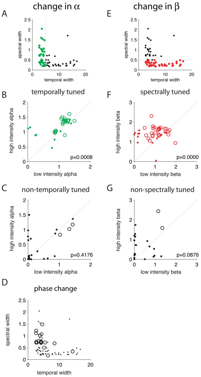
A–C) Intensity-dependent changes in the depth of temporal sidebands. (A) We divided our population into two groups depending on whether the spectral width was less than 5msec (green dots) or greater than 5 msec (black dots) at 63dB. (B) Value of the parameter alpha, reflecting temporal sideband depth, at 63dB versus 30dB for all cells with temporal widths less than 5msec (n=41). Cells showing significant changes are represented by open circles, while non-significant changes are represented by dots. 20 cells showed significant increases, while 2 showed significant decreases. Across this population, values of alpha were significantly higher at 63dB than at 30dB (p = 0.0008), indicating greater sensitivity to temporal modulations at the higher intensity. (C) Value of alpha at 63dB versus 30dB for cells with temporal widths greater than 5msec (n=30). As a whole, this population showed no consistent change in the magnitude of alpha (p=0.42). 3 cells showed significant decreases.

D) Spectral versus temporal width of cells showing phase change (sign inversion of the scaling term A from positive to negative), and of all cells (dots). Most cells that showed a phase change (circles) were narrowly tuned in time but broadly tuned in spectrum.

E–G) Intensity-dependent changes in the depth of spectral sidebands. (E) We divided our population into cells with spectral widths at 63dB less than 0.5 octaves (red dots) and greater than 0.5 octaves (black dots). (F) Value of the parameter beta, reflecting spectral sideband depth, at 63dB versus 30dB for all cells with spectral widths less than 0.5 octaves (n=45). 23 cells showed significant increases, while 4 showed significant decreases. Across this population, values of beta were significantly higher at 63dB than at 30dB (p = 1.9–5), indicating greater sensitivity to spectral modulations at the higher intensity. (G) Value of beta at 63dB versus 30dB for cells with temporal widths greater than 0.5 octaves (n=26). No consistent change in the magnitude of beta was observed (p=0.09). 2 cells showed significant increases.

Figure 6B shows the depth of temporal sidebands at 63 versus 30dB for STRFs that were narrowly tuned in time at 63dB (less than 5msec wide, green circles in figure 6A). Most points fall above the diagonal (p=0.0008, 20 cells with significant increases, 2 with significant decreases), indicating that in temporally-tuned cells, temporal sidebands generally become stronger at higher intensity. Figure 6C shows a similar plot for STRFs with temporal widths greater than 5msec. These cells show no systematic change in temporal sideband depth (p=0.42) and only 3 cells show significant changes in either direction. These effects were not strongly dependent on our particular classification of cells as temporally tuned: a similar difference between temporally-tuned and non-temporally-tuned cells was seen when we divided the populations at 4 msec or 6 msec.

Figure 6F shows the depth of spectral sidebands at 63 versus 30dB for STRFs that were narrowly tuned in spectrum at 63dB (less than 0.5 octaves wide). Again, most points fall above the diagonal (p=1.9e-5, 23 cells with significant increases, 4 with significant decreases), indicating that in spectrally-tuned cells, spectral sidebands are generally stronger at 63dB. In contrast, cells that are broadly tuned in spectrum show no consistent change in spectral sideband depth (figure 6G, p = 0.09). A similar difference between spectrally-tuned and non-spectrally-tuned cells was observed when we divided the two populations at 0.6 octaves.

Finally, to identify cells that showed a significant change in phase (number of positive peaks), we looked for cells whose scaling term (A) switched from from positive (one positive peak) at 30dB to negative (two positive peaks) at 63dB. Figure 6D shows cells with such a phase change (circles) overlaid on a plot of all cells’ spectral versus temporal width. The majority of cells with phase changes are narrowly tuned in time but broadly tuned in frequency.

Finally, while cells with different STRFs showed different patterns of sideband change, all STRFs tended to show narrower peaks in time at 63dB. This temporal narrowing can be seen in the spectrally-tuned example in figure 5G, and can be quantified by plotting the best temporal modulation frequency of each STRF at 63 versus 30dB (figure S4B). This generalized temporal narrowing is consistent with our previous finding (Nagel and Doupe, 2006) that most cells in field L show some temporal changes with stimulus intensity.

Together these data suggest that at high intensity, cells become more specialized for processing modulations, primarily along their preferred dimension

Physiological correlates of STRF characteristics

Cells with different STRFs differed systematically in their electrophysiological properties. Cells with STRFs that were narrowly tuned in time had high spontaneous firing rates and narrow spike waveforms, while cells with STRFs that integrated over longer time intervals had low spontaneous firing rates and wide spike waveforms. Figure 7A shows spike waveforms, and the distribution of inter-spike intervals (ISI), for a typical cell with narrow temporal tuning (temporal width = 3.7msec). It has a narrow spike, a short (1 msec) refractory period, and fired at high average rates both spontaneously (35 Hz) and when driven by our stimulus (104Hz). Figure 7B shows the same data for a cell with a STRF that is broad in time (temporal width = 9.8msec). Its spike has a much wider second peak, and the ISI histogram peaks at a longer latency. This cell fired at 6 Hz spontaneously, and at 10Hz on average when driven by the stimulus.

To examine whether these differences in firing rate and spike shape held at the population level, we plotted each cell’s spontaneous rate (figure 7C) and spike width (figure 7D) against its temporal width, obtained by fitting the bi-variate Mexican hat model as described above. Spontaneous firing rate was measured over the five seconds preceding the onset of the stimulus. Spike width was measured on the mean spike over the recording session (5900-374241 waveforms), from the first negative peak to the subsequent positive peak (see inset, figure 7D). We found a strong negative correlation between spontaneous firing rate and STRF temporal width (correlation coefficient = −0.55, p = 8.3e-7), and a strong positive correlation between spike width and temporal width correlation coefficient = 0.72, p = 1.3e-12). Similar strong correlations were found using the 50% width of a temporal cross section of each STRF, rather than the width obtained through fitting (cc for spontaneous firing rate and STRF width = −0.50, p = 6.6e-6; cc for spike width and STRF width = 0.67, p = 2.8e-11). We also verified that the correlations we observed were not due to differences in spike amplitude that might arise from variations in electrode placement (see Supplementary Analysis.)

Together, these data indicate that cells that are narrowly tuned in time have high firing rates and narrow spikes, while cells sensitive to slower modulations have lower firing rates and wider spikes. These data suggest that fast and slow responses arise from cells with distinct morphological or electrophysiological properties.

Anatomical distribution of STRF types

Field L is composed of several sub-regions (Fortune and Margoliash, 1992) defined by their anatomical location and different distributions of cell morphologies. L2 receives thalamic input and is reciprocally connected to the output areas L1 and L3. To examine whether different STRF types were localized to different regions of field L, we performed multi-unit mapping studies in 3 head-fixed birds sedated with diazepam. In each experiment, we advanced a four-electrode linear array in steps of 100 microns through the field L complex, and recorded single or multi-unit responses to our stimulus on all channels at each depth. After making marker lesions and perfusing, we prepared sagittal sections of each brain, and stained alternate sections with Nissl and with an antibody against the cannabinoid receptor CB1 that selectively labels the input area L2 (Soderstrom et al., 2004). Figure 8A shows one pair of such sections from one bird. Area L2 is a dark-staining area in the CB1 section, and a region of densely-packed cells surrounding the lighter-staining input fibers in the Nissl section (white arrows). The tracks of the four electrodes intersect L2 obliquely and are further identified by marker lesions.

Figure 8. STRFs with different temporal response properties are localized to different regions of field L.

A) Histological slides showing the regions of field L and the locations of electrode penetrations in a head-fixed mapping experiment. Top panel: slide stained with an antibody to CB1, the cannabinoid receptor, which selectively labels the input area L2 (white arrow). Above the stained area is area L1, below it is area L3. Tracks of four electrodes can be seen crossing the three layers of field L. Pink arrows indicate marker lesions. Bottom panel: Nissl-stained slide adjacent to above showing the lamina that define the borders of the field L complex, as well as the diagonal fiber tract immediately adjacent to field L2 (white arrow). Lesions on all four electrodes are visible.

B) Temporal best modulation frequency of raw multi-unit spike-triggered averages as a function of recording depth on each of four electrodes. Pink arrows mark the depths of the lesions shown in the top panel of (A). Sites with higher best modulation frequencies are found within a restricted range of depths that is deeper and narrower for the anterior electrodes and shallower and wider for the posterior electrodes. The location of these faster sites corresponds well to the location of the dark-staining area in the CB1 slide, suggesting that these faster sites are localized to area L2.

C–E) Temporal best modulation frequency of single and multi-unit sites as a function of recording depth for three additional experiments in two birds. Each axis represents one penetration with four electrodes; data from different electrodes are plotted on the same graph. Data from different electrodes have been aligned so that zero marks the center of the field L2, as defined anatomically. In each experiment, cells with higher best modulation frequencies are found only at the center, surrounding L2. Blue dots represent STAs recorded with the same stimulus used in chronic experiments. Gray dots represent STAs recorded with a more slowly-varying stimulus (see Suppl Methods). Data shown for each experiment were obtained with a single stimulus. The localization of faster responses to L2 can be seen with either stimulus.

F) Examples of raw spike-triggered averages (STAs) recorded at different depths show good spectral and temporal tuning.

To examine the temporal tuning of multi-electrode sites, we calculated the temporal best modulation frequency (temporal BMF, see Methods) of spike-triggered averages (STAs) obtained from sorted single- or multi-unit activity at each site. We used best modulation frequency rather than temporal width because it could be calculated directly from raw STAs without fitting. Figure 8B shows temporal BMF as a function of recording location in a single experiment. Recording sites with high temporal BMFs (narrow temporal tuning) were constrained to a narrow region of each penetration, that—like area L2—traverses the penetration field from ventro-rostral to dorso-caudal, and is more diffuse on the posterior side. Pink arrows show the depths of the marker lesions and support the localization of faster cells to area L2. Recording sites with low temporal BMFs (broad temporal tuning) were found throughout the penetration but were more common above and below the region of fast cells.

Localization of cells with fast response properties to L2 was seen in three additional mapping sessions from two birds. Figure 8C shows temporal BMF as a function of distance from the CB1-defined center of L2 in each of the three experiments. Data from 3–4 electrodes are plotted on each axis, and aligned so that zero represents the center of L2. STAs with higher temporal BMFs are concentrated near L2, while those sensitive to lower temporal frequencies are located above and below it. Examples of raw spike-triggered averages obtained in the last mapping experiment are shown at the far right. They illustrate that robust spectral and temporal tuning could be observed using multi-unit recording without decorrelation. Data from the chronically recorded birds show a similar localization pattern, with narrow-spiking cells sensitive to fast modulations generally concentrated in one region of the penetration (figure S5).

Discussion

Distribution of STRF Types

We observed a highly structured distribution of STRF shapes along two perpendicular axes. At moderately high stimulus intensities (63dB), STRFs were generally narrowly tuned along either the spectral or temporal axes or both, and showed alternating positive and negative bands along the dimensions for which they were narrowly tuned. Strongly oriented sweep-selective cells, and broadly tuned cells that would act as overall sound level detectors, were largely absent from our population. This distribution of response properties may be related to the structure of many natural sounds—including both zebra finch song and speech—which are dominated by pure temporal and pure spectral features, and contain comparatively few strongly oriented spectro-temporal sweeps (Singh and Theunissen, 2002, Woolley et al, 2005).

While our data agree broadly with previous studies of the distribution of STRF types in field L or mammalian auditory cortex, they differ in several important respects. Woolley et al. (2005) calculated the average modulation spectrum across field L neurons, and compared this ensemble modulation spectrum to the distribution of energy found in song. They concluded that field L is sensitive to a range of higher temporal frequencies but only to the lowest spectral frequencies. By looking at the distribution of individual cell types, rather than aggregate measures, we found instead that separate populations of temporal and spectral cells are tuned to higher-frequency modulations in each of these domains, while a third population is tuned to high frequency modulations in both domains. As in our study, Miller et al. (2002) found that most neurons in anesthetized cat A1 have fairly symmetric modulation spectra, indicating that they are not selective for oriented frequency sweeps. However, that study found no systematic relationship between the spectral and temporal tuning properties of A1 neurons, while we found a strong trade-off between temporal and spectral selectivity. These differences may arise from the structure of the avian forebrain, which contains many fast-firing cells able to follow rapid modulations in the stimulus, while the mammalian auditory cortex responds more slowly (Miller et al., 2002, Depireux et al., 2001, Lu et al., 2001). They may also arise from differences in recording conditions. Most previous studies have measured STRFs under pentobarbital anesthesia, while we recorded from unanesthetized animals. Anesthesia can profoundly influence the temporal dynamics of cortical auditory responses (Wang et al., 2005). Chi and Shamma (2005) have modeled A1 with receptive fields that evenly span a range of time-frequency orientations, similar to the uniform sampling of two-dimensional spatial orientations in visual cortex. However, the same group reported that A1 neurons show mostly symmetric tuning properties (Depireux et al., 2000; Simon et al., 2007). Together with data from these studies, our findings suggest that sampling of a range of temporal and spectral modulations, not orientation in time-frequency space, may be the organizing principle of forebrain auditory sensitivity.

STRF dependence on intensity

In a previous study (Nagel and Doupe, 2006), we found that the temporal receptive fields of field L neurons changed systematically with increases in the mean stimulus amplitude. At low intensities, receptive fields were mostly positive, indicating that cells responded whenever the stimulus amplitude was high, and thus acted as ‘integrators’ of sound over time. At higher mean intensities, the negative parts of the receptive fields grew larger and decreased in latency, causing the cells to behave as ‘differentiators’ rather than integrators, and to respond more selectively to amplitude changes. These receptive fields changes occurred rapidly after the stimulus mean increased or decreased, suggesting that they stemmed from nonlinearities in the neural response rather than time-dependent adaptations. Following arguments made for the visual system (Attick, 1992), we argued that such changes could be adaptive, allowing cells to become selective for particular temporal modulations when signal-to-noise levels were high, and to behave more like detectors when signal quality was low. Similar nonlinearities have been described in retinal ganglion cells, which respond to differences in local light intensity in bright light, but integrate over larger spatial regions at low luminance (Enroth-Cugell and Lennie, 1975). The results of the current study extend these findings to the time-frequency domain, suggesting that negative regions perpendicular to each STRFs’ dimension of narrow tuning grow stronger at high intensity, leading the population to separately analyze temporal and spectral structure in the stimulus. At low intensities, in contrast, all cells behave more like low-pass detectors (figure 9A).

Figure 9. A model of STRF dependence on intensity.

A) Schematic summary of auditory encoding in field L across intensities. At low stimulus intensities (gray region), STRFs are dominated by large positive regions that can be elongated in time or frequency. These STRFs behave as “detectors” responding whenever there is sound energy present within the receptive field. At high stimulus intensities (white region), negative regions oriented in time, spectrum, or both, appear. These ensure that cells only respond when the energy in the positive region of the STRF is greater than that at nearby frequencies or times, making cells more selective for differences or changes in their preferred dimension.

B) A simple biophysical model can account for the dependence of STRFs on stimulus intensity. In this model, the cell we are recording from (or some cell upstream from it; shown in black) receives at least two inputs, one excitatory (red) and one inhibitory (blue).

C) In this model, the response properties of the output neuron (black) can be modeled as the sum of the nonlinear responses of its excitatory (red) and inhibitory (blue) inputs. The response of each input neuron is calculated by convolving its receptive field (first column) with the stimulus, summing, then nonlinearly transforming the output of the receptive fields according to a nonlinear gain function (second column). The STRF measured for the output neuron will reflect a weighted sum of the two input receptive fields. Each receptive field is weighted by the slope of its gain function in the region explored by the stimulus. Because stimuli with different mean intensities explore different regions of the gain function (vertical lines), the STRF will reflect different combinations of excitatory and inhibitory inputs at 30 and 63dB.

Although these results agree broadly with our previous study, one difference is notable. In that paper, we found that all cells—taken as a population—show changes both in preferred temporal frequency and in the balance of positive and negative components in the temporal domain. In this study, we likewise found that most cells have somewhat narrower peaks at 63 versus 30dB, reflected in an increase in best temporal modulation frequency at high stimulus intensities. However, here cells only show consistent changes in the magnitude of negative sidebands along their narrowly tuned axes. We believe this difference arises from two factors. First, the temporal receptive fields of the previous paper represent spectral averages of the true STRF of the cell. Because spectral peaks and sidebands have different temporal extents, changes in their magnitude can appear, in averages across spectrum, to be changes in “temporal” differentiation. Second, in our previous paper we analyzed the behavior of all recorded cells together, and did not divide our population into separate groups. When considered as a single population, the cells recorded in the current study also show significant changes in both temporal and spectral differentiation, because around two-thirds of the population is tuned in each domain, and the remaining cells generally show inconsistent changes. The ability to visualize tuning in both the spectral and temporal domains, combined with the greater number of cells recorded in the present study, allowed us to identify differences between populations within field L that we were unable to resolve in the previous study.

These data suggest a simple model (figure 9B and 9C) in which excitatory and inhibitory inputs interact systematically to give rise to the intensity-dependent receptive fields we recorded. In this model, the cell we are recording from (or some cell afferent to it) receives input from at least two cells, one excitatory and one inhibitory. The response of each input cell is modeled as a linear receptive field—like the STRFs measured in this study—followed by a nonlinear gain function. This gain function mimics the effects of a spiking threshold and saturation on the cell’s output; its slope determines how strongly the cell fires when driven by appropriate stimuli. Different stimulus intensities will explore different regions of the nonlinearity, producing different average gains. As the intensity of the stimulus increases, the latency of the inhibitory input decreases, while its gain increases relative to that of the excitatory input. Because the output cell receives a different balance of excitatory and inhibitory inputs at 30 and at 63dB, its STRFs at these two intensities will reflect different combinations of the excitatory and inhibitory neurons’ receptive fields. Such circuitry could be present in the forebrain or cortex (Wehr and Zador, 2003; Tan and Schreiner, 2004), or could shape responses of more peripheral neurons that pass their response properties on to higher areas (Nelken and Young, 1994; Yu and Young, 2000). A non-linear encoding model like the one we describe would more accurately capture the response properties of field L neurons, but would also raise difficulties for existing models of how acoustic stimulus identity is decoded (Drew and Abbott, 2003, Chi and Shamma, 2005).

Correlations with Physiology and Anatomy

Finally, we found that cells with different temporal response properties also differ in their physiology and anatomical distribution. Cells tuned to fast temporal frequencies had high spontaneous and driven rates, fired spikes with narrow waveforms, and were located in a restricted region of each penetration. Our multi-unit mapping study indicated that this restricted region corresponds to the input layer L2, in agreement with a previous study showing higher average best modulation frequencies in L2 (Sen et al., 2001). Cells that integrated over longer time intervals were found throughout the penetration, but were more prevalent in the output regions L1 and L3. These cells had much lower spontaneous and driven rates, longer latencies, and fired wider spikes. These data suggest that fast and slow response types may arise from cells with different morphological or electrical properties, concentrated in different anatomical regions.

Biophysically, narrow spikes and high firing rates can arise from small or electrotonically compact cells that can repolarize quickly and track rapid fluctuations in their synaptic input. Such cells may have specialized potassium channels that give them faster kinetics (Martina et al., 1997, 1998; Chow et al., 1999). Conversely, a large or electrotonically extended cell will have a wider spike and longer refractory period, leading to lower firing rates, and more low-pass filtering of its input. The subregions of field L have been shown to differ in their distribution of cell sizes and morphologies (Fortune and Margoliash, 1992): L2 contains more small and medium bodied cells with compact dendritic fields. L1 and L3 have more large- and medium-bodied cells with extensive dendritic fields. We therefore hypothesize that fast temporal responses may arise from smaller cells with more compact dendrites, while slow temporal responses may arise from larger cells with dendritic conductances that allow them to integrate inputs over time.

In the mammalian hippocampus and cortex, narrow extracellular spike waveforms have been linked to inhibitory interneurons (Buzsaki and Eidelberg 1982, Henze et al, 2000), which have narrower spike waveforms in intracellular recordings (Buhl et al. 1996). About 30–40% of neurons in the auditory forebrain are estimated to be GABAergic (Pinaud et al, 2004, 2007), but physiological differences between inhibitory and excitatory cells in these areas have not been explored. Due to the density of units with fast responses and narrow spikes in regions of our penetration, we think it is unlikely that fast responses arise exclusively from inhibitory neurons, although this remains an open possibility.

Our data fit with previous studies showing that auditory neurons become tuned for progressively slower temporal modulations at successive levels of the auditory hierarchy (Creutzfeldt, O. 1980; Sen et al, 2001; Miller et al, 2002; Linden et al, 2003). In contrast to mammalian systems, where a large difference in temporal following is seen between inferior colliculus and cortex (Langer and Schreiner, 1988, Miller et al, 2002), but not between successive cortical stages, we see a sharp distinction between the input and output layers of the avian primary auditory area. This may indicate that L2 shares more properties with the mammalian inferior colliculus, as suggested by Las et al (2005). It may also indicate substantial differences in the range of temporal frequencies processed by avian and mammalian forebrain auditory areas.

In the auditory brainstem of both mammals and birds, distinct temporal response patterns have been linked to the distinct morphologies and electrical properties of bushy and stellate cells (Rhode and Smith, 1983, 1986, Sullivan, 1985, Oertel, 1991). These different response properties are in turn related to different functional roles in encoding phase and intensity information (Sullivan, 1985; Takahashi et al, 1984). Although intracellular recordings and labeling experiments will be required to definitively link cellular properties to auditory responses in field L, our data suggest that similar relationships between structure and function exist for auditory neurons in the avian forebrain.

Methods

Chronic Electrophysiology

We used chronically implanted microdrives (Hessler and Doupe, 1999) with 2–3 tungsten electrodes (MicroProbe Inc, Gaithersburg, MD) to record single units (n = 81) from 5 adult male zebra finches. A detailed description of microdrive construction and implantation are given in that paper.

Chronic recording procedures and stimulus presentation methods were similar to those described in Nagel and Doupe (2006), except that a commercial spike sorter (Plexon Offline Sorter, Plexon, Dallas, TX) was used in addition to custom software (Matlab). Spikes were sorted based on the similarity of overlaid spike waveforms and on clustering of waveform projections in a two-dimensional principal component space, and were considered isolated if they contained fewer than one violation of 1 msec refractoriness per thousand spikes.

During recording, the chamber lights were kept off to minimize movement and birds were monitored only with an infrared camera. We therefore state that they were “unanaesthetized,” not that they were awake.

Acute Electrophysiology

We performed acute mapping experiments in three additional adult male birds. A few days prior to the experiment, we prepared the bird for acute physiology under brief equithesin (3.5μl/g, Hessler and Doupe, 1999) anesthesia by making an opening through the skull over the location of field L, affixing a stereotaxic metal pin to the skull with dental cement, and covering the skull opening was covered with a silicone elastomer (World Precision Instruments).

On the day of the experiment, the bird was sedated with diazapam (30μl) and placed in a stereotaxic device. We removed the silicone covering, advanced a linear array of four electrodes into the brain in 100 micron steps, and recorded activity on all channels if auditory activity was observed on any channel. Single and multi-unit activity was sorted using the Plexon offline sorter. Multi-unit clusters were separated into multiple clusters if this increased the signal quality of the STRFs produced from each cluster.

After the final recordings, we made electrolytic lesions at several depths along the electrode penetrations. Birds were lethally anesthetized and perfused with saline and 4% paraformaldehyde. To identify the location of recording sites, alternate 40 micron brain sections were Nissl-stained or labeled for CB1, a marker for the input region L2 (Soderstrom et al., 2004),

Stimulus

The stimulus was composed of 30 or 32 logarithmically spaced narrowband noise signals, each created by passing a white noise signal through a filter that was Gaussian in log frequency (Figure 1A). The center frequencies of the filters cf_n were given by

$$c{f}_n=exp(log(400)+0.1(n-1))$$

where cf_n is the center frequency of the nth band. Filters overlapped by one standard deviation so that the summed narrowband noises had close to a flat envelope (Theunissen et al, 1998). Each narrowband signal was modulated by a different envelope (Figure 2B). Envelopes were produced by smoothing white noise with an exponential filter, so that the log envelope (envelope in dB) had an exponential power spectrum

$$P(f)=exp(-f/50\text{Hz})$$

where P is the power in the log envelope and f is frequency. These envelopes were statistically identical to those used in a previous experiment (Nagel and Doupe, 2006). For a subset of the acute mapping experiments we used a more slowly varying set of log envelopes (see Suppl. Methods and Figure S6).

By adjusting the mean of the log envelopes, we manipulated the intensity of our stimulus: two conditions, 63dB mean, 6dB standard deviation, and 30dB mean, 6dB standard deviation, alternated smoothly every five seconds. Half of our stimulus was composed of repeats of the same stimulus segment while the remainder were unique segments. Unique segments were used to estimate the STRF and nonlinearity for each neuron, while predictions were tested on the repeated segments.

STRF estimation

STRFs were estimated by cross-correlating the spike train with each row of the spectrogram, yielding the spike-triggered average (STA), then “decorrelating” the STA to remove the influence of stimulus correlations. This procedure is broadly similar to that described in Theunissen et al., (2000) and is described in detail in supplementary methods.

Modulation Spectra and STRF measurements

Modulation spectra of STRFs were obtained by taking the two dimensional Fourier transform of the two dimensional autocorrelation function of the STRF (Singh and Theunissen, 2003). We calculated a symmetry index (Miller et al, 2002) by dividing the modulation spectrum into left and right halves (M_left and M_right, respectively), then computing:

$$\frac{\mathrm{\sum }{M}_{\mathit{right}}-\mathrm{\sum }{M}_{\mathit{left}}}{\mathrm{\sum }{M}_{\mathit{right}}+\mathrm{\sum }{M}_{\mathit{left}}}$$

This index ranges from −1 to 1, and is zero for perfectly symmetric STRFs. The temporal best modulation frequency (BMF) of a STRF was obtained by folding the spectrum about its y-axis, averaging this folded spectrum across spectral frequencies, and finding the location of its maximum.

The latency and best frequency of each STRF were defined as the time and frequency of the STRF maximum. The 50% width and bandwidth were defined as the interval over cross-sections through the best frequency and latency that had an amplitude greater than or equal to half the maximum amplitude.

To quantitatively describe the distribution of STRF shapes, and the change in these shapes with stimulus intensity, we fit each STRF under each stimulus condition to a bi-variate Mexican hat model:

$$\begin{array}{l}{x}^{\prime }=x-\mu \\ y^{\prime }=y-\nu \\ G(x,y)=A{e}^{-{\sigma }^2{x^{\prime }}^2-{\gamma }^2-{y^{\prime }}^2}(1-{\alpha }^2{\sigma }^2{x^{\prime }}^2)(1-{\beta }^2{\gamma }^2{y^{\prime }}^2)\end{array}$$

where A is the magnitude and sign of the filter; μ, the latency; ν, the center frequency; σ, the temporal width; γ, the spectral width; α, the depth of temporal sidebands, and β, the depth of spectral sidebands. Details of the fitting procedure are described in Suppl Methods.

Nonlinearities and Predictions

The nonlinear relationship between each STRF’s output and the cell’s actual response was calculated following the method of Brenner et al (2001). Predicted responses to repeated stimulus segments were made by first convolving the STRF with the spectrogram of this repeated segment, summing across bands, then applying the nonlinearity to the output of this convolution. The first 500 milliseconds of both the predicted and actual PSTH were omitted from the comparison because this often contained a slowly adapting component not predicted by the STRF model. Correlation coefficients between actual and predicted STRFs for the remaining 4.5 seconds are shown in figure S2A.

References

- Atick JJ. Could Information-Theory Provide an Ecological Theory of Sensory Processing. Network-Computation in Neural Systems. 1992;3:213–251. doi: 10.3109/0954898X.2011.638888. [DOI] [PubMed] [Google Scholar]
- Barbour DL, Wang X. Auditory cortical responses elicited in awake primates by random spectrum stimuli. J Neurosci. 2003;23:7194–206. doi: 10.1523/JNEUROSCI.23-18-07194.2003. [DOI] [PMC free article] [PubMed] [Google Scholar]
- Brenner N, Bialek W, de Ruyter van Steveninck R. Adaptive rescaling maximizes information transmission. Neuron. 2000;26:695–702. doi: 10.1016/s0896-6273(00)81205-2. [DOI] [PubMed] [Google Scholar]
- Buhl EH, Szilagyi T, Halasi K, Somogyi P. Physiological properties of anatomically identified basket and bistratified cells in the CA1 area of the rat hippocampus in vitro. Hippocampus. 1996;6:294–305. doi: 10.1002/(SICI)1098-1063(1996)6:3<294::AID-HIPO7>3.0.CO;2-N. [DOI] [PubMed] [Google Scholar]
- Buzsaki G, Eidelberg E. Direct afferent excitation and long-term potentiation of hippocampal interneurons. J Neurophysiol. 1982;48:597–607. doi: 10.1152/jn.1982.48.3.597. [DOI] [PubMed] [Google Scholar]
- Cheung SW, Nagarajan SS, Bedenbaugh PH, Schreiner CE, Wang X, Wong A. Auditory cortical neuron response differences under isoflurane versus pentobarbital anesthesia. Hear Res. 2001;156:115–27. doi: 10.1016/s0378-5955(01)00272-6. [DOI] [PubMed] [Google Scholar]
- Chi T, Ru P, Shamma SA. Multiresolution spectrotemporal analysis of complex sounds. J Acoust Soc Am. 2005;118:887–906. doi: 10.1121/1.1945807. [DOI] [PubMed] [Google Scholar]
- Chow A, Erisir A, Farb C, Nadal MS, Ozaita A, Lau D, Welker E, Rudy B. K(+) channel expression distinguishes subpopulations of parvalbumin- and somatostatin-containing neocortical interneurons. J Neurosci. 1999;19:9332–45. doi: 10.1523/JNEUROSCI.19-21-09332.1999. [DOI] [PMC free article] [PubMed] [Google Scholar]
- Creutzfeldt O, Hellweg FC, Schreiner CE. Thalamocortical transformation of responses to complex auditory stimuli. Exp Brain Res. 1980;39:87–104. doi: 10.1007/BF00237072. [DOI] [PubMed] [Google Scholar]
- Depireux DA, Simon JZ, Klein DJ, Shamma SA. Spectro-temporal response field characterization with dynamic ripples in ferret primary auditory cortex. J Neurophysiol. 2001;85:1220–34. doi: 10.1152/jn.2001.85.3.1220. [DOI] [PubMed] [Google Scholar]
- Drew PJ, Abbott LF. Model of song selectivity and sequence generation in area HVc of the songbird. J Neurophysiol. 2003;89:2697–706. doi: 10.1152/jn.00801.2002. [DOI] [PubMed] [Google Scholar]
- Eggermont JJ, Johannesma PM, Aertsen AM. Reverse-correlation methods in auditory research. Q Rev Biophys. 1983;16:341–414. doi: 10.1017/s0033583500005126. [DOI] [PubMed] [Google Scholar]
- Enroth-Cugell C, Lennie P. The control of retinal ganglion cell discharge by receptive field surrounds. J Physiol. 1975;247:551–78. doi: 10.1113/jphysiol.1975.sp010947. [DOI] [PMC free article] [PubMed] [Google Scholar]
- Escabi MA, Miller LM, Read HL, Schriner CE. Naturalistic auditory contrast improves spectrotemporal coding in the cat inferior colliculus. J Neurosci. 2003;23:11489–504. doi: 10.1523/JNEUROSCI.23-37-11489.2003. [DOI] [PMC free article] [PubMed] [Google Scholar]
- Fortune ES, Margoliash D. Cytoarchitectonic organization and morphology of cells of the field L complex in male zebra finches (Taenopygia guttata) J Comp Neurol. 1992;325:388–404. doi: 10.1002/cne.903250306. [DOI] [PubMed] [Google Scholar]
- Fortune ES, Margoliash D. Parallel pathways and convergence onto HVc and adjacent neostriatum of adult zebra finches (Taeniopygia guttata) J Comp Neurol. 1995;360:413–41. doi: 10.1002/cne.903600305. [DOI] [PubMed] [Google Scholar]
- Frisina RD. Subcortical neural coding mechanisms for auditory temporal processing. Hear Res. 2001;158:1–27. doi: 10.1016/s0378-5955(01)00296-9. [DOI] [PubMed] [Google Scholar]
- Gehr DD, Capsius B, Grabner P, Gahr M, Leppelsack HJ. Functional organisation of the field-L-complex of adult male zebra finches. Neuroreport. 1999;10:375–80. doi: 10.1097/00001756-199902050-00030. [DOI] [PubMed] [Google Scholar]
- Gentner TQ, Margoliash D. Neuronal populations and single cells representing learned auditory objects. Nature. 2003;424:669–74. doi: 10.1038/nature01731. [DOI] [PMC free article] [PubMed] [Google Scholar]
- Gill P, Zhang J, et al. J Comput Neurosci. Vol. 21. 2006. Sound representation methods for spectro-temporal receptive field estimation; pp. 5–20. [DOI] [PubMed] [Google Scholar]
- Heil P, Scheich H. Quantitative analysis and two-dimensional reconstruction of the tonotopic organization of the auditory field L in the chick from 2-deoxyglucose data. Exp Brain Res. 1985;58:532–43. doi: 10.1007/BF00235869. [DOI] [PubMed] [Google Scholar]
- Henze DA, Borhegyi Z, Borhegyi Z, Csicsvari J, Mamiya A, Harris KD, Buzsaki G. Intracellular features predicted by extracellular recordings in the hippocampus in vivo. J Neurophysiol. 2000;84:390–400. doi: 10.1152/jn.2000.84.1.390. [DOI] [PubMed] [Google Scholar]
- Hessler NA, Doupe AJ. Singing-related neural activity in a dorsal forebrain-basal ganglia circuit of adult zebra finches. J Neurosci. 1999;19:10461–81. doi: 10.1523/JNEUROSCI.19-23-10461.1999. [DOI] [PMC free article] [PubMed] [Google Scholar]
- Hubel DH, Wiesel TN. Receptive fields, binocular interaction and functional architecture in the cat’s visual cortex. J Physiol. 1962;160:106–54. doi: 10.1113/jphysiol.1962.sp006837. [DOI] [PMC free article] [PubMed] [Google Scholar]
- Kowalski N, Depireux DA, Shamma SA. Analysis of dynamic spectra in ferret primary auditory cortex. II. Prediction of unit responses to arbitrary dynamic spectra. J Neurophysiol. 1996;76:3524–34. doi: 10.1152/jn.1996.76.5.3524. [DOI] [PubMed] [Google Scholar]
- Kowalski N, Depireux DA, Shamma SA. Analysis of dynamic spectra in ferret primary auditory cortex. I. Characteristics of single-unit responses to moving ripple spectra. J Neurophysiol. 1996;76:3503–23. doi: 10.1152/jn.1996.76.5.3503. [DOI] [PubMed] [Google Scholar]
- Lewicki MS, Arthur BJ. Hierarchical organization of auditory temporal context sensitivity. J Neurosci. 1996;16:6987–98. doi: 10.1523/JNEUROSCI.16-21-06987.1996. [DOI] [PMC free article] [PubMed] [Google Scholar]
- Liang L, Lu T, Wang X. Neural representations of sinusoidal amplitude and frequency modulations in the primary auditory cortex of awake primates. J Neurophysiol. 2002;87:2237–61. doi: 10.1152/jn.2002.87.5.2237. [DOI] [PubMed] [Google Scholar]
- Linden JF, Liu RC, Sahani M, Schreiner CE, Merzenich MM. Spectrotemporal structure of receptive fields in areas AI and AAF of mouse auditory cortex. J Neurophysiol. 2003;90:2660–75. doi: 10.1152/jn.00751.2002. [DOI] [PubMed] [Google Scholar]
- Lu T, Liang L, Wang X. Temporal and rate representations of time-varying signals in the auditory cortex of awake primates. Nat Neurosci. 2001;4:1131–8. doi: 10.1038/nn737. [DOI] [PubMed] [Google Scholar]
- Machens CK, Wehr MS, Zador AM. Linearity of cortical receptive fields measured with natural sounds. J Neurosci. 2004;24:1089–100. doi: 10.1523/JNEUROSCI.4445-03.2004. [DOI] [PMC free article] [PubMed] [Google Scholar]
- Martina M, Schultz JH, Ehmke H, Moyner H, Jonas P. Functional and molecular differences between voltage-gated K+ channels of fast-spiking interneurons and pyramidal neurons of rat hippocampus. J Neurosci. 1998;18:8111–25. doi: 10.1523/JNEUROSCI.18-20-08111.1998. [DOI] [PMC free article] [PubMed] [Google Scholar]
- Miller LM, Escabi MA, Read HL, Schreiner CE. Spectrotemporal receptive fields in the lemniscal auditory thalamus and cortex. J Neurophysiol. 2002;87:516–27. doi: 10.1152/jn.00395.2001. [DOI] [PubMed] [Google Scholar]
- Muller CM, Leppelsack HJ. Feature extraction and tonotopic organization in the avian auditory forebrain. Exp Brain Res. 1985;59:587–99. doi: 10.1007/BF00261351. [DOI] [PubMed] [Google Scholar]
- Nagel KI, Doupe AJ. Temporal processing and adaptation in the songbird auditory forebrain. Neuron. 2006;51:845–59. doi: 10.1016/j.neuron.2006.08.030. [DOI] [PubMed] [Google Scholar]
- Nelken I, Young ED. Two separate inhibitory mechanisms shape the responses of dorsal cochlear nucleus type IV units to narrowband and wideband stimuli. J Neurophysiol. 1994;71:2446–62. doi: 10.1152/jn.1994.71.6.2446. [DOI] [PubMed] [Google Scholar]
- Oertel D. The role of intrinsic neuronal properties in the encoding of auditory information in the cochlear nuclei. Curr Opin Neurobiol. 1991;1:221–8. doi: 10.1016/0959-4388(91)90082-i. [DOI] [PubMed] [Google Scholar]
- Phillips DP, Irvine DR. Responses of single neurons in physiologically defined primary auditory cortex (AI) of the cat: frequency tuning and responses to intensity. J Neurophysiol. 1981;45(1):48–58. doi: 10.1152/jn.1981.45.1.48. [DOI] [PubMed] [Google Scholar]
- Phillips DP, Hall SE. Responses of single neurons in cat auditory cortex to time-varying stimuli: linear amplitude modulations. Exp Brain Res. 1987;67:479–92. doi: 10.1007/BF00247281. [DOI] [PubMed] [Google Scholar]
- Pinaud R, Velho TA, Jeong JK, Tremere LA, Leao RM, von Gersdorff H, Mello CV. GABAergic neurons participate in the brain’s response to birdsong auditory stimulation. Eur J Neurosci. 2004;20:1318–30. doi: 10.1111/j.1460-9568.2004.03585.x. [DOI] [PubMed] [Google Scholar]
- Pinaud R, Mello CV. GABA immunoreactivity in auditory and song control brain areas of zebra finches. J Chem Neuroanat. 2007;34:1–21. doi: 10.1016/j.jchemneu.2007.03.005. [DOI] [PMC free article] [PubMed] [Google Scholar]
- Qiu A, Schreiner CE, et al. Gabor analysis of auditory midbrain receptive fields: spectro-temporal and binaural composition. J Neurophysiol. 2003;90:456–76. doi: 10.1152/jn.00851.2002. [DOI] [PubMed] [Google Scholar]
- Rhode WS, Smith PH, Oertel D. Physiological response properties of cells labeled intracellularly with horseradish peroxidase in cat dorsal cochlear nucleus. J Comp Neurol. 1983;213:426–47. doi: 10.1002/cne.902130407. [DOI] [PubMed] [Google Scholar]
- Rhode WS, Smith PH. Encoding timing and intensity in the ventral cochlear nucleus of the cat. J Neurophysiol. 1986;56:261–86. doi: 10.1152/jn.1986.56.2.261. [DOI] [PubMed] [Google Scholar]
- Ringach DL, Hawken MJ, Shapley R. Receptive field structure of neurons in monkey primary visual cortex revealed by stimulation with natural image sequences. J Vis. 2002;2:12–24. doi: 10.1167/2.1.2. [DOI] [PubMed] [Google Scholar]
- Scheich H, Bonke BA, Bonke D, Langner G. Functional organization of some auditory nuclei in the guinea fowl demonstrated by the 2-deoxyglucose technique. Cell Tissue Res. 1979;204:17–27. doi: 10.1007/BF00235161. [DOI] [PubMed] [Google Scholar]
- Schreiner CE, Sutter ML. Topography of excitatory bandwidth in cat primary auditory cortex: single-neuron versus multiple-neuron recordings. J Neurophysiol. 1992;68:1487–502. doi: 10.1152/jn.1992.68.5.1487. [DOI] [PubMed] [Google Scholar]
- Schreiner CE, Mendelson J, Raggio MW, Brosch M, Kruegger K. Temporal processing in cat primary auditory cortex. Acta Otolaryngol Suppl. 1997;532:54–60. doi: 10.3109/00016489709126145. [DOI] [PubMed] [Google Scholar]
- Sen K, Theunissen FE, Doupe AJ. Feature analysis of natural sounds in the songbird auditory forebrain. J Neurophysiol. 2001;86:1445–58. doi: 10.1152/jn.2001.86.3.1445. [DOI] [PubMed] [Google Scholar]
- Sharpee TO, Sugihara H, Kurgansky AV, Rebrik SP, Stryker MP, Miller KD. Adaptive filtering enhances information transmission in visual cortex. Nature. 2006;439:936–42. doi: 10.1038/nature04519. [DOI] [PMC free article] [PubMed] [Google Scholar]
- Singh NC, Theunissen FE. Modulation spectra of natural sounds and ethological theories of auditory processing. J Acoust Soc Am. 2003;114:3394–411. doi: 10.1121/1.1624067. [DOI] [PubMed] [Google Scholar]
- Soderstrom K, Tian Q, Valenti M, Di Marzo V. Endocannabinoids link feeding stats and auditory perception-related gene expression. J Neurosci. 2004;24:10013–21. doi: 10.1523/JNEUROSCI.3298-04.2004. [DOI] [PMC free article] [PubMed] [Google Scholar]
- Sullivan WE. Classification of response patterns in cochlear nucleus of barn owl: correlation with functional response properties. J Neurophysiol. 1985;53:201–16. doi: 10.1152/jn.1985.53.1.201. [DOI] [PubMed] [Google Scholar]
- Takahashi T, Moiseff A, Konishi M. Time and intensity cues are processed independently in the auditory system of the owl. J Neurosci. 1984;4:1781–6. doi: 10.1523/JNEUROSCI.04-07-01781.1984. [DOI] [PMC free article] [PubMed] [Google Scholar]
- Terleph TA, Mello CV, Vicario DS. Auditory topography and temporal response dynamics of canary caudal telencephalon. J Neurobiol. 2006;66:281–92. doi: 10.1002/neu.20219. [DOI] [PubMed] [Google Scholar]
- Theunissen FE, Doupe AJ. Temporal and spectral sensitivity of complex auditory neurons in the nucleus HVc of male zebra finches. J Neurosci. 1998;18:3786–802. doi: 10.1523/JNEUROSCI.18-10-03786.1998. [DOI] [PMC free article] [PubMed] [Google Scholar]
- Theunissen FE, Sen K, Doupe AJ. Spectral-temporal receptive fields of nonlinear auditory neurons obtained using natural sounds. J Neurosci. 2000;20:2315–31. doi: 10.1523/JNEUROSCI.20-06-02315.2000. [DOI] [PMC free article] [PubMed] [Google Scholar]
- Wang X, Lu T, Snider RK, Liang L. Sustained firing in auditory cortex evoked by preferred stimuli. Nature. 2005;435:341–6. doi: 10.1038/nature03565. [DOI] [PubMed] [Google Scholar]
- Wehr M, Zador AM. Balanced inhibition underlies tuning and sharpens spike timing in auditory cortex. Nature. 2003;426:442–6. doi: 10.1038/nature02116. [DOI] [PubMed] [Google Scholar]
- Wild JM, Karten HJ, Forst BJ. Connections of the auditory forebrain in the pigeon (Columba livia) J Comp Neurol. 1993;337:32–62. doi: 10.1002/cne.903370103. [DOI] [PubMed] [Google Scholar]
- Woolley SM, Fremouw TE, Hsu A, Theunissen FE. Tuning for spectro-temporal modulations as a mechanism for auditory discrimination of natural sounds. Nat Neurosci. 2005;8:1371–9. doi: 10.1038/nn1536. [DOI] [PubMed] [Google Scholar]
- Woolley SM, Gill PR, Theunissen FE. Stimulus-dependent auditory tuning results in synchronous population coding of vocalizations in the songbird midbrain. J Neurosci. 2006;26:2499–512. doi: 10.1523/JNEUROSCI.3731-05.2006. [DOI] [PMC free article] [PubMed] [Google Scholar]
Associated Data
This section collects any data citations, data availability statements, or supplementary materials included in this article.