Unfolding and Melting of DNA (RNA) Hairpins: The Concept of Structure-Specific 2D Dynamic Landscapes

Summary

A 2D free energy landscape model is presented to describe the (un)folding transition of DNA/RNA hairpins, together with molecular dynamics simulations and experimental findings. The dependence of the (un)folding transition on the stem sequence and the loop length is shown in the enthalpic and entropic contributions to the free energy. Intermediate structures are well defined by the two coordinates of the landscape during (un)zipping. Both the free energy landscape model and the extensive molecular dynamics simulations totaling over 10 μs predict the existence of temperature-dependent kinetic intermediate states during hairpin (un)zipping and provide the theoretical description of recent ultrafast temperature-jump studies which indicate that hairpin (un)zipping is, in general, not a two-state process. The model allows for lucid prediction of the collapsed state(s) in simple 2D space and we term it the kinetic intermediate structure (KIS) model.

Introduction

Hairpins are common structural motifs of nucleic acids and are crucial for tertiary structure and function.[1] RNA and DNA hairpins play important regulatory roles in transcription and replication as well as mutagenesis facilitation.[2,3,4,5] Understanding their stability and (un)folding kinetics is, therefore, likely to shed light on the relationship between hairpin structure and functional dynamics. Furthermore, due to the small size and simplicity of hairpins relative to proteins and multi-loop nucleic acids, they represent ideal benchmark structures for the development of robust theories for macromolecular dynamics.

The common textbook description of hairpin unfolding is as a two-state transition process:

$$\text{U}(\text{Unfolded}\text{State})\rightleftharpoons \text{F}(\text{Folded}\text{State}).$$ (1)

Experimentally, melting curves at equilibrium globally exhibit a two-state behavior. Recent work, however, suggests that DNA/RNA hairpin (un)folding may involve intermediate state(s). Computationally, master equation methods, and molecular dynamics (MD) simulations predict multiple pathways as well as misfolded traps for RNA hairpin kinetics.[6,7,8] Fluorescence correlation spectroscopy (FCS) [9,10,11] has inferred the presence of intermediates and, given the flow and diffusion rates of the experiments, established a sub-millisecond time scale for the intermediate state.[10] Studies involving time-resolved spectroscopy following a laser-induced temperature jump (T-jump), typically with nanosecond or longer time resolution, also find evidence of intermediate states.[12,13] For example, UV absorbance following a T-jump on short RNA hairpins suggested non-two-state microsecond unfolding kinetics for a range of temperatures and loop sequences.[12]

Recently, with ultrafast temporal resolution, the T-jump study of Ma et al. has provided direct evidence of collapsed intermediate state(s) for a DNA hairpin at temperatures higher than the melting temperature.[14] Such states, “collapsed but not folded,” are also important for protein folding and may involve hydrophobic and/or secondary structure collapse.[15,16] These studies utilize both absorption of the bases and fluorescence probes in order to elucidate the roles of stacking and loop closure, respectively.

Here, we introduce an analytical model which elucidates the key sequence and loop-dependent behavior of unzipping as well as the identity of intermediate states of unfolding kinetics. The model utilizes the tabulated pairing-stacking thermodynamic parameters and is termed the kinetic intermediate structure (KIS) model. To test this model, we performed MD simulations of the unfolding of a small DNA hairpin and compared the results with the predictions of the KIS model. The number of trajectories was sufficiently large to achieve ensemble convergence, i.e., such that the unfolding behavior of the ensemble did not significantly change when varying the number (100 or 500) of trajectories in the analysis. The MD results support the model findings and provide the timescales involved. When applied to the DNA hairpin studied experimentally by Ma et al., using the ultrafast T-jump, the evidence for the kinetic intermediate was confirmed. For a wide range of stem-sequence and loop-length permutations of this hairpin, we determined the temperature range for which the two-state hypothesis breaks down as well as the base pairing configuration of the intermediate state.

Preliminaries

The temperature-dependent free energy difference stabilizing the native hairpin from the unfolded state originates from the balance of favorable interactions, i.e., Watson-Crick base pairing and stacking, and unfavorable contributions, i.e., the reduced entropy due to conformational restriction: ΔG = ΔH − TΔS, where ΔG, ΔH, and ΔS are the differences in free energy, enthalpy and entropy, respectively, between the native and unfolded states at a temperature T. In addition to the native state, the relative free energy of partially unfolded states can be calculated from the ΔH and ΔS of the constituent interactions of any partially unfolded state. The landscape is the free energy as a function of structural variables that uniquely identify all relevant configurations. Therefore, the equilibrium population distribution of a hairpin for any temperature can be obtained solely from the sum of constituent base-stacking and base pairing enthalpies and the entropy contribution.

In contrast, non-equilibrium dynamics following an external perturbation cannot be understood as the sum of constituent interactions. To study the dynamics following a perturbation such as a T-jump, three steps should be considered. First, the free energy landscape is to be established for the initial and final states. Although in general the free energy landscape changes continuously from the initial to the final state, in this work we are concerned with structural relaxation processes for which the timescale of the perturbation is significantly shorter than that of the processes involved. Second, the possible transitions and their associated barriers are to be determined. Third, an ensemble, distributed according to the initial conditions, can be placed onto the free energy landscape corresponding to the final conditions and allowed to evolve with time. In this way, kinetic intermediates, dominant pathways and the associated timescales can be obtained as the ensemble equilibrates to the final state. Since the kinetic process is highly non-linear, whether via MD simulations or master equation calculations, the time evolution computation must be performed specifically for each hairpin sequence and size. In addition, although a main strength of computational methods is the elucidation of molecular structure, the challenge is to consolidate the vast amount of information in a comprehensive yet clear manner.

The KIS model

To represent ensemble-level time-evolution or energetics in three dimensions, coarse graining of the atomic detail to two or three variables is often required. For example, MD trajectories have been projected onto reduced structural variables like percent native, or non-native, base contacts (NC/NNC) or the root-mean-square deviation (RMSD) from the native structure.[7,8,17] However, dissimilar structures may have very similar values of NC/NNC or RMSD. Therefore, achieving the correct balance between comprehensiveness and structural specificity is of importance.

The model introduced here is a two dimensional representation of the landscape. Because the model is based on tabulated thermodynamic data, it does not require numerical dynamics simulations. In particular, the model retains the comprehensive picture of kinetics without sacrificing key structural resolution. These advantages stem from the validity of the two assumptions outlined below and from the choice of structural variables.

First, the model assumes the single-sequence approximation (SSA), which excludes all structures with internal bulges or loops (besides the hairpin loop). This allows all relevant partially folded states to be described by two variables i and j (defined below), thereby allowing for a comprehensive coverage of the configurational state space in two dimensions while maintaining the structural identity of all states. The SSA is justified if there is a significant initiation barrier to internal loop formation. For nucleic acids, this barrier is due to the multiple destacking events necessary to initiate an internal loop. The SSA is a foundation of the equilibrium and kinetic zipper models used in the study of helix-to-coil transitions.[18] It has successfully described unfolding in polypeptides[18] as well as nucleic acids,[19] and only breaks down for very long helices (for which there are many possible interior disruption sites). Ares et al. demonstrated, via Monte Carlo (MC) simulations on double stranded DNA, that internal bulges are only significant for continuous internal A/T stretches of length l = 20 or more.[20] Here, we limit our analysis to hairpins with the stem length l = 6, for which the SSA is valid.

Second, the model assumes that the non-equilibrium populations of states along favored unzipping trajectories are determined solely by the equilibrium free energies of those states independent of barriers between them. This assumption is legitimate to the extent that, at a given time during melting, the zipping and unzipping processes are frequent enough to locally reach detailed balance away from the unfolded state. Therefore, this assumption allows direct determination of intermediate states from tabulated thermodynamic parameters, and will be denoted the reversible sampling approximation (RSA). Our MD simulations (described below) support both the SSA and RSA for all temperatures reported.

In the KIS model, we consider native Watson-Crick base pairs, and the reaction coordinates i and j are chosen to be the number of unzipped base pairs on the loop and free ends of the stem, respectively (Fig. 1). The choice of coordinates implicitly constrains the KIS model to the SSA. All intermediate states are represented by unique coordinates (i, j) on the surface, with the hairpin native state at (0, 0). The only state that does not have a unique point on this landscape is the unfolded state ensemble, which is represented by the points on the diagonal boundary of the coordinate space (Fig. 1b). Each state (i, j) corresponds to an ensemble of structures that share the same base pairing but may differ in their detailed atomic coordinates. The free energy landscape ΔG(i, j) is obtained by calculating the free energy for each (i, j)-state with respect to the native state at (0, 0), using the thermodynamic parameters employed by Kuznetsov et al.[21]

Fig. 1.

5′-ATCCTA-X_n-TAGGAT-3′ (n = 4; a), 5′-CCCCTT-X_n-AAGGGG-3′ (n = 5, 10, 13, 20, and 40; c), 5′-CCCCCC-X_n-GGGGGG-3′ (n = 13; d), 5′-TTCCTT-X_n-AAGGAA-3′ (n = 13; e), 5′-GCCCCG-X_n-CGGGGC-3′ (n = 13; f), and 5′-CGCCGT-X_n-ACGGCG-3′ (n = 13; g) hairpins and the (i, j)-coordinate space we used to parameterize their free energy landscapes (b). Native states of the hairpins reside at (0, 0) and (partially) unfolded states (i, j), i, j > 0, correspond to i broken base pairs on the loop end and j broken base pairs on the free end of the stem. Note that all of the points (i, 6 – i), i ≤ 6, situated on the diagonal of the grid are degenerate within the framework of our model as they represent the ensemble of totally unfolded states.

Following the assumption made by Poland and Scheraga,[22] each base pair is allowed to be either broken or intact, with the energetics determined by base pairing, nearest-neighbor stacking, and loop formation.[23,24] The relative free energy of any state (i, j) is calculated by

$$\mathrm{\Delta }G(i,j)=\mathrm{\Delta }{H}_{\text{p},\text{s}}(i,j)-T\mathrm{\Delta }{S}_{\text{p},\text{s}}(i,j)+\mathrm{\Delta }{G}_{\text{init}}(i,j)+\mathrm{\Delta }{G}_{\text{loop}}(i,j).$$ (2)

The terms in eqn (2) are defined as follows. ΔH_p,s(i, j) and ΔS_p,s(i, j) are the differences in pairing-stacking enthalpies and entropies, respectively, between the state (i, j) and the native state (0, 0); each term represents the sum over all base pairs of state (i, j). The stacking parameters were obtained from Benight and coworkers,[23,24] and the pairing parameters from Klump and Ackermann[25] and Frank-Kamenetskii.[26] Although there are empirical corrections for calculating the thermodynamic parameters at any given salt concentration,[27] in this work the analysis is for 100 mM NaCl solutions, for which the parameters were obtained.[21] These parameters are temperature-independent to a good approximation,[28] allowing calculation of the free energies for a wide range of temperatures using eqn (2).

The contact-initiation free energy is included in the total free energy as ΔG_init(i, j):

$$\mathrm{\Delta }{G}_{\text{init}}(i,j)=\{\begin{array}{ll}\frac{k_{\text{B}}T}{2}ln<\sigma >,\hfill & i+j=6,\hfill \\ 0,\hfill & i+j<6,\hfill \end{array}$$ (3)

where k_B is the Boltzmann constant and the initiation parameter <σ> = 4.5·10⁻⁵ is averaged over the 10 unique types of base-stacking interactions; given the 4 bases, there are 16 stacking permutations, with 6 of those permutations being redundant.[23] Finally, ΔG_loop(i, j) accounts for change in loop size upon unzipping in the i-direction,

$$\mathrm{\Delta }{G}_{\text{loop}}(i,j)=-k_{\text{B}}Tln[w(n+2i)]+k_{\text{B}}Tln[w(n)],$$ (4)

where n is the number of bases in the native-hairpin loop. Note that for each base pair unzipped from the loop end (i-direction), the loop length increases by two. The end-loop weighting function w(n), employed by Benight and coworkers, is given by[21]

$$w(n)={\left(\frac{3}{2\pi b^2}\right)}^{3/2}{V}_{r}g(n){\sigma }_{\text{loop}}(n),$$ (5)

where b is the Kuhn length for single-stranded DNA polymer, V_r = 4πr³/3 is a reaction volume with a characteristic radius r in units of nm, within which the bases at the two ends of the loop can form hydrogen bonds,[21] and g(n) is proportional to the Yamakawa-Stockmayer probability of loop-closure for a worm-like chain with n bases, given by[29]

$$g(n)=\{\begin{array}{ll}\frac{1}{N_{\text{b}}^{3/2}}\left(1-\frac{5}{8N_{\text{b}}}-\frac{79}{640N_{\text{b}}^2}\right),\hfill & N_{\text{b}}>1,\hfill \\ \frac{1.51·{10}^3}{N_{\text{b}}}(1-0.81242N_{\text{b}})exp\left(\frac{-7.0266}{N_{\text{b}}}\right),\hfill & N_{\text{b}}\le 1.\hfill \end{array}$$ (6)

The numerical coefficients for N_b ≤ 1 in eqn (6) are chosen to give a smooth function for all n, and N_b is the number of statistical segments (Kuhn lengths) in a loop with n bases,

$$N_{\text{b}}=(n+1)\frac{h}{b},$$ (7)

where h is the distance between adjacent nucleotides. For single-stranded DNA, b ≈ 2.6 nm, r = 1, and h = 0.52 nm. [21,30] With these values, N_b > 1 for n > 4. The free energy parameters employed in the KIS model are loop-sequence independent for hairpins with loop sizes greater than 4.[31] σ_loop(n) in eqn (5) accounts for the (loop-length dependent) intra-loop stability. If the end loop weighting function were purely due to the entropy loss of forming a loop, then σ_loop(n) would equal <σ>^1/2. However, intra-loop and loop-stem interactions reduce the free energy of loop formation, especially for small loop lengths. Kuznetsov et al. suggested two different forms to fit σ_loop(n) to experimentally determined melting temperatures for loops of various lengths,[21]

$${\sigma }_{\text{loop}}(n)=<\sigma {>}^{1/2}+\frac{C_{\text{loop}}}{N_{\text{b}}^{\gamma }},\text{and}$$ (8a)

$${\sigma }_{\text{loop}}(n)=<\sigma {>}^{1/2}exp\left(\frac{-D_{\text{loop}}/N_{\text{b}}^{\kappa }}{k_{\text{B}}T}\right).$$ (8b)

Eqns (8a) and (8b) account for the higher stability of smaller loops.[32,33,34] In this report we use the entropy-only functional form of σ_loop(n), eqn (8a), but note that the existence and identity of kinetic intermediates remain unchanged when using eqn (8b). The empirical parameters for a hairpin with six stem bases are C_loop = 9.0, and γ = 6.[21] Although there is some experimental uncertainty associated with these parameters, the errors mostly affect the free energy difference between the partially folded states and the unfolded state. Relative free energies of intermediate states with respect to the native state of the hairpin, and therefore the (un)zipping trajectories, are not sensitive to the errors in these parameters.

Application of the model

In the present study, the KIS model is first applied to the DNA hairpin with sequence 5′-ATCCTA-GTTC-TAGGAT-3′ (Fig. 1a). The native structure of this hairpin was obtained from NMR measurements (protein data bank entry 1AC7),[35,36] except for a point mutation in which the adenine at position 10 was replaced with a cytosine. The hairpin was chosen to enable comparison of the KIS model predictions with MD simulations (see below) starting from this NMR structure. Since this hairpin has loop size n = 4, the point mutation was performed in order to obtain a tetraloop sequence that did not provide significant loop sequence-dependent stability to the hairpin.[31]

For the studied hairpin, the free energy landscapes at T = 300 to 400 K are shown in Fig. 2. From these results, the melting temperature T_m, as defined by the temperature at which the population of the native state and the totally unfolded state are equal, is at about 320 K. As can be seen from Fig. 2, all intermediate states have a higher free energy than (0, 0) for temperatures in the vicinity of T_m. Thus, for T ≈ T_m, (un)zipping has no kinetic intermediates on the free energy landscape due to the barrier formed by partially unfolded states (Fig. 2b). The free energy barrier decreases with increasing temperature. However, instead of leading directly to monotonic unfolding at some threshold temperature, the energy landscape develops a kinetic intermediate state at (0, 2) which is lower in free energy than (0, 0), but must surmount a barrier to completely unfold to the global-minimum free energy state. This locally-stable intermediate state exists for 340 ≤ T ≤ 365 K (Fig. 2c). At these temperatures, a fast unzipping of A-T base pairs from the free end (j) of the hairpin leading to the intermediate state (0, 2) is followed either by a slower unzipping of the G-C base pairs from the free end (j) or unzipping of A-T base pairs at the loop end (i).

Fig. 2.

free energy landscapes of the hairpin of Fig. 1a as obtained from the KIS model (note the dramatic temperature dependence of ΔG(i, j); a–d). At T = 350 K, likely dynamic trajectories visiting the intermediate state at (0, 2) are superimposed on the landscape (c). Most likely (un)folding pathways characteristic of the above landscapes are represented by 1D profiles with the adjacent (i, j)-states connected by dotted lines; note that the barrier for (un)zipping between the states, which may contribute to the overall barrier, is unknown (e). The behavior at T = 350 K is magnified in the lower right panel to illustrate the onset of the kinetic intermediate state (f).

For T > 365 K, the barriers vanish and the hairpin exhibits monotonic unfolding at T = 400 K (Fig. 2d). For the temperature range 300 < T < 400 K, we can determine the most likely (un)folding pathway (Fig. 2e). This pathway is traced from the native hairpin state (0, 0) to the unfolded state by choosing, at each point, the (un)zipping direction with greatest loss (or least gain) of free energy. With increasing temperature, the pathway evolves from a barrier crossing (T = 320 K) to an unfolding valley (T = 350 K) to monotonic unfolding (T = 400 K). Furthermore, for T = 350 K the intermediate state (0, 2) has lower free energy than the native state (0, 0), with a barrier of 8 kJ·mol⁻¹ (2.7 k_BT) between (0, 2) and the unfolded ensemble, indicating that (0, 2) is a kinetic intermediate state (Fig. 2f). In what follows, we assess the validity of the assumptions as well as the kinetic predictions of the KIS model using MD simulations.

KIS model vs. molecular dynamics

The starting-point structure of the hairpin discussed above was obtained from the protein data bank, as described in the previous section. MD simulations were performed over the temperature range of 300 to 700 K (Table 1). The hairpin was centered in the rhombic-dodecahedron primary simulation cell with initial box length of 60 Å. In addition to the hairpin, 4,856 TIP3P water molecules,[37] 24 sodium ions and 9 chloride ions were added as a 100 mM salinity solvent yielding an electrically neutral system comprising 15,109 atoms. MD simulations were performed using the GROMACS suite of programs with the all-atom AMBER99 force field and periodic boundary conditions.[38,39,40,41] Electrostatic interactions were computed using the particle mesh Ewald method[42] with the direct-sum cutoff and Fourier grid spacing being 9 Å and 1.2 Å, respectively, and van der Waals cutoff at 14 Å.

Table 1.

Overview of MD simulations. Unfolding events correspond to the breaching of all native contacts in the stem. The SSA fraction corresponds to the proportion of structures that can be topologically classified using the single sequence approximation.

Temperature/K	Number of trajectories	Time/ns	Cumulative time/ns	Unfolding events	SSA fraction
300	4	20 – 100	320	0	0.99
320	3	100	300	0	0.99
350	3	100	300	0	0.98
400	79	100 – 360	12320	60	0.97
500	500	10 – 20	5310	491	0.94
600	500	1.5	750	492	0.94
700	500	1.0	500	500	0.95

The system was energy minimized to a root-mean-square (RMS) force gradient of 0.12 kJ·mol⁻¹·Å⁻¹, subsequently heated for 100 ps, and then equilibrated with the number of particles, pressure, and temperature kept constant (NPT ensemble, T = 290 K and P = 0.1 MPa) during 1.5 ns. Temperature and pressure coupling were enforced using the extended-ensemble Nosé-Hoover/Parrinello-Rahman algorithms with a coupling time constant of 1 ps.[43,44,45,46] Equilibration was then continued for 40 ns to allow for structural relaxation, in particular of the mutation site, and subsequently the system was energy minimized to a RMS force gradient of 7.2·10⁻³ kJ· mol⁻¹·Å⁻¹. The resulting minimized system served as the starting structure for all subsequent unfolding simulations.

The following scheme was used to obtain unfolding trajectories. The minimized system was heated to 300 K during 200 ps with the temperature coupling enforced by the Berendsen algorithm,[47] and then further evolved with particle number, volume, and temperature fixed (canonical ensemble, T = 300 K) for up to 100 ns. From this base-trajectory, a new trajectory was branched every 200 ps by heating the system during 100 ps above the melting temperature (i.e., to 400, 500, 600 or 700 K) and then further evolved. Details on the individual and cumulative lengths of trajectories at each temperature are presented in Table 1. The reason for branching the unfolding trajectories from a long (100 ns) base-trajectory is to properly sample the native state, thus avoiding bias in the unfolding pathway. Additional simulations at 320 and 350 K were performed as the 300 K base-trajectories. During all simulations, DNA bonds involving hydrogen atoms were constrained using the LINCS algorithm and rigidity of the TIP3P water molecules was enforced by the SETTLE algorithm.[48,49] An integration time step of 2 fs was used and coordinates were saved with a sampling interval of 1 ps which was also used in all subsequent analyses.

The SSA implicit in the KIS model was first verified by the MD simulations. Bonding contacts between any pair of nucleotides were determined for all simulations. Two nucleotides are denoted in contact if at least one of the two (A-T pairs) or three (G-C pairs) Watson-Crick hydrogen bonds are formed. For this analysis, a hydrogen bond was defined by a donor-acceptor distance of 3.5 Å and an acceptor-donor-hydrogen angle of 30° or less; the g_hbond routine of the GROMACS suite was used to determine these contacts. The fractions of MD structures that conform to the SSA are presented in Table 1 for all simulations. At lower temperatures (T ≤ 350 K) almost all MD structures are within the SSA. Variations occur due to the increased mobility of nucleotides at both ends of the stem leading, for example, to nucleotide out-of-plane bending which then induces the displacement of the neighboring stacked nucleotide from its Watson-Crick position. The non-SSA configurations occur on timescales ranging from a few to hundreds of picoseconds. At higher temperatures (T ≥ 400 K), nucleotide mobility is further increased, leading to increased structural variability and a consequently reduced fraction of SSA-like structures, as can be seen in Table 1. However, at all temperatures the SSA correctly describes the topology of at least 94% of the MD configurations.

The MD simulations can also test the reversible sampling approximation (RSA). Fig. 3e,f show the order of native-contact breaching in the MD simulations. For example, an order of 1 or 6 indicates that a given native contact breaks first or last, respectively. For each unfolding MD trajectory, the order in which each native contact is first broken is tabulated, regardless of whether the contact is reformed later in the trajectory. This is shown in Fig. 3e for T = 400 K. For all studied temperatures, Fig. 3f shows the order of unfolding in which the histogram representation (used in Fig. 3e) is for convenience replaced by its mean and standard deviation. The contact breaking sequence shows no significant temperature dependence, which is the a posteriori justification for the use of elevated temperatures to speed up the unfolding process in the MD simulations. For the entire range of temperatures, Fig. 3e, f show that, following (0, 0) → (0, 1), the (0, 2) and (1, 1) states are equally likely to form. This appears to be in contradiction to the KIS model predicting (0, 2) as the intermediate state. However, a more detailed analysis of the MD data shows that (0, 2) is indeed the kinetic intermediate. This is most clearly visualized by projecting the entire set of MD trajectories onto the (i, j) coordinates to yield the probability p_MD(i, j) of the (i, j)-state being occupied.

Fig. 3.

MD statistics of the hairpin of Fig. 1a. Time dependence of the fraction of remaining native contacts and probability of observing a kinetic intermediate state upon a T-jump as obtained from ensemble-convergent MD simulations are shown (a–d). The fraction of native contacts was least-squares fitted with double (a) and single (b–d) exponential functions. The fits were performed for t ≥ 100 ps to exclude the initial heating period, and the relaxation times obtained are given in each graph (note that horizontal time scales are different for all graphs). Also shown is the order in which native Watson-Crick contacts (labeled from 1 at the free end to 6 at the loop end of the stem) are first broken upon a T-jump as obtained from ensemble-convergent MD simulations (e,f). The symbol size is proportional to the fraction of each contact breaching (e). The mean and standard deviation of the distribution across the ensemble as obtained for T = 400, 500, 600, and 700 K using 60, 491, 492, and 500 MD trajectories, respectively, indicate that the unfolding order is temperature-independent to a good approximation (f).

Since the SSA is valid for at least 94% of all trajectories, this projection accounts for 94% or more of all MD trajectories. Subsequently, p_MD(i, j) can be used to calculate the effective free energy landscape, ΔG_MD(i, j), given by

$$\mathrm{\Delta }{G}_{\text{MD}}(i,j)=-k_{\text{B}}Tln[p_{\text{MD}}(i,j)].$$ (9)

Note that ΔG_MD is also often denoted the potential of mean force and, here, is associated with the non-equilibrium process of hairpin relaxation (T ≤ 350 K) or unzipping (T ≥ 400 K) after the T-jump (within 100 ps) from 300 K to T, with the initial state being identical, or close to, the fully folded (0, 0)-state. Examination of ΔG_MD(i, j), Fig. 4, shows that the unique intermediate state for high T-jumps is indeed (0, 2). This is in contrast to the conclusion drawn from Fig. 3e,f assuming irreversible unzipping, which would predict (0, 2) and (1, 1) being equally likely to be populated. Thus, the reversible (un)zipping observed in the MD simulations supports the RSA.

Fig. 4.

Effective free energy landscapes, ΔG_MD(i, j), of the hairpin of Fig. 1a as obtained from ensemble-convergent MD simulations for a variety of T-jumps (a–e). 1D profiles of ΔG_MD(i, j) along the most likely unfolding pathways are shown as well, and the magnitude of k_BT is indicated by the vertical bars for comparison (f).

Having found that the SSA and the RSA are valid approximations for the hairpin considered, we now evaluate the kinetic predictions of the KIS model with MD. Fig. 4 shows ΔG_MD(i, j) for a range of temperatures. At 300 K, the hairpin populates the states (0, 0) and (0, 1) with approximately equal probabilities. With increasing temperature, the number of available (i, j)-states increases and, above 400 K, effectively all (i, j)-states are sampled in the simulations. The question arises as to how to compare the landscapes ΔG(i, j) and ΔG_MD(i, j) for a given temperature. Due to non-equilibrium sampling in the MD simulations, ΔG_MD(i, j) will not accurately reflect the equilibrium free energies ΔG(i, j), especially for large T-jumps. However, a minimum along the unfolding valley in ΔG(i, j) will appear with the highest p_MD(i, j), leading to a corresponding minimum in ΔG_MD(i, j).

A comparison between ΔG(i, j) and ΔG_MD(i, j), Figs. 2 and 4, respectively, demonstrates that the topological features are very similar for the KIS model and MD, although the temperatures at which certain features occur are different. For small T-jumps, both MD and the KIS model predict two-state behavior due to the barrier formed by the partially unfolded states. For sufficiently large T-jumps (near 350 K in the KIS model and 400 K in MD), both ΔG(i, j) and ΔG_MD(i, j) show the existence of the intermediate state (0, 2) that is lower in free energy than (0, 0). Furthermore, the barrier between the kinetic intermediate and the unfolded ensemble is estimated by the KIS model to be 2.7 k_BT at 350 K, being the same order of magnitude as 4 k_BT, the MD barrier at 400 K.

Despite its direct insights into the kinetic behavior and the specific identity of the intermediate state, the KIS model does not provide the time constants of DNA unzipping. However, the effect of the intermediate on the unfolding time scales can be derived from the MD trajectories by plotting the average number of intact native contacts as a function of time after the T-jump (Fig. 3a–d). At 400 K, the rate limiting barrier for unfolding is between the kinetic intermediate and the unfolded ensemble, which is approximately 4 k_BT (Fig. 4f). In Fig. 3a, the 400 K MD data is fitted by the sum of two exponentials with time constants τ₁ and τ₂; τ₁ = 45 ns is characteristic of the fast unzipping from the native state to the kinetic intermediate state (0, 2), while τ₂ = 9 μs is the timescale on which the intermediate is populated after the T-jump. Fig 3a–d also show the time-dependent probability of observing the intermediate state during hairpin unfolding for various T-jumps. At 400 K, where only a fraction of the hairpin trajectories were found to unfold during the MD simulation, the probability of observing the kinetic intermediate state (0, 2) peaks at ~30% after time ~ τ₁. However, the probability then decreases to a plateau of approximately 15% for the remaining time of the MD simulations, indicating that the state (0, 2) exists on a timescale much longer (i.e., τ₂) than the length of the MD simulations (Fig. 3a).

For T > 365 K in the KIS model and T > 400 K in MD, both the model and MD predict monotonic unfolding. In the KIS model, for T > 400 K, there is no local minimum in ΔG(i, j). Although the local minimum in ΔG_MD(i, j) remains and shifts to the (2, 2)-state at 600 K (Fig. 4f), it no longer corresponds to a kinetic intermediate because the barrier between the local minimum and the global minimum (i.e., the unfolded state) decreases to the order of k_BT. In fact, for T ≥ 500 K, Fig. 3b–d show a rapid increase in the probability of observing the local minimum state subsequent to the T-jump, which is followed by a somewhat slower decay to zero on the same timescale (τ₁). Since states are populated and decay on the same timescale, there is no accumulation of kinetic intermediates. Consequently, Fig. 3b–d show single exponential decay of the number of native contacts for T ≥ 500 K, which corresponds to monotonic two-state unfolding.

Overall, it can be concluded that the analytical KIS model and MD both predict the same temperature-dependent kinetic behavior: barrier-crossing kinetics on the free energy landscape for small T-jumps (T ≤ 340 K in the KIS model, T < 400 K in MD), three-state kinetics due to the long-lived intermediate state (0, 2) for intermediate T-jumps (340 ≤ T ≤ 365 K in the KIS model, T ≈ 400 K in MD), and monotonic unfolding for large T-jumps (T > 365 K in the KIS model, T ≥ 500K in MD).

Benchmark experimental comparisons

The good agreement found in the preceding section between the KIS model predictions and the MD simulations for a small DNA hairpin warrants further application of the model. Therefore, the KIS model was used to characterize in detail the factors that determine hairpin kinetic behavior. Specifically, the free energy landscapes of the hairpin with sequence 5′-CCCCTT-X₁₃-AAGGGG-3′ (Fig. 1c) were calculated for different temperatures. This hairpin is our benchmark and is identical in stem sequence and loop length to the hairpin used in the experimental studies in this laboratory by Ma et al.[14] The melting temperature of 310 K is comparable to the 313 K measured experimentally at similar (80 mM) total ion concentration.[14,50]

Fig. 5 shows the free energy landscapes for the benchmark hairpin from 300 K to 400 K. Except for the identity of the intermediate state of (2, 0), instead of (0, 2), the same temperature-dependent kinetic behavior is observed as for the tetraloop hairpin analyzed above: barrier crossing for T < 355 K, three-state kinetics due to the intermediate state for 355 < T < 375 K, and monotonic unfolding for T > 375 K. In the temperature range of non-two-state kinetics, a fast unzipping of A-T base pairs from the loop end (i) of the hairpin leading to the intermediate state (2, 0) is followed by a slower unzipping of the G-C base pairs from the free end (j). Fig. 5c shows the landscape for T = 360 K for which the intermediate is most pronounced. In addition, since the barrier height is 1.7 k_BT instead of 2.7 k_BT, the kinetic intermediate state is expected to be less populated for this hairpin than for the hairpin of Fig. 1a.

Fig. 5.

free energy landscapes of the hairpin of Fig. 1c (n = 13) as obtained from the KIS model (a–d). (Un)folding pathways characteristic of the above landscapes are represented by 1D profiles (e). The behavior at T = 360 K is magnified in the lower right panel to illustrate the onset of the kinetic intermediate state with a free energy of about −2 kJ· mol⁻¹ and a barrier for unzipping of about 5 kJ·mol⁻¹ (f).

For the entire range 300 < T < 400 K, we have determined the most likely unfolding pathway, Fig. 5e,f, as described above. This pathway evolves from a single barrier crossing (T = 320 K) to three-state unfolding (T = 360 K) to monotonic unfolding (T = 400 K). Although this pathway is traversed more than any other pathway, it does not singularly dominate the kinetics. Rather, this path is the locus of a folding valley, with paths within the valley more likely than those outside the valley.

To examine the influence of the stem sequence on the unfolding kinetics, we applied the KIS model to predict the kinetic behavior of a large set of stem-sequence permutations of the benchmark hairpin, four of which are shown in Fig. 1d–g to illustrate the major factors affecting the topology of the landscape. For most permutations, there is a temperature range for which a kinetic intermediate is present. The free energy landscape for a homogeneous stem sequence (Fig. 1d) is shown in Fig. 6a. In this case, the lack of heterogeneity prevents the formation of any intermediate and the hairpin unzips from the free end which is entropically favorable compared to unzipping from the loop end.

Fig. 6.

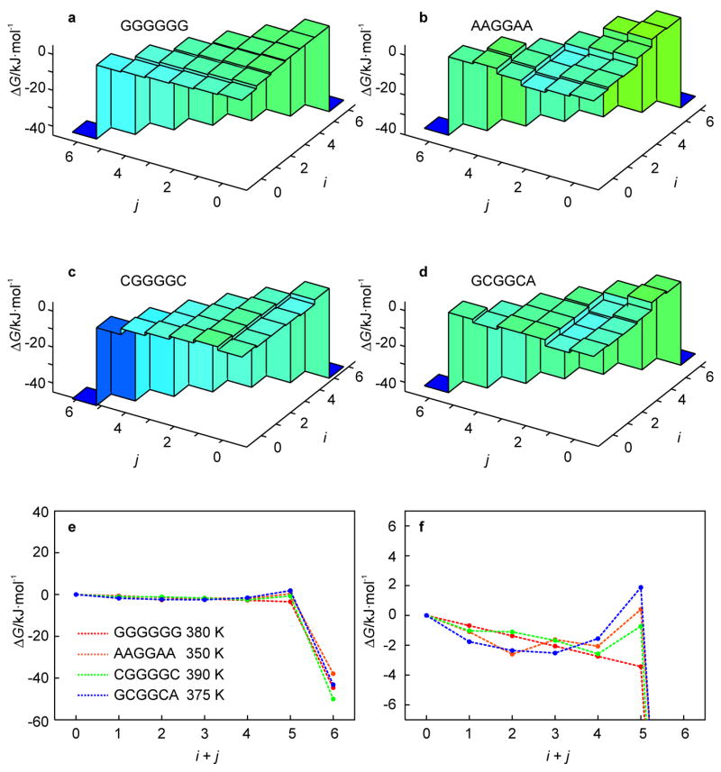
Effect of stem sequence permutations, Fig. 1d–g, of the hairpin of Fig. 1c (n = 13) on the free energy landscape as obtained from the KIS model (a–d). (Un)folding pathways characteristic of the above landscapes are represented by 1D profiles (e). The behavior for i + j < 6 is magnified in the lower right panel to illustrate the change in the unfolding barrier (f).

For a heterogeneous stem sequence, pairing and stacking inequalities can create valleys and local minima on the energy landscape, which can be further decreased or increased by ΔG_loop(i, j). Significantly, this stem-sequence survey shows that the temperature-dependent non-two-state kinetics is a general phenomenon. For most sequences, inhomogeneities in the stacking enthalpies in the stem are significantly smaller than ΔG_loop(i, j), the increase in free energy due to unzipping from the loop end. In such cases, the kinetic behavior follows a simple rule: the most favorable unfolding trajectory is simply to unzip from the loop end if the free end is terminated by a G-C base pair and the loop end is terminated by an A-T base pair. Otherwise, unzipping from the free end is more favorable. This is exemplified by the stem sequence permutation shown in Fig. 1e, and its corresponding landscape in Fig. 6b.

base pairing inequalities become important and affect the free energy landscape for some stem sequences. For example, Fig. 1f shows a stem sequence for which ΔG_loop(i, j) is smaller than the differences in stacking free energy. The stem consists only of G-C base pairs. However, 5′-GC-3′ stacking is more favorable than 5′-CG-3′ or 5′-GG-3′ stacking. This difference in stacking enthalpy is larger than ΔG_loop(i, j). Therefore, instead of unzipping from the free end, the hairpin unzips from the loop end until it reaches the state (4, 0) (Fig. 6c). At this point, unzipping from the loop or free end of the stem involves disrupting 5′-GC-3′ stacking so that unzipping from the free end is favored. As another example, Fig. 1g shows a sequence for which the CG stacking interactions at the free end are especially weak whereas the AC stacking interactions at the loop end are especially strong. In addition, since the loop entropy ΔG_loop(i, j) favors smaller loops, this leads to disruption of the G-C base pair at the free end before the A-T base pair at the loop end (Fig. 6d). However, regardless of the specific sequence effects, the general temperature-dependent kinetic behavior predicted by the model supports the findings of a recent time-resolved UV spectroscopic study on the RNA hairpin GC-UUUU-GC, in which the “two-state” destacking kinetics observed at T = T_m is replaced by three-state kinetics at higher temperatures T > T_m.[12]

The effect of the loop size on the free energy landscape is depicted in Fig. 7. The stem sequence was kept fixed to that of the benchmark hairpin and the loop size was varied between 5 and 40 nucleotides (Fig. 1c). The free-energy landscapes of all loop variants are shown for T = 360 K, which is the temperature at which the kinetic intermediate state of the benchmark hairpin is most pronounced. The profiles of the most likely unfolding pathway, Fig. 7e, demonstrate that the free energy of the unfolded state (i + j = 6) decreases with increasing loop size. However, this effect becomes less pronounced for longer loops. This is because the negative conformational entropy due to loop closure increases in magnitude with increasing loop size, while the rate of change in the magnitude decreases with increasing loop size. Consequently, the gradient from (0, 0) to the intermediate state (2, 0) becomes steeper for longer loops (Fig. 7f). For n = 20 and 40, the entropic penalty due to an increase in loop length is small and the valley in the free energy landscape originates from the unzipping of the weaker A-T base pairs at the loop end. For n = 5 and 10, the entropic penalty of loop expansion is larger and offsets the relative weakness of A-T base pairing, leading to more shallow valleys. Thus, the loop length affects the free energy difference between the native hairpin and the unfolded ensemble (which determines T_m) as well as the depth of the intermediate valley on the free energy landscape. However, for n > 10, the loop length only scales these features but does not create new topological features on the free energy landscape.

Fig. 7.

Effect of the loop length on the free energy landscape of the hairpin of Fig. 1c (5 ≤ n ≤ 40) as obtained from the KIS model (a–d). (Un)folding pathways characteristic of the above landscapes are represented by 1D profiles (e). The behavior for i + j < 6 is magnified in the lower right panel to illustrate the change in the unfolding barrier (f).

Conclusion

Stimulated by recent ultrafast T-jump experiments from this laboratory, here we introduced the kinetic intermediate structure (KIS) model, a two-coordinate free energy landscape model describing the energetics and kinetics of hairpin melting. The model was tested against molecular dynamics simulations, and the results of both methods were evaluated in the light of recent experimental findings. Significantly, the model, although simple, predicts the existence, as well as the specific base pairing configuration, of intermediate states along the path of unfolding. Thus, the model provides the relevant, structurally-specific, kinetic behavior for the macromolecule. For a range of final temperatures above the melting temperature, intermediate states of collapsed structures emerge as local valleys with lower free energy than the native hairpin state, but separated from the unfolded-state global minimum by a significant barrier, leading to non-two-state dynamics (Figs. 2, 4, and 5). The approximations and predictions of the model are confirmed by MD simulations as illustrated in Figs. 3, 4, and 8. In addition, the model supports the existence of stem-sequence and temperature-dependent intermediates also observed for RNA hairpins.

Fig. 8.

Spatiotemporal snapshots of an unfolding trajectory of the hairpin of Fig. 1a as obtained from MD simulations. The time elapsed and the (i, j)-assignment are presented for each snapshot. Notably, the stem end of the hairpin undergoes a repeated reversible (un)zipping during the course of unfolding, which is common among the MD trajectories for all temperatures reported here.

In general, for hairpin unfolding, we conclude that (i) the unfolding kinetics can be non-two-state for a range of T-jumps, (ii) the stem sequence determines the identity of the kinetic intermediate and the most likely unfolding pathway, and (iii) the hairpin loop length affects the depth of the local minima on the free energy landscape. The interplay of enthalpic and entropic contributions to the free energy plays a significant role in creating intermediates, not only in biological systems, but also for mesoscopic structures such as clusters of atoms; for example, the creation of valleys of local stability has been addressed for the liquid-like to solid-like transitions in argon clusters.[51]

The KIS model can be extended in both detail and scope. In the current case, all unfolded structures are grouped into a single unfolded state, which corresponds to the diagonal points on the free energy landscape (Fig. 1b). However, the model can be extended, for example, by setting the diagonal points (i, 6 –i) to correspond to the unfolded state for which the nucleotides that form the i-th contact from the loop end are within some threshold distance of each other. In this way, the free energy landscape can also accommodate collapsed but totally unfolded structures as well. Moreover, the KIS model may be employed to understand the sequence-dependent kinetics of other biomolecular structures that may satisfy the SSA and RSA, such as polypeptide α-helices and β-strands, but now with the structural configurations well defined. The essential mechanisms distilled by the model are illustrative of the key insights possible with well-chosen coarse-graining models of macromolecular (protein) folding.[52]

References

- 1.Brion P, Westhof E. Annu Rev Biophys Biomol Struct. 1997;26:113–137. doi: 10.1146/annurev.biophys.26.1.113. [DOI] [PubMed] [Google Scholar]
- 2.Varani G. Annu Rev Biophys Biomol Struct. 1995;24:379–404. doi: 10.1146/annurev.bb.24.060195.002115. [DOI] [PubMed] [Google Scholar]
- 3.Glucksmann-Kuis MA, Dai X, Markiewicz P, Rothman-Denes LB. Cell. 1996;84:147–154. doi: 10.1016/s0092-8674(00)81001-6. [DOI] [PubMed] [Google Scholar]
- 4.Lodish H, Berk A, Zipursky SL, Matsudaira P, Baltimore D, Darnell JE. Molecular Cell Biology. 4. W. H. Freeman; New York: 2000. [Google Scholar]
- 5.Uhlenbeck OC. Nature. 1990;346:613–614. doi: 10.1038/346613a0. [DOI] [PubMed] [Google Scholar]
- 6.Zhang W, Chen SJ. Proc Natl Acad Sci USA. 2002;99:1931–1936. doi: 10.1073/pnas.032443099. [DOI] [PMC free article] [PubMed] [Google Scholar]
- 7.Sorin EJ, Rhee YM, Nakatani BJ, Pande VS. Biophys J. 2003;85:790–803. doi: 10.1016/S0006-3495(03)74520-2. [DOI] [PMC free article] [PubMed] [Google Scholar]
- 8.Kannan S, Zacharias M. Biophys J. 2007;93:3218–3228. doi: 10.1529/biophysj.107.108019. [DOI] [PMC free article] [PubMed] [Google Scholar]
- 9.Bonnet G, Krichevsky O, Libchaber A. Proc Natl Acad Sci USA. 1998;95:8602–8606. doi: 10.1073/pnas.95.15.8602. [DOI] [PMC free article] [PubMed] [Google Scholar]
- 10.Jung J, Van Orden A. J Am Chem Soc. 2006;128:1240–1249. doi: 10.1021/ja0560736. [DOI] [PubMed] [Google Scholar]
- 11.Goddard NL, Bonnet G, Krichevsky O, Libchaber A. Phys Rev Lett. 2000;85:2400–2403. doi: 10.1103/PhysRevLett.85.2400. [DOI] [PubMed] [Google Scholar]
- 12.Ma H, Proctor DJ, Kierzek E, Kierzek R, Bevilacqua PC, Gruebele M. J Am Chem Soc. 2006;128:1523–1530. doi: 10.1021/ja0553856. [DOI] [PubMed] [Google Scholar]
- 13.Ansari A, Kuznetsov SV, Shen Y. Proc Natl Acad Sci USA. 2001;98:7771–7776. doi: 10.1073/pnas.131477798. [DOI] [PMC free article] [PubMed] [Google Scholar]
- 14.Ma H, Wan C, Wu A, Zewail AH. Proc Natl Acad Sci USA. 2007;104:712–716. doi: 10.1073/pnas.0610028104. [DOI] [PMC free article] [PubMed] [Google Scholar]
- 15.Enderlein J. ChemPhysChem. 2007;8:1607–1609. doi: 10.1002/cphc.200700247. [DOI] [PubMed] [Google Scholar]
- 16.Miller TF, III, Vanden-Eijnden E, Chandler D. Proc Natl Acad Sci USA. 2007;104:14559–14564. doi: 10.1073/pnas.0705830104. [DOI] [PMC free article] [PubMed] [Google Scholar]
- 17.Zhang W, Chen SJ. J Chem Phys. 2001;114:7669–7681. [Google Scholar]
- 18.Thompson PA, Eaton WA, Hofrichter J. Biochemistry. 1997;36:9200–9210. doi: 10.1021/bi9704764. [DOI] [PubMed] [Google Scholar]
- 19.Ivanov V, Zeng Y, Zocchi G. Phys Rev E. 2004;70:051907. doi: 10.1103/PhysRevE.70.051907. [DOI] [PubMed] [Google Scholar]
- 20.Ares S, Voulgarakis NK, Rasmussen KØ, Bishop AR. Phys Rev Lett. 2005;94:035504. doi: 10.1103/PhysRevLett.94.035504. [DOI] [PubMed] [Google Scholar]
- 21.Kuznetsov SV, Shen Y, Benight AS, Ansari A. Biophys J. 2001;81:2864–2875. doi: 10.1016/S0006-3495(01)75927-9. [DOI] [PMC free article] [PubMed] [Google Scholar]
- 22.Poland D, Scheraga HA. Theory of Helix-Coil Transitions in Biopolymers: Statistical Mechanical Theory of Order-Disorder Transitions in Biological Macromolecules. 1. Academic Press; New York: 1970. [Google Scholar]
- 23.Wartell RM, Benight AS. Phys Rep. 1985;126:67–107. [Google Scholar]
- 24.Paner TM, Amaratunga M, Doktycz MJ, Benight AS. Biopolymers. 1990;29:1715–1734. doi: 10.1002/bip.360291405. [DOI] [PubMed] [Google Scholar]
- 25.Klump H, Ackermann T. Biopolymers. 1971;10:513–522. doi: 10.1002/bip.360100307. [DOI] [PubMed] [Google Scholar]
- 26.Frank-Kamenetskii MD. Biopolymers. 1971;10:2623–2624. doi: 10.1002/bip.360101223. [DOI] [PubMed] [Google Scholar]
- 27.SantaLucia J., Jr Proc Natl Acad Sci USA. 1998;95:1460–1465. doi: 10.1073/pnas.95.4.1460. [DOI] [PMC free article] [PubMed] [Google Scholar]
- 28.Petersheim M, Turner DH. Biochemistry. 1983;22:256–263. doi: 10.1021/bi00271a004. [DOI] [PubMed] [Google Scholar]
- 29.Yamakawa H, Stockmayer WH. J Chem Phys. 1972;57:2843–2854. [Google Scholar]
- 30.Mills JB, Vacano E, Hagerman PJ. J Mol Biol. 1999;285:245–257. doi: 10.1006/jmbi.1998.2287. [DOI] [PubMed] [Google Scholar]
- 31.SantaLucia J, Jr, Hicks D. Annu Rev Biophys Biomol Struct. 2004;33:415–440. doi: 10.1146/annurev.biophys.32.110601.141800. See also: supplementary materials therein. [DOI] [PubMed] [Google Scholar]
- 32.Hilbers CW, Haasnoot CA, de Bruin SH, Joordens JJ, van der Marel GA, van Boom JH. Biochimie. 1985;67:685–695. doi: 10.1016/s0300-9084(85)80156-5. [DOI] [PubMed] [Google Scholar]
- 33.Haasnoot CA, Hilbers CW, van der Marel GA, van Boom JH, Singh UC, Pattabiraman N, Kollman PA. J Biomol Struct Dyn. 1986;3:843–857. doi: 10.1080/07391102.1986.10508468. [DOI] [PubMed] [Google Scholar]
- 34.Paner TM, Amaratunga M, Benight AS. Biopolymers. 1992;32:881–892. doi: 10.1002/bip.360320714. [DOI] [PubMed] [Google Scholar]
- 35.van Dongen MJP, Mooren MMW, Willems EFA, van der Marel GA, van Boom JH, Wijmenga SS, Hilbers CW. Nucl Acids Res. 1997;25:1537–1547. doi: 10.1093/nar/25.8.1537. [DOI] [PMC free article] [PubMed] [Google Scholar]
- 36.Berman HM, Westbrook J, Feng Z, Gilliland G, Bhat TN, Weissig H, Shindyalov IN, Bourne PE. Nucl Acids Res. 2000;28:235–242. doi: 10.1093/nar/28.1.235. [DOI] [PMC free article] [PubMed] [Google Scholar]
- 37.Jorgensen WL, Chandrasekhar J, Madura JD, Impey RW, Klein ML. J Chem Phys. 1983;79:926–935. [Google Scholar]
- 38.Berendsen HJC, van der Spoel D, van Drunen R. Comput Phys Commun. 1995;91:43–56. [Google Scholar]
- 39.Lindahl E, Hess B, van der Spoel D. J Mol Model. 2001;7:306–317. [Google Scholar]
- 40.Kaminski GA, Friesner RA, Tirado-Rives J, Jorgensen WL. J Phys Chem B. 2001;105:6474–6487. [Google Scholar]
- 41.Sorin EJ, Pande VS. Biophys J. 2005;88:2472–2493. doi: 10.1529/biophysj.104.051938. [DOI] [PMC free article] [PubMed] [Google Scholar]
- 42.Essmann U, Perera L, Berkowitz ML, Darden T, Lee H, Pedersen LG. J Chem Phys. 1995;103:8577–8593. [Google Scholar]
- 43.Nosé S. Mol Phys. 1984;52:255–268. [Google Scholar]
- 44.Hoover WG. Phys Rev A. 1985;31:1695–1697. doi: 10.1103/physreva.31.1695. [DOI] [PubMed] [Google Scholar]
- 45.Parrinello M, Rahman A. J Appl Phys. 1981;52:7182–7190. [Google Scholar]
- 46.Nosé S, Klein ML. Mol Phys. 1983;50:1055–1076. [Google Scholar]
- 47.Berendsen HJC, Postma JPM, van Gunsteren WF, DiNola A, Haak JR. J Chem Phys. 1984;81:3684–3690. [Google Scholar]
- 48.Hess B, Bekker H, Berendsen HJC, Fraaije JGEM. J Comput Chem. 1997;18:1463–1472. [Google Scholar]
- 49.Miyamoto S, Kollman PA. J Comput Chem. 1992;13:952–962. [Google Scholar]
- 50.The experimental solvent consisted of 50 mM sodium and 30 mM phosphate, while the parameters used in the KIS-model are for 100 mM NaCl.
- 51.Berry RS. In: Strength from Weakness: Structural Consequences of Weak Interactions in Molecules, Supermolecules, and Crystals, ch 8. Domenicano A, Hargittai I, editors. Kluwer Academic Publishers; Amsterdam: 2002. pp. 143–168. [Google Scholar]
- 52.Clementi C. Curr Opin Struct Biol. 2008;18:10–15. doi: 10.1016/j.sbi.2007.10.005. [DOI] [PubMed] [Google Scholar]