

Abstract
The implementation of molecular dynamics (MD) with our physics-based protein united-residue (UNRES) force field, described in the accompanying paper (Khalili et al. J. Phys. Chem. B 2005, 109, 13785), was extended to Langevin dynamics. The equations of motion are integrated by using a simplified stochastic velocity Verlet algorithm. To compare the results to those with all-atom simulations with implicit solvent in which no explicit stochastic and friction forces are present, we alternatively introduced the Berendsen thermostat. Test simulations on the Ala10 polypeptide demonstrated that the average kinetic energy is stable with about a 5 fs time step. To determine the correspondence between the UNRES time step and the time step of all-atom molecular dynamics, all-atom simulations with the AMBER 99 force field and explicit solvent and also with implicit solvent taken into account within the framework of the generalized Born/surface area (GBSA) model were carried out on the unblocked Ala10 polypeptide. We found that the UNRES time scale is 4 times longer than that of all-atom MD simulations because the degrees of freedom corresponding to the fastest motions in UNRES are averaged out. When the reduction of the computational cost for evaluation of the UNRES energy function is also taken into account, UNRES (with hydration included implicitly in the side chain–side chain interaction potential) offers about at least a 4000-fold speed up of computations relative to all-atom simulations with explicit solvent and at least a 65-fold speed up relative to all-atom simulations with implicit solvent. To carry out an initial full-blown test of the UNRES/MD approach, we ran Berendsen-bath and Langevin dynamics simulations of the 46-residue B-domain of staphylococcal protein A. We were able to determine the folding temperature at which all trajectories converged to nativelike structures with both approaches. For comparison, we carried out ab initio folding simulations of this protein at the AMBER 99/GBSA level. The average CPU time for folding protein A by UNRES molecular dynamics was 30 min with a single Alpha processor, compared to about 152 h for all-atom simulations with implicit solvent. It can be concluded that the UNRES/MD approach will enable us to carry out microsecond and, possibly, millisecond simulations of protein folding and, consequently, of the folding process of proteins in real time.
1. Introduction
In the accompanying paper,1 we derived the Lagrange equations of motion for the united-residue (UNRES) force field for protein simulations.2–16 We applied the velocity Verlet algorithm to integrate the equations of motion and tested the symplectic properties of the algorithm by running microcanonical simulations on the Ala10 polypeptide. The algorithm appears to be stable up to about a 1 fs time step; however, some energy drift appears because of instability of the gradient of the present side-chain-rotamer (Urot) contribution to UNRES; this component must ultimately be replaced with one leading to stable gradients. To reduce the energy drift and, thereby, to increase the time step further, we developed a variable-time-step algorithm in which the time step is scaled down if the change in acceleration exceeds a cutoff value. With this modification, the algorithm is stable up to about a 2.5 fs time step.
In this paper, we introduce Langevin dynamics with the UNRES force field to take into account the dynamic effects of the solvent and also to couple the system under study to a thermal bath. To compare the results of the simulations with those of all-atom studies reported here and in the literature,17 which were carried out at the all-atom level with implicit solvent, we also introduce the Berendsen thermostat, where the friction and random forces are present only implicitly. We carry out test simulations on the Ala10 polypeptide and the B-domain of staphylococcal protein A, a 46-residue protein with a three-helix-bundle topology, and compare the results with those of all-atom simulations to determine the relation between the UNRES and the all-atom time scale.
2. Methods
2.1. Langevin Dynamics with the UNRES Force Field
The UNRES force field is outlined in the accompanying paper1 and also described in detail in our earlier work.2–16 Briefly, a polypeptide chain is represented as a sequence of α-carbon atoms (Cα's). The Cα's are linked together by virtual bonds (designated as dCs), which constitute the backbone. The interaction sites are the united peptide groups (p's) in the middle of the dCs, and the united side chains at the ends of virtual bonds are designated as dXs. The p centers represent only the C′, O, N, and H atoms of the peptide groups, while the Cα atoms are included in the SC centers. Consequently, the positions of the Cα atoms are only geometric points. The energy of a united-residue chain is derived as a restricted free energy (RFE) function (or potential of mean force (PMF)) obtained by computing the free energy corresponding to a given coarse-grain conformation by integrating out those degrees of freedom that are not considered in the UNRES model.7,13 The force field has been optimized by our novel hierarchical-optimization method11,14–16 in which the energy of a training protein is required to decrease with native likeness increasing in an ordered way that corresponds to the experimentally observed folding pathway, if such information is available from experiment. In this work, we use the force field derived using 1IGD (a 61-residue α + β-protein);15 this force field is referred to as the F2 force field.
In the accompanying paper,1 we derived the Lagrange equations of motion for the UNRES model. We chose the components of the Cα⋯Cα and Cα⋯SC virtual-bond vectors as the generalized coordinates, the vector of generalized coordinates being defined as q = (dCo, dCs, …, dCe−1, dXi1, …, dXim)T, where dCi denotes the vector pointing from to and dX denotes the vector pointing from to SCi with dCo defining the absolute position of the first Cα atom, i1, i2, …, im denote the numbers (m) of non-glycine residues, while s and e are the number of the first and the last nondummy Cα atom, respectively. The entries corresponding to glycine residues are omitted from the list of dXs because, for a glycine residue, the position of its “side chain” coincides with that of the respective Cα atom.2 The “dummy” Cα atoms are introduced if the first (last) residue is not glycine and if the chain is unblocked;2 this is necessary to define the local reference frame for the first (last) side chain. If the first residue is a dummy, then s = 2; otherwise s = 1. If the last residue is a dummy, then e = n − 1; otherwise e = n. We assumed that the virtual bonds are flexible rods with uniformly distributed masses. The number of dX vectors is equal to the number of residues minus the number of glycine residues in a chain. The Cartesian coordinates of the interacting sites x = (xps, xps+1, …xpe−1, xSCs, xSCs+1, …, xSCe)T and their velocities v = (vps, vps+1, …vpe−1, vSCs, vSCs+1, …, vSCe)T are related to the generalized coordinates q and generalized velocities q̇ by eqs 1 and 2, respectively.1 It should be noted that all side chains (including the “side chains” of glycine residues that are centered at the Cα atoms) are included in the vectors x and v.
| (1) |
| (2) |
with A being the transformation matrix from the generalized coordinates (q) to the Cartesian coordinates (x) of the sites. The matrix A is defined by eq 27 of the accompanying paper.1
On the basis of eq 9 and eqs 19–25 of the accompanying paper,1 we can write the Langevin equations for the UNRES model as eq 3.
| (3) |
with the inertia matrix G defined by eq 4.
| (4) |
where U is the UNRES potential energy, ffric and frand are the friction and random forces, respectively, M (defined by eq 28 of the accompanying paper1) is the diagonal matrix of the masses of the interacting sites, and H (defined by eq 29 of the accompanying paper1) is the part of the inertia matrix that corresponds to the internal (stretching) motions of the virtual bonds.
We use Stokes law18 to compute the friction forces. In this work, we assume that each interacting site behaves as a sphere moving through water. Of course, a more refined treatment should take into account at least the ellipsoidal shape of a site, but we leave this to further work. Further, we assume that the friction force is proportional to the solvent-accessible surface area of a site, following the suggestion of other authors.19 Thus, the friction force acting on site z is expressed by eq 5.
| (5) |
with
| (6) |
where γz is the friction coefficient of site z, vz is the velocity vector of site z, rz is the effective radius of site z, rwat is the effective radius of water (taken in this study as 1.4 Å), ηwat is the viscosity of water equal to 0.8904 cpoise at 298 K, Sz is the solvent-accessible surface area of site z, and α is a scaling factor. We used the radii computed by Levitt20 for the radii of the side chains, while the effective radius of the peptide group was set at 5 Å, based on the van der Waals radius of the peptide group estimated from high-level ab initio quantum-mechanical calculations of the energy surfaces of interacting peptide groups.13 We adapted the algorithm21,22 from the TINKER package23,24 to calculate the surface area. Because the surface area of the UNRES sites often happens to decrease to zero, we set a lower limit of 0.1 on the ratio of the solvent-accessible surface area of a site to its total surface area (eq 6). The scaling factor α is introduced to reduce the friction and random forces, which would otherwise be more than an order of magnitude higher than the forces of the potential. From the work of other authors (see, e.g., the Appendix in ref 25), α should range from 0.001 (low-friction limit) to 0.1 (overdamped limit).
On the basis of eq 1, we can convert the forces expressed in the Cartesian coordinates of the interacting sites, fx, into forces expressed in the generalized coordinates, fq, by using eq 7.
| (7) |
Through the use of eqs 2 and 7, we can convert the friction forces expressed in the Cartesian coordinates of the sites (eq 5) into the friction forces expressed in generalized coordinates
| (8) |
The friction matrix Γ is a diagonal matrix (eq 9) whose elements are calculated from Stokes law18 modified by the dependence of the friction coefficients on the solvent-accessible surface area19 according to eq 6.
| (9) |
where 1 is a 3 × 3 identity matrix and 0 is a 3 × 3 matrix composed of zeros. Thus, even though the friction acting on individual sites is assumed to be isotropic, the friction matrix (ATΓA) in the generalized coordinates q is not diagonal.
The random forces acting on interaction sites are δ-correlated forces, i.e., cov[frand(t1), frand(t2)] ∝ δ(t2 − t1) at times t1 and t2 of the trajectory (where cov denotes the covariance and δ the Kronecker δ function), which are expressed at every integration step by eq 10.25–27
| (10) |
where is the vector of random forces acting on site z, γz is the friction coefficient of this site (defined by eq 6), R is the universal gas constant, T is the absolute temperature, δt is the integration time step, and N(0,1) is the three-dimensional vector whose components are sampled independently from a normal distribution with zero mean and unit variance. Together, the stochastic and friction forces constitute a thermostat that maintains the average temperature at the preset value.
Again, by using eq 7, we can transform the random forces from the Cartesian coordinates of the interacting sites to the generalized coordinates, which yields eq 11.
| (11) |
2.2. Integrating the Langevin Equations of Motion by the Velocity Verlet Algorithm
A variety of stochastic integrators have been developed for Langevin dynamics, most of them being stochastic versions of of the leapfrog28–31 and the velocity Verlet32–34 algorithm. These algorithms are based on stochastic differential equation theory and perform analytical integration of the friction and the stochastic forces in a single time step. An elegant way of deriving the algorithms for Langevin dynamics makes use of the Liouville propagator and the Suzuki formula35 for time-ordered exponentials; this is the basis of the algorithms developed by Ciccotti and co-workers.36,37 Their formulas are slightly different from those developed earlier.
In the Appendix, we describe in detail our adaptation of the procedure from the TINKER package23,24 described in refs 32 and 33. However, we note that the stochastic integrator from TINKER as well as all stochastic integrators described in the papers cited above involve a tremendous increase of computational cost compared to microcanonical calculations with UNRES. The reason for this is that the exponentials of the friction matrix must be calculated, as opposed to the case of diagonal equations of motion when exponentials of the friction coefficients (scalars) are calculated. For not too large friction coefficients and not too large time steps, which is the case of our work, the matrix exponentials can be expanded into a power series, and only the first-order terms can be considered without loss of accuracy. If this is done and if all terms with δt2 and higher are ignored in the expressions for new velocities and all terms with δt3 and higher in the expressions for new coordinates, then the algorithm from TINKER32,33 and the algorithm of Ciccotti et al.36,37 reduce to the velocity Verlet algorithm with stochastic and friction forces included. This algorithm can be summarized as follows:
Step 1 (updating coordinates):
| (12) |
Step 2 (updating velocities):
| (13) |
with
| (14) |
| (15) |
| (16) |
| (17) |
and the subscripts “x” and “v” at q̈rand indicating that the random forces are sampled independently to compute the new coordinates and velocities, respectively.
The simplified stochastic velocity Verlet algorithm (eqs 2 and 13) does not involve the computation of matrix exponentials and is, therefore, much more practical than the original integrators for the case of nondiagonal equations of motion implied in UNRES dynamics. We found that the simplified algorithm does not differ in performance (i.e., maintaining the average temperature, the value of the variance of the potential and the kinetic energy, and the velocity autocorrelation function) from the original algorithm from TINKER32,33 and the algorithm introduced by Ciccotti.36,37
2.3. Berendsen's Thermostat
To carry out canonical simulations in the simplest possible manner, we implemented Berendsen's method to couple the system to a thermal bath.38 This method is based on the Langevin equations, which are solved approximately at a given time step. Instead of using the simplified stochastic velocity Verlet algorithm (eqs 12–17), the velocities computed in the second step of the regular velocity Verlet algorithm (eq 31 of ref 1) are scaled by the factor λ defined by eq 18.
| (18) |
where δt is the time step, To is the desired temperature, and T(t) is the instantaneous temperature of the system at time t, which is calculated from eq 19.
| (19) |
where K(t) is the total kinetic energy of the system at time t, R is the universal gas constant, and Nf is the number of degrees of freedom in the system, which is equal to 3np + 3nSC − 3nGly where np is the number of peptide groups, nSC is the number of side chains, and nGly is the number of glycine residues in the system. The parameter τT is a measure of the strength of the coupling to the thermal bath. For values of τT much larger than δt, the simulation is reduced to a microcanonical ensemble. It was shown38 that, for small values of τT relative to δt, the fluctuations in the kinetic energy are reduced at the expense of an increase in the fluctuations of the potential and total energy. Although small values of τT influence fluctuations, average thermodynamic quantities are not disturbed even for very small τT values.38 However, the fluctuations of global properties are strongly influenced for small coupling time constants, and their intensity cannot be used to derive thermodynamic properties.
At the end of every full velocity Verlet step, the velocities are scaled, following eq 20.
| (20) |
The advantage of the Berendsen algorithm is that the coupling strength can be made as weak as possible to reduce the disturbance of the system. This algorithm is numerically stable, and truncation errors will not develop undesired deviations that would require further correction. This is especially important for long runs and is also fairly easy to implement. A disadvantage of the Berendsen algorithm is that it does not always give correct values of thermodynamic quantities.
An undesirable feature of the Berendsen-type runs is that, as the molecule relaxes (i.e., loses its potential energy), the kinetic energy is converted into net rotation of the whole molecule. To overcome this problem, we reset the angular momentum of the molecule to zero every 1000 time steps.
2.4. All-Atom Molecular Dynamics Simulations of the Ala10 and Protein A System
For ultimate comparison of the time step in all-atom and UNRES calculations, we carried out all-atom molecular dynamics (MD) simulations of the unblocked Ala10 polypeptide with the AMBER 99 force field.39,40 A series of nine simulations was carried out in a periodic box of water with 3155 water molecules in the NPT ensemble (constant number of particles, pressure, and temperature) at T = 298 K and P = 1 atm. An 8-Å cutoff was applied to nonbonded interactions, and the particle-mesh Ewald summation was applied to evaluate electrostatic interactions. The TIP3P41 model of water was used. The SHAKE42,43 algorithm was used to maintain the valence geometry of the water molecules.
To compare the time scale of UNRES/MD with that of implicit solvent all-atom MD, we ran a series of 10 MD all-atom simulations on the unblocked Ala10 polypeptide with the AMBER 99 force field with the solvent treated with the generalized Born model.44,45 The system was coupled to a thermal bath by using the Berendsen algorithm38 with the coupling parameter τT = 0.1 ps. The simulations were carried out at a temperature T = 400 K, and the integration time step was δt = 2 fs. A distance cutoff of 20 Å was applied to evaluate all nonbonded interactions in both series of all-atom simulations.
As a second set of calculations to characterize the time step with the UNRES model, we carried out all-atom MD simulations of the 46-residue N-terminal fragment of the B-domain of staphylococcal protein A46 with the sequence Ac-Gln-Gln-Asn-Ala-Phe-Tyr-Glu-Ile-Leu-His-Leu-Pro-Asn-Leu-Asn-Glu-Glu-Gln-Arg-Asn-Gly-Phe-Ile-Gln-Ser-Leu-Lys-Asp-Asp-Pro-Ser-Gln-Ser-Ala-Asn-Leu-Leu-Ala-Glu-Ala-Lys-Lys-Leu-Asn-Asp-Ala-NHMe; the AMBER 99/GBSA force field at temperatures T = 300, 320, 350, 400, 420, 450, and 500 K, with a coupling parameter τT = 1 ps, was used. The other settings were the same as for all-atom simulations of Ala10 with implicit solvent. Five trajectories, starting from a fully extended chain, were run for each temperature, and the duration of a run was 20 ns.
3. Results and Discussion
3.1. Equilibrium and Folding Simulations of the Ala10 Polypeptide
To carry out initial tests of the UNRES/MD approach to protein folding, we ran simulations on the Ala10 polypeptide, using the Berendsen thermostat and full-blown Langevin equations, respectively. To run simulations with the Berendsen thermostat, we had to choose the value of the coupling parameter τT. In all-atom simulations, the coupling parameter τT of eq 18 usually ranges from 0.5 to 5 ps, and even values from 0.1 ps and higher result in stable trajectories38 and reliable values of thermodynamic properties. However, this information cannot be implemented directly in the UNRES/MD approach because the time scale of a united-residue chain need not be the same as for an all-atom chain. We, therefore, ran a series of test simulations on the Ala10 polypeptide to determine the plausible value of τT. The global minimum of the UNRES potential energy with the F2 force field of ref 15 is a full right-handed α-helix with potential energy equal to −44.8 kcal/mol. We wanted to satisfy three criteria: (i) the fluctuations of the kinetic, potential, and total energy should be reasonably small, (ii) the folding time should be short, and (iii) the native structure should be reasonably stable. Criteria i and iii somehow overlap because, with increasing energy fluctuations, the system must leave the native structure frequently and visit different regions of conformational space. Criterion ii ensures that the coupling is strong enough because, for large values of τT, we approach the microcanonical mode in which Ala10 does not fold fully because of accumulation of too much kinetic energy as the potential energy decreases.
The first simulations were started from the α-helical conformation of Ala10 (with θ = 90°, γ = 45°, α = 120°, and β = −120° for all residues). We ran simulations at T = 300 K with the time steps 0.01 mtu (0.489 fs), 0.02 mtu (0.978 fs), 0.04 mtu (1.956 fs), and 0.1 mtu (4.89 fs). The duration of a simulation was 4000 mtu (196 ps). Ten trajectories were run for each value of τT and each time step. The standard deviations of the potential, kinetic, and total energy were computed after discarding the initial 10 ps equilibration period. The standard deviations (σ) of the energies as well as the actual temperature averaged over all trajectories for a given time step and a given τT are plotted versus τT in Figure 1. Figure 1 shows that, for small values of τT, the fluctuations in the kinetic energy are small, while those in the potential and total energy are large. For larger values of τT, the fluctuations in the kinetic energy increase while those of the potential energy reach minima at τT between 5 and 10 mtu (Figure 1A). The depth of these minima increases with the time step, which strongly suggests that they are caused by energy drift due to integration errors; this energy drift is remarkable when the coupling is weak, and consequently, the system approaches the behavior of a microcanonical system. Therefore, τT larger than 10 mtu should not be used with larger time steps. It can also be noted that, for the largest time step (0.1 mtu), the average temperature deviates significantly from the set value for τT > 5 mtu (Figure 1B); therefore, with this large time step, one should be careful to introduce tight coupling (i.e., set a small value of τ). The fluctuations of the kinetic, potential, and the total energy become comparable for τT = 5 mtu (0.2445 ps); for all-atom simulations, this is a good criterion for selection of τT, because one can obtain reliable values of observables and their fluctuations.38 However, we must bear in mind that there is no explicit solvent in UNRES, and therefore, in reality, the potential and the total energy can fluctuate more because the molecule exchanges energy with the surrounding solvent, which has to be simulated by the Berendsen thermostat.
Figure 1.
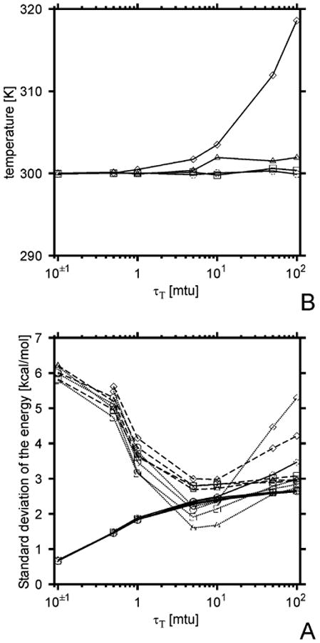
Plots of the standard deviation in the kinetic (σT, solid lines), the potential (σV, dashed lines), and the total (σE, dotted lines) energy (A), and average temperature (kinetic energy, B), as functions of the coupling parameter τT for different values of the time step δt. Simulations were carried out on the Ala10 system, starting from the fully α-helical structure and 10 200-ps trajectories were run for each δt and each τT value. The symbols correspond to the values of the time step: circles, δt = 0.01 mtu (0.489 fs); squares, δt = 0.02 mtu (0.978 fs); triangles, δt = 0.05 mtu (2.445 fs); diamonds, δt = 0.10 mtu (4.89 fs).
The next series of simulations to estimate a plausible value of τT were the folding simulations of the Ala10 polypeptide, starting from the fully extended chain (θ = 110°, γ = 180°, α = 110°, and β = −120° for all residues). We ran 1 000 000-step (1956 ns) simulations at T = 300 K with δt = 0.04 mtu (1.956 fs) and for τT = 0.1, 0.5, 1.0, 2.0, and 5.0 mtu. Ten trajectories were run for each τT value. To monitor the progress of folding, we computed the Cα root-mean-square deviation (rmsd) from that of the Ala10 all-atom chain in an ideal α-helix conformation minimized with the ECEPP/3 all-atom force field.47 Because the ends of the chain are subject to much greater fluctuations than those of the inner residues, only residues from 2 to 9 were superposed in computing the rmsd; we found that this provided a much clearer analysis of the folding trajectory compared to the rmsd over all residues. The analyzed rmsd will hereafter be referred to as ρα.
To characterize the folding of Ala10, we followed our earlier work on force-field optimization14 and, for trajectory i, defined the folding time, , as the time when ρα first decreased below 1 Å and the stability time, , as the total length of those parts of a trajectory after τf where ρα was not larger than 2 Å. For trajectories in which the peptide did not fold (i.e., ρα did not decrease below 1 Å), τf was considered to take on the length of a trajectory. We also defined the stability (τs/t) as the ratio of τs to the length of the trajectory (t).
The average folding (τf) and stability (τs) times (over 10 trajectories) are plotted against the coupling constant τT in Figure 2, while sample plots of the potential energy, temperature, and ρα for five representative trajectories corresponding to τT = 1 mtu are shown in Figure 3. It can be seen that the potential energy is always higher by about 15 kcal/mol than that of the global minimum found by the conformational space annealing (CSA) method48 with the force field used here;15 this occurs because the system is at finite temperature and cannot attain the lowest potential energy because of thermal motions introduced through coupling to the Berendsen thermostat.
Figure 2.
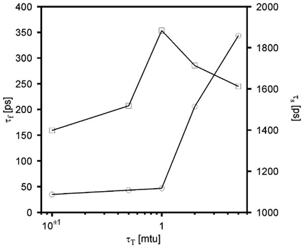
Dependence of the folding (τf, circles) and stability (τs, squares) time on the coupling parameter τT for the Ala10 system obtained in UNRES/MD runs at the temperature T = 300 K with the Berendsen thermostat. Ten 200-ps trajectories were run for each value of τT.
Figure 3.
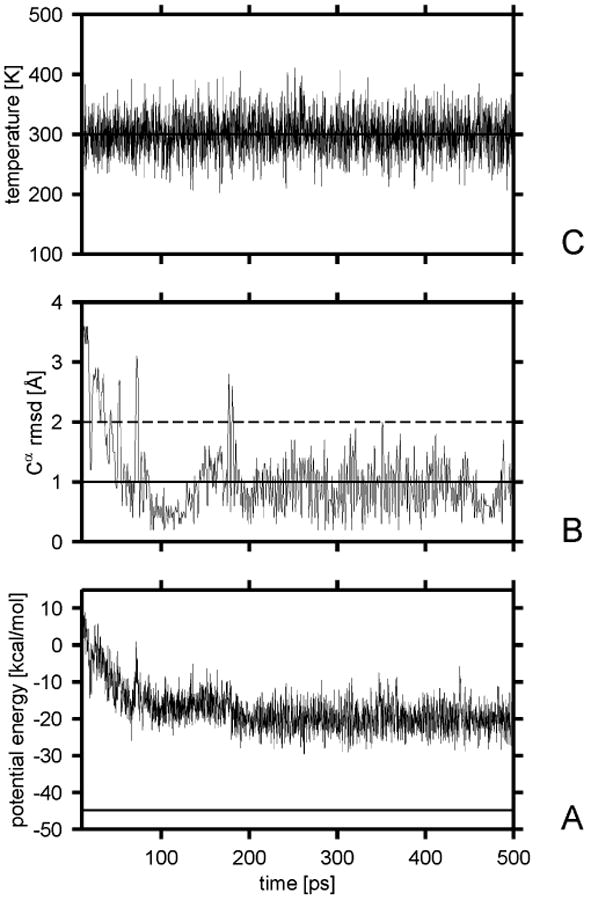
Variation of the potential energy (A), the Cα rmsd from the α-helical structure (B), and the temperature (C) with time for a sample Berendsen trajectory of Ala10 with the UNRES force field obtained with τT = 1 mtu. The solid horizontal line in part A is the lowest potential energy found by the CSA method. The solid horizontal line in panel B corresponds to the 1-Å cutoff of the rmsd over ; after this value was reached, the chain was considered to have folded. The dashed horizontal line in panel B corresponds to the 2-Å rmsd cutoff above which a structure is considered to have left the native basin.
It can be seen (Figure 2) that τf increases rapidly with τT after τT = 1 mtu and decreases slowly with τT for smaller τT. It can, therefore, be concluded that the coupling is too weak for τT > 1 mtu for the system to fold quickly because of too slow exchange of the potential energy with the environment. The stability time varies with τT in the opposite direction, decreasing significantly below τT = 1 mtu. The decrease of the stability time for smaller times is caused by too pronounced coupling to the heat bath and, consequently, too large fluctuations of the potential energy. Therefore, the value of τT at 1 mtu (0.0489 ps) appears to be the optimal one, and we used it in further simulations reported in this paper.
To estimate the plausible values of the scaling factor of the friction coefficient in Langevin simulations, we ran the folding simulations of Ala10 with various scaling factors. By carrying out a similar analysis as for the Berendsen-type simulations, we found that the safe values of the scaling factor for the time step of 0.1 mtu (4.89 fs) range from 0.01 to 0.20. For smaller and higher values, the average temperature starts to deviate by more than 5 K from To, the value specified in the simulation. This is understandable because, with low friction coefficients, the coupling is too weak (as with too large τT values in Berendsen-type simulations), while too large friction results in instability of the integration algorithm because of too large friction forces.27 Sample plots of the potential energy, temperature, and ρα for a representative trajectory corresponding to τT = 1 mtu are shown in Figure 4.
Figure 4.
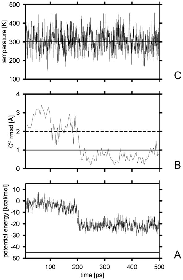
Variation of the potential energy (A), the Cα rmsd from the α-helical structure (B), and the temperature (C) for a sample Langevin trajectory of Ala10 with the UNRES force field obtained with the scaling factor of the friction coefficients of α = 0.05. The solid horizontal line in part A is the lowest potential energy found by the CSA method. The solid horizontal line in panel B corresponds to the 1-Å cutoff of the rmsd over ; after this value was reached, the chain was considered to have folded. The dashed horizontal line in panel B corresponds to the 2-Å rmsd cutoff above which a structure is considered to have left the native basin.
Figure 5 shows the dependence of the folding time on the scaling factor of the friction coefficient. It can be seen that the folding time stays between 200 and 400 ps until the scaling factor reaches 0.1, then the folding time starts to grow approximately linearly with the scaling factor, as observed by Cieplak and co-workers.27,49 It should be noted that, for each α, τf and τs sum up to about 4.9 ns (the length of the simulation). This means that the peptide stays folded after it folds for the first time, as opposed to the results of Berendsen-bath simulations (Figure 2). It should be noted (Table 1) that the average folding time (411 ps) is greater than for simulations with the Berendsen thermostat (52 ps), which is caused by the explicit presence of the friction forces opposing folding.
Figure 5.
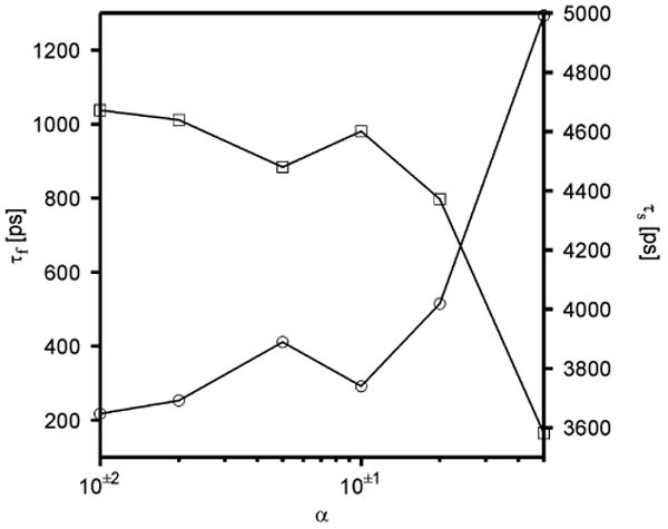
Dependence of the folding time (τf, circles) and stability time (τs, squares) of Ala10 in UNRES Langevin simulations on the scaling factor of the friction coefficients (α of eq 6).
TABLE 1. Folding (τf) and Relative Stability (τs/t)a Times for the Unblocked Ala10 Polypeptide Run with the All-Atom Simulations with Explicit Solvent (7 trajectories), UNRES with Langevin Dynamics (10 trajectories),b the All-Atom Simulations with Implicit Solvent and the Berendsen Thermostat (10 trajectories; τT = 0.1 ps), and UNRES Dynamics with the Berendsen Thermostat (10 trajectories; τT = 1 mtu).
| τf (ps) | τs/t (ps) | |||||
|---|---|---|---|---|---|---|
| force field | min | max | average | max | min | average |
| AMBER explicit water | 1107.0 | 2730.0 | 1748.7 | 0.14 | 0.02 | 0.16 |
| UNRES/Langevin | 19.6 | 1281.2 | 411.2 | 0.99 | 0.74 | 0.92 |
| AMBER GBSA | 8.0 | 670.0 | 200.2 | 0.67 | 0.35 | 0.47 |
| UNRES/Berendsen | 8.8 | 125.2 | 52.5 | 0.95 | 0.57 | 0.77 |
t is the total length of a trajectory.
The friction coefficients were scaled by the factor of 0.05.
3.2. Relationship between the UNRES Time Scale and the Time Scale of All-Atom Molecular Dynamics
As established in the accompanying paper,1 the safe value of the time step (δt) in integrating the equations of motion for microcanonical simulations is 0.02 mtu with a fixed time step or 0.05 mtu with a variable time step; for canonical simulations, the time step can be increased to 0.10 mtu. Even this larger time step corresponds to about 5 fs. However, because fast motions of the secondary degrees of freedom are averaged out in UNRES, it is certain that the time scale of molecular dynamics with UNRES is longer than that of all-atom molecular dynamics.
To estimate the relationship between the time scale of all-atom molecular dynamics and the time scale of molecular dynamics with UNRES, we carried out two series of folding simulations on the Ala10 polypeptide using all-atom dynamics with the AMBER 99 force field39,40 and with UNRES dynamics. The all-atom simulations were carried out with both explicit and implicit solvent for 2 ns. Ten independent trajectories were run for implicit solvent simulations and seven for the simulations with explicit water molecules. The simulations run with explicit solvent were compared with the UNRES Langevin dynamics simulations (in both cases the friction is present either by inclusion of explicit solvent molecules or by considering friction forces), while the all-atom GBSA simulations were compared with UNRES simulations with the Berendsen thermostat (no explicit friction forces being present in both cases). To provide a fair comparison when all-atom GBSA is used, we determined the optimal folding temperature and τT value in all-atom simulations with implicit solvent. These were T = 400 K and τT = 0.1 ps, respectively. The temperature was 300 K in both UNRES Langevin and Berendsen thermostat simulations. We set the scaling factor of the friction coefficient at 0.05 in UNRES Langevin simulations; this value appears in the interval where the folding time varies little with the friction coefficient (Figure 5).
Snapshots from representative all-atom simulations with explicit solvent, with solvent treated at the GBSA level, and UNRES (Langevin and Berendsen) trajectories are shown in Figures 6A–D. The maximum, minimum, and average values of τf and τs for all four approaches are summarized in Table 1. It can be seen that Ala10 folds to the α-helical conformation after about 1.8 ns of all-atom simulations with explicit water and about 0.4 ns of UNRES Langevin simulations on average. Similarly, all-atom implicit solvent simulations required about 0.2 ns on average, while UNRES/MD with the Berendsen thermostat required about 0.05 ns on average. This suggests that the unit of the time step of UNRES dynamics corresponds to about 4 units of all-atom molecular dynamics with explicit solvent. As mentioned in the accompanying paper,1 this is a result of averaging out the fast-moving degrees of freedom when passing to the UNRES from the all-atom representation. The mismatch between the UNRES and all-atom time scales can also be linked to the internal friction,26 which has long been known in polymer physics. The presence of internal friction slows down the internal motion of a polymer chain more than expected based on the viscosity of the surrounding solvent. Part of internal friction is present even when a polypeptide chain is modeled on the all-atom level and the solvent on the mean-field level, because the forces acting on a polymer chain in a solvent cannot be neatly separated into the conservative forces acting within the polypeptide chain and the dissipative forces arising from the bulk of the solvent.50 However, when the motions of an all-atom chain and an UNRES chain are compared, the main difference is likely to arise from the fact that the secondary degrees of freedom (not considered in UNRES) move faster than the coarse-grain (UNRES) degrees of freedom. The coupling of the fast motions to the slow motions of the UNRES degrees of freedom caused the latter to acquire a quasi-random component. (We should bear in mind that an “UNRES chain” physically corresponds to a collection of all-atom chains with the same coarse-grain geometry and velocities of the UNRES sites.) This coupling will, therefore, slow the net motion of the coarse-grain degrees of freedom. As stated in the accompanying paper,1 the coupling of the motion of the secondary to that of the primary degrees of freedom is not taken into account in our present approach, which explains the observed mismatch between the UNRES and the all-atom time scales.
Figure 6.
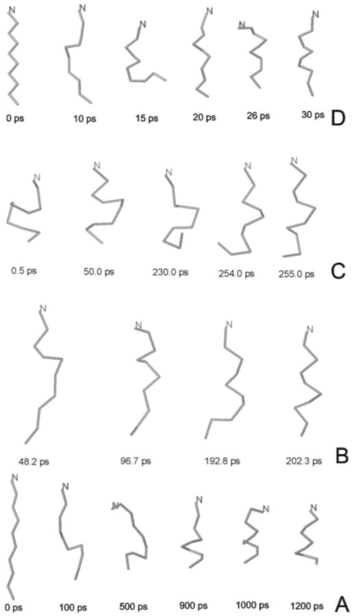
Snapshots from the AMBER all-atom simulations with explicit water molecules (A) compared with Langevin UNRES with α = 0.05 (B), and AMBER all-atom simulations with implicit water (C) compared with Berendsen UNRES (D). The trajectories of the Ala10 polypeptide are shown as α-carbon traces.
Even more favorable is the ratio of the computer time required to fold the Ala10 polypeptide with the all-atom and the UNRES representations: 1 ns of all-atom folding simulations (necessary to fold Ala10) required 10 000 CPU min per single Alpha processor with explicit water molecules and 150 CPU min with implicit solvent. In contrast to this, 1 ns of UNRES simulations (both Langevin and Berendsen) takes 9.3 CPU min. Because, as demonstrated earlier in this section, the UNRES time scale is 4-fold longer than the all-atom time scale, this means that molecular dynamics simulations with the UNRES force field (which is based fully on the physics of interactions in proteins) offer a 4 × (10 000/9.3) ≈ 4000-fold and 4 × (152/9.3) ≈ 65-fold speedup relative to the all-atom MD simulations with explicit and implicit solvent, respectively. Therefore, microsecond if not millisecond times now seem to be within reach.
3.3. Simulations of the Folding of the 46-Residue N-Terminal Fragment of the B-Domain of Staphylococcal Protein A
The Ala10 system is a good test case because computations in real time can be run even in the all-atom scheme with explicit water molecules. However, we are able to study only secondary-structure formation for this decapeptide. Assembling larger fragments rather than formation of secondary structure is a bottleneck of the folding process. We, therefore, ran canonical simulations on protein A, a 46-residue system. Recent work of Jang et al.17 demonstrated that this system folds using an all-atom approach with implicit solvent. We, therefore, studied protein A at both the all-atom (AMBER 99 + GBSA) and the UNRES levels, the UNRES simulations being carried out with both the Berendsen thermostat and the Langevin dynamics.
Jang et al.17 carried out their runs at 400 K and claimed that this temperature was above the folding temperature of the system. We do not share their view for a number of reasons. First, the Berendsen thermostat was used by Jang et al.17 rather than the regular Langevin approach. The stochastic forces that are supposed to kick the system out of a low-energy region in which it is stuck were present only in an implicit manner through temperature scaling. The resulting equations are in fact deterministic, and the stochastic factor is introduced only once when generating the initial velocities. It is, therefore, not clear that a given temperature will correspond to the forces due to the kicks from the solvent molecules characteristic of that temperature. Second, the energy scale of a force field might be different from the physical energy scale. This is especially true for UNRES, which, in its present version, was ultimately optimized to maximize the energy gaps between the conformations with increasing degree of native likeness.14 No information from folding thermodynamics has yet been introduced in optimization except that the initial parameters of the potential of side-chain interactions (USCiSCj) were scaled3 to reproduce the partition coefficients of the amino acids between water and n-octanol.51 However, this constraint was not retained in the optimization of the force field. We, therefore, determined the folding temperature of protein A as a temperature with minimum τf for both the all-atom and the UNRES simulations. We ran five all-atom trajectories and 10 UNRES trajectories per temperature. The settings of the all-atom simulations are described in section 2.4, while, for UNRES, δt = 0.10 mtu (4.89 fs), τT = 1.0 mtu (0.0489 ps), and the duration of a run was 20 ns.
We defined τf and τs as in section 3.1. For UNRES, we used the F2 force field of ref 15; with this force field, the lowest-energy structure of protein A has a 3.2 Å rmsd from the experimental structure (PDB code: 1BDD46). The rmsd was computed from all Cα atoms of the experimental structure of protein A, and the rmsd cutoff to consider a structure folded was 4 Å; the structure was considered to remain in the native basin if the rmsd did not exceed 5 Å.
The plots of the folding and stability versus temperature for both all-atom and UNRES runs are shown in Figure 7. It can be seen that the folding temperature is 420 K for the all-atom (Figure 7B) and 500 K for the UNRES (Figure 7A) approach. Plots of the potential energy, temperature, and rmsd for a representative UNRES trajectory with the Berendsen thermostat at the folding temperature are shown in Figure 8, while snapshots from a representative UNRES trajectory are shown in Figure 9. The corresponding plots obtained in UNRES Langevin dynamics at 500 K with the 0.05 scaling factor of the friction forces are shown in Figures 10 and 11, respectively. The average folding time over 10 trajectories is 4.2 ns for UNRES Langevin dynamics simulations. It can be seen that, regardless of the mode of simulation, the C-terminal α-helix is formed first as found in recent theoretical simulations52–54 and which also is in agreement with experimental studies of the relative stability of helices.55,56 The C-terminal α-helix appears stable throughout a trajectory. It should be noted, though, that earlier theoretical simulations57 suggested that the N-terminal and the middle α-helices are formed first and recent analysis of experimental Φ values suggests that the C-terminal α-helix is poorly formed in the transition state and that the folding starts from the middle α-helix.58 The difference between Berendsen and Langevin simulations is that, in the latter, packing of helices occurs more slowly; this is an explicit effect of introducing friction, which opposes motion more as the larger parts of a polymer chain move simultaneously in a given direction.26
Figure 7.
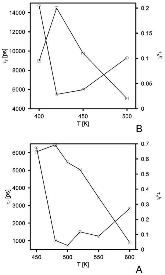
Dependence of the folding (τf, circles) and stability (τs, squares) time for protein A on the temperature in UNRES simulations with the Berendsen thermostat (A) and all-atom AMBER simulations with implicit water modeled at the GBSA level (B). In the all-atom simulations, 5 20-ns trajectories were run, and 10 20-ns trajectories in the UNRES simulations with the Berendsen thermostat. All trajectories were started from fully extended structures.
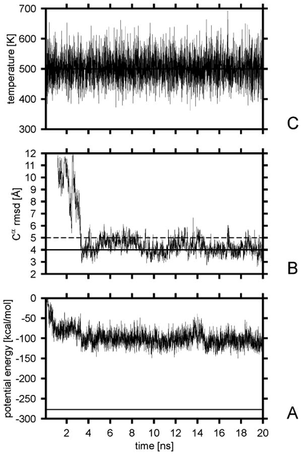
Figure 8.

Variation of the potential energy (A), the Cα rmsd from the native structure (B), and the temperature (C) with time for a sample trajectory of protein A with the UNRES force field and Berendsen thermostat at the folding temperature. The solid horizontal line in part A is the lowest potential energy found in our earlier study14 by the CSA method. The solid horizontal line in panel B corresponds to the 4-Å Cα rmsd cutoff; after reaching this value, the chain was considered to have folded. The dashed horizontal line in panel B corresponds to the 5-Å rmsd cutoff above which a structure is considered to have left the native basin.
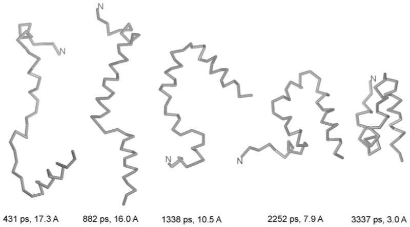
Figure 9.
Snapshots from a representative folding trajectory of protein A at 500 K obtained with the UNRES force field and Berendsen thermostat.
Figure 10.
Variation of the potential energy (A), the Cα rmsd from the native structure (B), and the temperature (C) with time for a sample Langevin trajectory of protein A with the UNRES force field at the folding temperature. The solid horizontal line in part A is the lowest potential energy found in our earlier study14 by the CSA method. The solid horizontal line in panel B corresponds to the 4-Å Cα rmsd cutoff; after reaching this value, the chain was considered to have folded. The dashed horizontal line in panel B corresponds to the 5-Å rmsd cutoff above which a structure is considered to have left the native basin.
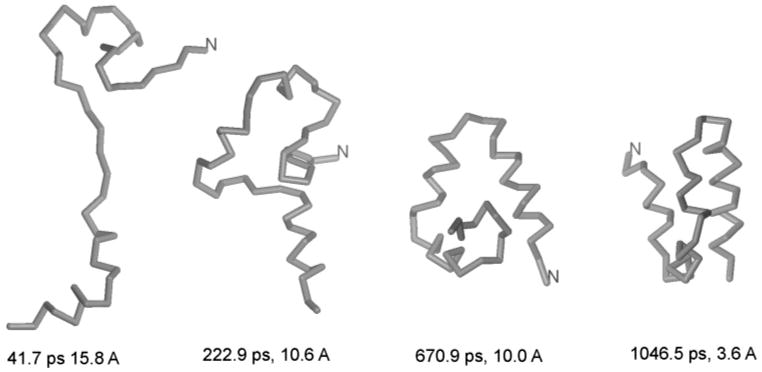
Figure 11.
Snapshots from a representative Langevin folding trajectory of protein A at 500 K obtained with the UNRES force field.
It can be seen in Figure 8B that the molecule folds and unfolds several times during a 20-ns run in the UNRES Berendsen simulations. The average folding time at the folding temperature (τf = 0.74 ns; Figure 7A) is 7.4 times shorter for UNRES (with the Berendsen thermostat) compared to the all-atom simulations with implicit solvent (τf = 5.5 ns; Figure 7B); this ratio is similar to that derived from Ala10 simulations. The average folding time obtained in Langevin simulations (4.2 ns) is longer than that obtained in Berendsen simulations (0.74 ns). Thus, as for Ala10, the presence of explicit friction forces slows down the folding. The average CPU time to fold protein A at 420 K with the all-atom approach is 9136 min/processor (152 h/processor), while that for UNRES (with the Berendsen thermostat) is 30 min/processor. This offers a 305-fold speedup. The time step used in UNRES simulations of protein A (4.89 fs) was larger than that used in the corresponding all-atom simulations (2 fs); it should be noted however that, even when the same time step was used for UNRES as for all-atom dynamics, UNRES still offers about a 100-fold speedup.
It can be seen from Figure 8 that the lowest potential energy obtained during MD runs at the folding temperature is by about 120 kcal/mol higher than the lowest potential energy found in CSA runs. This also occurred for the Ala10 polypeptide, but the difference was smaller because of the smaller size of the system. This suggests that the UNRES force field optimized for protein-structure prediction based on a global-minimum search need not necessarily be good for molecular dynamics, and reoptimization based on MD rather than CSA-generated ensembles is required.
Because the purpose of this study was to perform initial tests of the UNRES/MD approach and to compare the all-atom and the UNRES time scales, we will refrain from further analysis of the folding trajectories here. The all-atom results for protein A will be reported in detail in a separate paper.59 More tests of the UNRES/MD approach on a larger number of proteins have appeared in a separate paper.60
It should be noted that UNRES molecular dynamics can be extended to calculate all-atom folding pathways. The coarse-grained structures from selected points of the pathway can be converted into an all-atom representation using the energy-based method developed in our laboratory,61,62 and limited all-atom MD simulations can subsequently be carried out for each of them. The milestoning method developed recently by Faradjian and Elber63 appears to be very appropriate for the last task.
4. Conclusions
We extended the Lagrange equations for the UNRES model of the polypeptide chain derived in the accompanying paper1 to treat canonical ensembles. We implemented both the Langevin equation with explicit inclusion of the friction and stochastic forces and the Berendsen thermostat in which the friction and stochastic forces are included implicitly. We noted that, owing to the coupling to the thermal bath, which partially removes the energy drift caused by the error inherent in numerical integration, the time step can be increased to 0.1 mtu (4.89 fs), compared to 0.03 mtu (1.494 fs) for the microcanonical mode.1 Comparison of the folding times for the Ala10 polypeptide (obtained with the AMBER 99 force field and explicit water molecules and with the AMBER 99 force field and implicit water treated at the GBSA level) with those obtained with the UNRES Langevin and UNRES Berendsen dynamics, respectively, reveals that the ratio of the UNRES to the all-atom time step is on the order of 4. A 1:7 ratio was obtained when comparing the folding times of protein A (with a three-helix bundle in the native structure) obtained from all-atom simulations with implicit solvent and UNRES simulations with the Berendsen thermostat. The dependence of the ratio of the UNRES to all-atom time scale on the system suggests that the effect of averaging out the internal degrees of freedom (the internal friction26) is system-dependent, and the equations of motion must be derived rigorously to establish the relationship between the UNRES and the all-atom and, ultimately, between the UNRES and the experimental time scales (not just based on the folding events as is done in this work). This can probably be accomplished by using the perturbation theory developed by van Kampen.64 Research in this direction is currently underway in our laboratory.
Simulations of protein A have also demonstrated that molecular dynamics with UNRES is applicable to folding proteins and not only model polypeptides, using both the Berendsen thermostat and the full-blown Langevin dynamics. Simulations with the Berendsen thermostat result in quicker folding but are less realistic compared to Langevin dynamics simulations because of the absence of explicit friction in the former. Analysis of the CPU times required for folding demonstrates that UNRES offers at least a 4000-fold speedup relative to the all-atom approach with explicit water molecules and a 65-fold speedup relative to the all-atom approach with implicit water; the folding time of protein A using the Berendsen thermostat is 30 min on a single Alpha processor compared to about 152 h required for all-atom simulations with implicit solvent. This enables us to target a microsecond, if not a millisecond, time scale for protein folding.
It is interesting to note that, based on the experimental values of the folding times of α-helices, which are of the order of 0.6 μs,65 one can conclude that both all-atom and UNRES time scales are underestimated. Even taking into account the fact that Ala10 is a faster folder than the model helical peptides used to estimate helix folding rates from experiment,65 the time for folding this peptide should amount to at least 100 ns while, even with the all-atom approach with explicit water molecules, we obtained a 1-ns folding time. The answer to this is rather simple: Even when the solvent is treated at the detailed atomistic level, the vibrations of its bonds are suppressed by the SHAKE algorithm.42,43 Without doing this, one observes primarily only collective vibrations of the solvent molecules, while the solute molecule remains highly intact. This means that a large part of the fast motions are removed by SHAKE even when the detailed approach is used. For protein A, the average folding time with UNRES dynamics was 4.5 ns, while the shortest folding times measured experimentally are on the order of microseconds even for very fast folding proteins.65 Consequently, a unit of the UNRES time step corresponds to about 1000 units of the physical time scale.
It could be suspected that the short folding times obtained in our study are caused by the fact that UNRES is biased toward reproducing folded states relative to unfolded ones, because part of this force field consists of statistical potentials derived from the PDB. It should be noted, however, that the early versions of UNRES in which the bulk of the force field consisted of statistical potentials2–4 were not capable of ab initio folding and required constraining the virtual-bond angles at 90° 2 or were only good for threading.3,4 The capability of spontaneous secondary-structure formation and, thereby, ab initio folding was achieved only after the cumulant-based correlation terms were introduced.5,7,13 These terms do not contain any information from the PDB statistics, are entirely physics-based, and were parametrized using ab initio quantum-mechanical energy surfaces of model systems.13 The force field used in this work was ultimately parametrized by hierarchical optimization using 1IGD as a training protein; however, this is an α + β protein as opposed to protein A studied in this work, which is an α protein. Thus, the force field is biased toward the native structure of 1IGD but not protein A. An interesting fact is that, although the force field was parametrized using 1IGD (but energy-minimized and not with MD decoys), MD simulations of this protein result in non-native structures, although the nativelike structure is the global minimum in the potential-energy surface.60 The reason for this is the neglect of a large portion of configurational entropy when using energy-minimized decoys, while full configurational entropy is present in MD. Therefore, structures higher in energy but occupying a larger portion of conformational space will dominate in MD, while they will be rejected when using a global optimizer based on the potential energy as a scoring function.60 Therefore, the fact that decoys from energy minimization and not from MD simulations were used in parametrization is a disadvantage as far as attraction toward native structure in MD simulations is concerned.
Acknowledgments
We are indebted to Dr. Paweł Grochowski and Professor Bogdan Lesyng, University of Warsaw, for valuable suggestions and comments on the manuscript. This work was supported by grants from the National Institutes of Health (NIH) (GM-14312), the National Science Foundation (MCB00-03722), the NIH Fogarty International Center (TW1064), and the Polish Ministry of Scientific Research and Information Technology (3 T09A 032 26 and 6 T11 2003 C/06098). This research was conducted by using the resources of (a) our 392-processor Beowulf cluster at the Baker Laboratory of Chemistry and Chemical Biology, Cornell University, (b) the National Science Foundation Terascale Computing System at the Pittsburgh Supercomputer Center, (c) our 45-processor Beowulf cluster at the Faculty of Chemistry, University of Gdańsk, (d) the Informatics Center of the Metropolitan Academic Network in Gdańsk, and (e) the Interdisciplinary Center of Mathematical and Computer Modelling at the University of Warsaw.
Appendix: Adaptation of the Integration Algorithm from TINKER to Molecular Dynamics with UNRES
Let us transform eq 3 to a system of equations with a diagonal friction matrix. For this purpose, we first introduce new variables z related to q by eq A1.
| (A1) |
The Langevin equations can now be written as eq A2.
| (A2) |
with
| (A3) |
| (A4) |
| (A5) |
Now, by definition of the new variables
| (A6) |
where V is the matrix of the eigenvectors of T, we can transform eq A2 to a system of uncoupled differential equations
| (A7) |
where τi is the ith eigenvalue of matrix T.
The stochastic integrator developed in refs 32 and 33 can now be implemented to eq A7, and the new quantities ξ and ξ̇ can be transformed back to the original space. Steps 1 and 2 of the stochastic velocity Verlet algorithm are now the following:
Step 1:
| (A8) |
Step 2:
| (A9) |
with
| (A10) |
| (A11) |
| (A12) |
| (A13) |
| (A14) |
| (A15) |
where s, t, u, w, x, and y are diagonal matrices with the diagonal elements defined by eqs A16–A21, respectively.
| (A16) |
| (A17) |
| (A18) |
| (A19) |
| (A20) |
| (A21) |
with
| (A22) |
| (A23) |
| (A24) |
This algorithm is more expensive compared to the simplified stochastic velocity Verlet algorithm described in section 2.2 because of the need to perform many matrix multiplications and to diagonalize the ATΓA matrix, if the friction coefficients (which depend on solvent-accessible surface area and, consequently, on conformation) are evaluated frequently. The last feature was not a big issue in our study, because we evaluate the friction coefficients only every 1000 MD steps. However, 7 multiplications of vectors by matrices must be carried out at each integration step, compared to 3 when applying the simplified algorithms (in the latter case those involve computation of the friction forces and the computation of accelerations from forces). Moreover, with our variable-time-step algorithm described in the accompanying paper,1 the matrices S, T, U, W, X, and Y must be reevaluated every time the time step is changed; this involves 12 matrix multiplications. We reduced this cost by storing the matrices for each time step, because the time step in our algorithm is always scaled down by integer powers of 2 (eq 42 of ref 1). By carrying out test calculations, we found that, given the values of the time step and the friction coefficients used in this study, the factors are approximately and the matrices S, T, U, W, X, and Y are almost diagonal. With the additional assumption that the correlation coefficients ρ between velocities and positions are almost equal to zero, the TINKER algorithm reduces to the simplified stochastic velocity Verlet algorithm described in section 2.2. Consequently, we used the simplified algorithm in all tests reported in the paper.
We also adapted the stochastic integrator introduced by Ciccotti and co-workers36,37 to the Langevin equations for UNRES. The derivation of the pertinent equations is similar to those for TINKER.
References and Notes
- 1.Khalili M, Liwo A, Rakowski F, Grochowski P, Scheraga HA. J Phys Chem B. 2005;109:13785. doi: 10.1021/jp058008o. [DOI] [PMC free article] [PubMed] [Google Scholar]
- 2.Liwo A, Pincus MR, Wawak RJ, Rackovsky S, Scheraga HA. Protein Sci. 1993;2:1715. doi: 10.1002/pro.5560021016. [DOI] [PMC free article] [PubMed] [Google Scholar]
- 3.Liwo A, Ołdziej S, Pincus MR, Wawak RJ, Rackovsky S, Scheraga HA. J Comput Chem. 1997;18:849. [Google Scholar]
- 4.Liwo A, Pincus MR, Wawak RJ, Rackovsky S, Ołdziej S, Scheraga HA. J Comput Chem. 1997;18:874. [Google Scholar]
- 5.Liwo A, Kaźmierkiewicz R, Czaplewski C, Groth M, Ołdziej S, Wawak RJ, Rackovsky S, Pincus MR, Scheraga HA. J Comput Chem. 1998;19:259. [Google Scholar]
- 6.Liwo A, Lee J, Ripoll DR, Pillardy J, Scheraga HA. Proc Natl Acad Sci USA. 1999;96:5482. doi: 10.1073/pnas.96.10.5482. [DOI] [PMC free article] [PubMed] [Google Scholar]
- 7.Liwo A, Czaplewski C, Pillardy J, Scheraga HA. J Chem Phys. 2001;115:2323. [Google Scholar]
- 8.Lee J, Ripoll DR, Czaplewski C, Pillardy J, Wedemeyer WJ, Scheraga HA. J Phys Chem B. 2001;105:7291. [Google Scholar]
- 9.Pillardy J, Czaplewski C, Liwo A, Wedemeyer WJ, Lee J, Ripoll DR, Arłukowicz P, Ołdziej S, Arnautova YA, Scheraga HA. J Phys Chem B. 2001;105:7299. [Google Scholar]
- 10.Pillardy J, Czaplewski C, Liwo A, Lee J, Ripoll DR, Kaźmierkiewicz R, Ołdziej S, Wedemeyer WJ, Gibson KD, Arnautova YA, Saunders J, Ye YJ, Scheraga HA. Proc Natl Acad Sci USA. 2001;98:2329. doi: 10.1073/pnas.041609598. [DOI] [PMC free article] [PubMed] [Google Scholar]
- 11.Liwo A, Arłukowicz P, Czaplewski C, Ołdziej S, Pillardy J, Scheraga HA. Proc Natl Acad Sci USA. 2002;99:1937. doi: 10.1073/pnas.032675399. [DOI] [PMC free article] [PubMed] [Google Scholar]
- 12.Ołdziej S, Kozłowska U, Liwo A, Scheraga HA. J Phys Chem A. 2003;107:8035. [Google Scholar]
- 13.Liwo A, Ołdziej S, Czaplewski C, Kozłowska U, Scheraga HA. J Phys Chem B. 2004;108:9421. [Google Scholar]
- 14.Liwo A, Arłukowicz P, Ołdziej S, Czaplewski C, Makowski M, Scheraga HA. J Phys Chem B. 2004;108:16918. [Google Scholar]
- 15.Ołdziej S, Liwo A, Czaplewski C, Pillardy J, Scheraga HA. J Phys Chem B. 2004;108:16934. [Google Scholar]
- 16.Ołdziej S, Ła̧giewka J, Liwo A, Czaplewski C, Chinchio M, Nanias M, Scheraga HA. J Phys Chem B. 2004;108:16950. [Google Scholar]
- 17.Jang S, Kim E, Shin S, Pak Y. J Am Chem Soc. 2003;125:14841. doi: 10.1021/ja034701i. [DOI] [PubMed] [Google Scholar]
- 18.Levy RM, Karplus M, McCammon JA. Chem Phys Lett. 1979;65:4. [Google Scholar]
- 19.Yun-Yu S, Lu W, van Gunsteren WF. Mol Simul. 1988;1:369. [Google Scholar]
- 20.Levitt M. J Mol Biol. 1976;104:59. doi: 10.1016/0022-2836(76)90004-8. [DOI] [PubMed] [Google Scholar]
- 21.Richmond TJ. J Mol Biol. 1984;178:63. doi: 10.1016/0022-2836(84)90231-6. [DOI] [PubMed] [Google Scholar]
- 22.Wesson L, Eisenberg D. Protein Sci. 1992;1:227. doi: 10.1002/pro.5560010204. [DOI] [PMC free article] [PubMed] [Google Scholar]
- 23.http://dasher.wustl.edu/tinker/.
- 24.Ren P, Ponder JW. J Phys Chem B. 2003;107:5933. [Google Scholar]
- 25.Veitshans T, Klimov D, Thirumalai D. Folding Des. 1996;2:1. doi: 10.1016/S1359-0278(97)00002-3. [DOI] [PubMed] [Google Scholar]
- 26.de Gennes PG. Scaling Concepts in Polymer Physics. Chapter VI Cornell University Press; Ithaca, NY: 1979. [Google Scholar]
- 27.Cieplak M, Hoang TX, Robbins MO. Proteins: Struct, Funct, Genet. 2002;49:104. doi: 10.1002/prot.10188. [DOI] [PubMed] [Google Scholar]
- 28.van Gunsteren WF, Berendsen HJC. Mol Phys. 1982;45:637. [Google Scholar]
- 29.van Gunsteren WF, Berendsen HJC. Mol Simul. 1988;1:173. [Google Scholar]
- 30.van Gunsteren WF. Molecular dynamics and stochastic dynamics: A primer. In: van Gunsteren WF, Weiner PK, Wilkinson AJ, editors. Computer Simulation of Biomolecular Systems. ESCOM; Leiden, The Netherlands: 1993. pp. 3–36. [Google Scholar]
- 31.Zhang G, Schlick T. Mol Phys. 1995;84:1077. [Google Scholar]
- 32.Allen MP. Mol Phys. 1980;40:1073. [Google Scholar]
- 33.Guarnieri F, Still WC. J Comput Chem. 1994;15:1302. [Google Scholar]
- 34.Paterlini MG, Ferguson DM. Chem Phys. 1998;236:243. [Google Scholar]
- 35.Suzuki M. Proc Jpn Acad, Ser B. 1993;69:161. [Google Scholar]
- 36.Ricci A, Ciccotti G. Mol Phys. 2003;101:1927. [Google Scholar]
- 37.Ciccotti G, Kalibaeva G. Philos Trans R Soc London, Ser A. 2004;362:1583. doi: 10.1098/rsta.2004.1400. [DOI] [PubMed] [Google Scholar]
- 38.Berendsen HJC, Postma JPM, van Gunsteren WF, DiNola A, Haak JR. J Chem Phys. 1984;81:3684. [Google Scholar]
- 39.Weiner SJ, Kollman PA, Nguyen DT, Case DA. J Comput Chem. 1986;7:230. doi: 10.1002/jcc.540070216. [DOI] [PubMed] [Google Scholar]
- 40.Pearlman DA, Case DA, Caldwell JW, Ross WS, Cheatham TE, III, DeBolt S, Ferguson D, Seibel G, Kollman P. Comput Phys Commun. 1995;91:11. [Google Scholar]
- 41.Jorgensen WL, Chandrasekhar J, Madura JD, Impey RW, Klein ML. J Chem Phys. 1983;79:926. [Google Scholar]
- 42.Ryckaert JP, Ciccotti G, Berendsen HJC. J Comput Phys. 1977;23:327. [Google Scholar]
- 43.van Gunsteren WF, Berendsen HJC. Mol Phys. 1977;34:1311. [Google Scholar]
- 44.Cramer CJ, Truhlar DG. Chem Rev. 1999;99:2161. doi: 10.1021/cr960149m. [DOI] [PubMed] [Google Scholar]
- 45.Bashford D, Case DA. Annu Rev Phys Chem. 2000;51:129. doi: 10.1146/annurev.physchem.51.1.129. [DOI] [PubMed] [Google Scholar]
- 46.Gouda H, Torigoe H, Saito A, Sato M, Arata Y, Shimada I. Biochemistry. 1992;31:9665. doi: 10.1021/bi00155a020. [DOI] [PubMed] [Google Scholar]
- 47.Némethy G, Gibson KD, Palmer KA, Yoon CN, Paterlini G, Zagari A, Rumsey S, Scheraga HA. J Phys Chem. 1992;96:6472. [Google Scholar]
- 48.Lee J, Liwo A, Scheraga HA. Proc Natl Acad Sci USA. 1999;96:2025. doi: 10.1073/pnas.96.5.2025. [DOI] [PMC free article] [PubMed] [Google Scholar]
- 49.Hoang TX, Cieplak M. J Chem Phys. 2000;112:6851. [Google Scholar]
- 50.Qiu L, Hagen SJ. Chem Phys. 2004;307:243. [Google Scholar]
- 51.Fauchere JL, Pliška V. Eur J Med Chem. 1983;18:369. [Google Scholar]
- 52.Alonso DOV, Daggett V. Proc Natl Acad Sci USA. 2000;97:133. doi: 10.1073/pnas.97.1.133. [DOI] [PMC free article] [PubMed] [Google Scholar]
- 53.Takada S. Proteins: Struct, Funct, Genet. 2001;42:85. [Google Scholar]
- 54.Ghosh A, Elber R, Scheraga HA. Proc Natl Acad Sci USA. 2002;99:10394. doi: 10.1073/pnas.142288099. [DOI] [PMC free article] [PubMed] [Google Scholar]
- 55.Bottomley SP, Popplewell AG, Scawen M, Wan T, Sutton BJ, Gore MG. Protein Eng. 1994;7:1463. doi: 10.1093/protein/7.12.1463. [DOI] [PubMed] [Google Scholar]
- 56.Bai YW, Karimi A, Dyson HJ, Wright PE. Protein Sci. 1997;6:1449. doi: 10.1002/pro.5560060709. [DOI] [PMC free article] [PubMed] [Google Scholar]
- 57.Guo ZY, Brooks CL, Boczko EM. Proc Natl Acad Sci USA. 1997;94:10161. doi: 10.1073/pnas.94.19.10161. [DOI] [PMC free article] [PubMed] [Google Scholar]
- 58.Sato S, Religa TL, Daggett V, Fersht AR. Proc Natl Acad Sci USA. 2004;101:6952. doi: 10.1073/pnas.0401396101. [DOI] [PMC free article] [PubMed] [Google Scholar]
- 59.Jagielska A, Scheraga HA. manuscript to be submitted for publication. [Google Scholar]
- 60.Liwo A, Khalili M, Scheraga HA. Proc Natl Acad Sci USA. 2005;102:2362. doi: 10.1073/pnas.0408885102. [DOI] [PMC free article] [PubMed] [Google Scholar]
- 61.Kaźmierkiewicz R, Liwo A, Scheraga HA. J Comput Chem. 2002;23:715. doi: 10.1002/jcc.10068. [DOI] [PubMed] [Google Scholar]
- 62.Kaźmierkiewicz R, Liwo A, Scheraga HA. Biophys Chem. 2003;100:261. doi: 10.1016/s0301-4622(02)00285-5. [DOI] [PubMed] [Google Scholar]; Biophys Chem. 2003;106:9. Erratum. [Google Scholar]
- 63.Faradjian AK, Elber R. J Chem Phys. 2004;120:10880. doi: 10.1063/1.1738640. [DOI] [PubMed] [Google Scholar]
- 64.van Kampen CW. Phys Rep. 1985;124:69. [Google Scholar]
- 65.Kubelka J, Hofrichter J, Eaton WA. Curr Opin Struct Biol. 2004;14:76. doi: 10.1016/j.sbi.2004.01.013. [DOI] [PubMed] [Google Scholar]