Model Misspecification: Finite Mixture or Homogeneous?

Abstract

A common problem in statistical modelling is to distinguish between finite mixture distribution and a homogeneous non-mixture distribution. Finite mixture models are widely used in practice and often mixtures of normal densities are indistinguishable from homogenous non-normal densities. This paper illustrates what happens when the EM algorithm for normal mixtures is applied to a distribution that is a homogeneous non-mixture distribution. In particular, a population-based EM algorithm for finite mixtures is introduced and applied directly to density functions instead of sample data. The population-based EM algorithm is used to find finite mixture approximations to common homogeneous distributions. An example regarding the nature of a placebo response in drug treated depressed subjects is used to illustrate ideas.

1 Introduction

A guiding principle in statistical modelling is Occam’s Razor, attributed to William of Ockham (1285–1349), which states that “if two theories explain the facts equally well then the simpler theory is to be preferred.” Figure 1 shows a histogram of the change in the Hamilton Depression scale (HAM-D) from baseline (week 0) to week 1 for depressed individuals treated with Prozac. The differences are mostly positive indicating that most of the subjects have experienced some improvement in mood after only one week on Prozac. However it is generally believed that it takes more than a week before to benefit from the chemical component of the drug. Thus, much of the improvement seen in Figure 1 is likely due to an initial placebo response. Overlaid on the histogram are two density curves: the dashed curve is a density of a mixture with k = 2 normal components (see e.g. Titterington et al., 1985) and the solid curve is a skew-normal density (e.g Azzalini and Capitanio, 1999). Both densities in Figure 1 are very similar to each other and they fit the data quite well. The skew normal density requires three parameters while the 2-component normal mixture requires 5 parameters. According to William of Ockham’s principle, we should prefer the simpler skew-normal model over the more complicated the finite mixture model.

Figure 1.

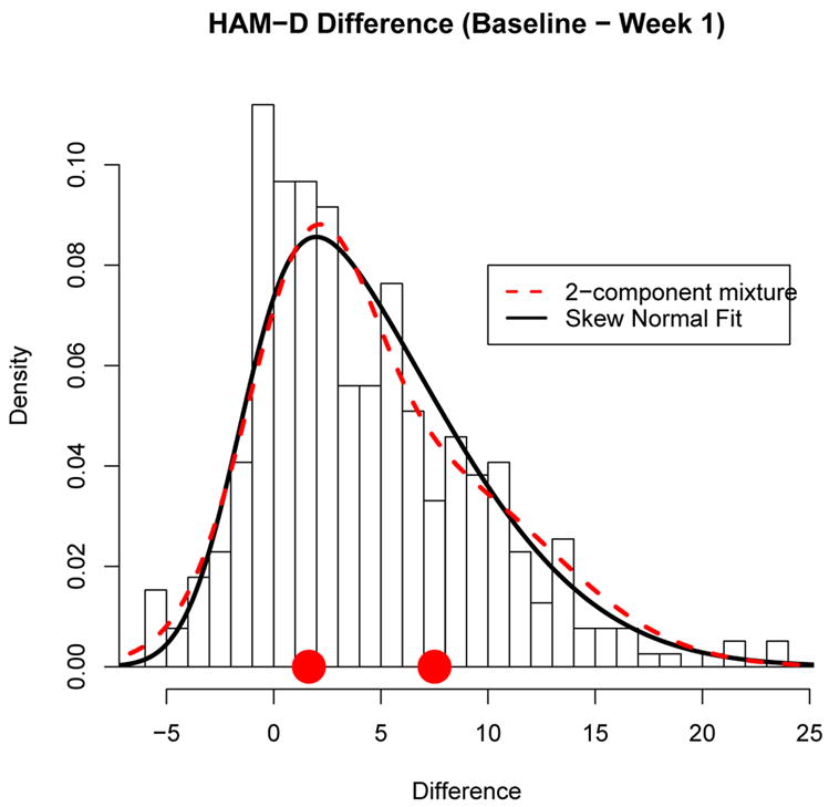
Histogram of HAM-D difference (Baseline – Week 1) showing the amount of improvement in mood after 1 week on Prozac. The solid curve is a skew-normal density and the dashed curve is a 2-component normal finite mixture density. The 2 points on the x-axis are the normal mixture component means.

On the other hand, Murphy claims that “… simplicity is a dangerous ideal” (Murphy, 1964, page 320). Perhaps the guiding principle to statistical modelling should be to employ the model closest to the truth. Thus a more complicated model may be preferred over a simpler model if it is provides a better representation of the truth and can be adequately estimated. However, the truth is infinitely complex and consequently, as George Box pointed out, “all models are wrong, some are useful.” The true model underlying Figure 1 is unknown. The skew normal and the finite mixture models both fit the data well but they offer two competing but different approximations to the truth. If there exist two distinct groups (e.g. those who do and do not experience a placebo response) then the finite mixture model is appropriate. If selection of treatment for depression depends on group membership, then the mixture model can be used to ascertain the group membership. On the other hand, perhaps the placebo effect skews the distribution towards improvement and everyone experiences a placebo response, the degree of which varies over a continuum. If this is the case, then distinct groups do not exist and a treatment program predicated on the existence of distinct groups may be inappropriate. By the way, if the finite mixture model interpretation is correct with one group not experiencing a placebo response in the Prozac example, then one of the mixture component means in the Prozac example should be zero.

The motivation for this paper came from work on distinguishing a placebo response from a drug response in depression studies. Determining the most appropriate statistical analysis of the data depends on whether or not there exist well-defined mixture components (e.g. those who do and do not exhibit a placebo response). In some finite mixture applications, there do exist well-defined mixture components (e.g. males and females). However, in many other examples (such as the Prozac example above), the existence of well-defined mixture components is speculative. The problem, highlighted in this paper, is that in many cases mixture distributions and homogeneous non-normal distributions will be virtually identical to one another. Discerning a finite mixture from some other homogeneous non-normal distribution is an old problem. Pearson (1895) states “The question may be raised, how are we to discriminate between a true curve of skew type and a compound curve,” where by compound he means mixture. Murphy (1964) lists several examples from hypertension to eye and hair color where the existence of distinct groups is unclear and says, “It is one thing to argue from mechanisms to expected outcomes; it is very much more difficult and hazardous to argue from observations back to mechcanisms” (page 312) meaning that it is dangerous to posit the existence of a mixture simply from observed data. Murphy (1964) as well as Titterington et al. 1985 each give an example where a finite normal mixture with k = 2 components can be well approximated by a lognormal distribution and they note that it “can be very difficult to identify the ‘correct’ model. More recently Bauer and Curran (2003) demonstrate that a growth mixture model may appear optimal even in cases where the true distribution is not a mixture.

Bauer and Curran (2003) also note that finite mixture models serve two distinctly different purposes: (i) the mixture components can represent distinct subgroups in the population or (ii) the mixture model may provide an approximation to a non-normal but homogeneous population. In the latter case, interpreting the mixture components as genuine subgroups is erroneous.

Closely related to finite mixture models is clustering (discussed in Section 5). The k-means algorithm (e.g. Forgy, 1965; Hartigan and Wong, 1979; MacQueen, 1967) is frequently used to discover distinct clusters in a data set. If the data is from a homogeneous distribution, the k-means algorithm will nonetheless converge to a set of well-defined cluster means which are called self-consistent points (Flury, 1993) of the empirical distribution and are estimators of the principal points of the underlying distribution (Flury, 1990). This paper deals with the related problem of determining mixture component means when the EM algorithm is applied to a non-mixture.

In order to determine what the EM algorithm is estimating when applied to a non-mixture, a population-based EM algorithm is proposed in Section 2 whereby the EM algorithm is run, not on sample data, but run directly on the underlying density of the distribution. The population-based EM algorithm is illustrated on some common non-normal but homogeneous distributions in Section 3. The population-based EM algorithm is applied to nonparametric density estimators in Section 4. The issue of estimating clusters and mixture components is revisited in Section 5. The paper is concluded in Section 6. The computational results throughout the paper were obtained using the R-software package (R Development Core Team, 2003).

2 A Population-Based EM Algorithm

The density for a k component finite mixture model is defined as

$$f(\mathit{y})=\sum _{j=1}^k{\pi }_j{f}_j(\mathit{y}),$$ (2.1)

where the prior probabilities π_j’s add to one and the f_j’s are the densities of the mixture components. In many applications, the mixture component densities are assumed to be multivariate normal where f_j(y) = N (y; μ_j, Ψ_j) is a p-variate normal density with mean μ_j and covariance Ψ_j.

Given a sample y₁, …, y_n, one seeks the values of the parameters that maximize the log-likelihood

$$l(\mathit{\theta })=\sum _{i=1}^{n}log(f({\mathit{y}}_i;\mathit{\theta })),$$ (2.2)

where θ are the mixture model parameters. The EM algorithm (Dempster et al., 1977) is often used to determine maximum likelihood estimates of the parameters of a finite mixture. The idea is to introduce a multinomial latent indicator variable x that indicates group membership. The “E”-step in the EM algorithm replaces the complete data log-likelihood in terms of (x_i, y_i) by its conditional expectation given the observed data. For finite normal mixtures, the complete log-likelihood is linear in x and thus, the “E”-step in the EM algorithm replaces the unobserved x by its conditional expectation given y which produces (2.3) below. The “M”-step of the EM algorithm then determines the parameter values that maximizes the expected log-likelihood. For the finite mixture of normals, the EM algorithm iterates between the following two steps:

Finite Mixture EM Algorithm for Sample Data

1. (E-step) Set

   $${\pi }_{ji}=\frac{{\pi }_j{f}_j({\mathit{y}}_i)}{f({\mathit{y}}_i)}.$$ (2.3)

2. (M-step): Set

   $${\pi }_j=\frac{1}{n}\sum _{i=1}^n{\pi }_{ji},\hspace{0.17em}\hspace{0.17em}\hspace{0.17em}j=1,\dots ,k.$$ (2.4)

   $${\mathit{\mu }}_j=\frac{1}{n{\pi }_j}\sum _{i=1}^n{\pi }_{ji}{\mathit{y}}_i,j=1,\dots ,k.$$ (2.5)

   $${\mathrm{\Psi }}_j=\frac{1}{n{\pi }_j}\sum _{i=1}^n{\pi }_{ji}({\mathit{y}}_i-{\mathit{\mu }}_j)({\mathit{y}}_i-{\mathit{\mu }}_j{)}^{\prime }.$$ (2.6)

The question of interest is what happens when the EM algorithm for a finite mixture is applied to data that is not from a finite mixture. To answer this question, we consider a population-based version of the EM algorithm. The population version of the log-likelihood in (2.2) is

$$\int f(\mathit{y};\mathit{\theta })log(f(\mathit{y};\mathit{\theta }))d\mathit{y}.$$ (2.7)

Now, suppose the true underlying density is g(y) which differs from f(y; θ) on a set of positive measure. Then the misspecified population-based version of the log-likelihood becomes

$$\int g(\mathit{y})log(f(\mathit{y};\mathit{\theta }))d\mathit{y}.$$ (2.8)

The idea is to maximize this misspecified population-based log-likelihood with respect to θ using a population-based version of the EM algorithm. This maximization can be accomplished using population-based versions of (2.3)–(2.6):

Misspecified Population-Based EM Algorithm

1. (E-step) Define the following posterior probability functions for h = 1, …, k:

$${\pi }_h(\mathit{y})=\frac{{\pi }_h{f}_h(\mathit{y})}{{\sum }_{j=1}^k{\pi }_j{f}_j(\mathit{y})}.$$ (2.9)

1. (M-Step): Set

$$\begin{array}{l}{\pi }_h=\int g(\mathit{y}){\pi }_h(\mathit{y})d\mathit{y}\\ {\mathit{\mu }}_h=\int \mathit{y}g(\mathit{y}){\pi }_h(\mathit{y})d\mathit{y}\\ {\mathbf{\Psi }}_h=\int (\mathit{y}-{\mathit{\mu }}_h)(\mathit{y}-{\mathit{\mu }}_h{)}^{\prime }g(\mathit{y}){\pi }_h(\mathit{y})d\mathit{y}.\end{array}$$

The M-step equations come from maximizing the complete misspecified population-based expected log-likelihood for the finite mixture model with respect to the mixture parameters:

$$\sum _{h=1}^k\int g(\mathit{y}){\pi }_h(\mathit{y})[log({\pi }_h)+log(f_h(\mathit{y}))]d\mathit{y}.$$ (2.10)

Typically numerical integration techniques will be necessary to evaluate the integrals in the M-step above and we have used numerical integration in the examples in this paper. In particular, we have used the integrate function in R (R Development Core Team, 2003) which is an adaptive quadrature method based on Quadpack routines (Piessens et al., 1983). In higher dimensions, one can perform repeated one-dimensional integrals but this approach requires an exponentially increasing number of function evaluations as the dimension increases. Alternatively one can use Monte Carlo integration methods (e.g. Swartz and Evans, 2000) or number theoretic methods (Fang and Wang, 1994). The examples that follow require one and two dimensional integrations.

Beginning with initial parameter values for the finite mixture and iterating the population-based EM algorithm between steps (1) and (2) above will then determine a finite mixture density that approximates a given density g(y). (2.10) is maximized at the “M”-step of the EM algorithm and consequently, the misspecified population-based log-likelihood monotonically increases as the EM algorithm iterates (e.g. see McLachlan and Krishnan, 1997, p. 83).

Replacing the misspecified mixture density f(y) in the logarithm in (2.8) by the correct density g(y) gives the negative of the entropy:

$$\text{Entropy}:-\int g(\mathit{y})log(g(\mathit{y}))d\mathit{y}.$$

Using the following inequality (e.g. Topsøe, 2001, p. 166)

$$xlog\left(\frac{x}{y}\right)=-xlog\left(\frac{y}{x}\right)\ge x-y,$$

it follows that

$$\int g(\mathit{y})log(f(\mathit{y}))d\mathit{y}\le \int g(\mathit{y})log(g(\mathit{y}))d\mathit{y}.$$

That is, the misspecified population-based log-likelihood for the finite mixture model is less than or equal to the true population-based log-likelihood. As the population-based EM algorithm iterates, the difference between the misspecified population-based log-likelihood and the true population-based log-likelihood diminishes.

In general one can choose any continuous density g(y) to use in the misspecified population-based EM algorithm described above. The next section demonstrates the algorithm for some well-known densities (gamma, beta, skew-normal). Given a data set that is clearly non-normal, one can chose a density g(y) from a parametric family that provides a good fit to the data, such as the skew normal density in Figure 1. Alternatively, one can set g(y) equal to a nonparametric density estimate, see Section 4. The population-based EM algorithm can then be applied to the density g(y) to determine if a finite mixture model is also a plausible model for the data.

3 Examples

In this section we apply the population-based EM algorithm to some well-known distributions. We defined convergence of the algorithm to be when the squared difference between the misspecified log-likelihood (2.8) on successive iterations was less than 10⁻¹⁵. In the following examples, we did not put a limit on the number of iterations for the EM algorithm. Instead we allowed the algorithm to iterate until the convergence criterion was met.

3.1 The Normal Distribution

The population-based EM algorithm does not converge when applied to a single normal distribution because the parameters are not identifiable. For example, for k = 2 mixture components, one can obtain identical solutions for any combination of prior probabilities π₁ and π₂ that sum to one. When the population-based EM algorithm is applied to a normal density, it iterates indefinitely.

3.2 The Beta Distribution

The beta distribution with parameters a and b produces a very wide variety of density shapes. Figure 2 shows three distinct beta density curves (solid curves) with parameters a = b = 1 (uniform distribution) in the top panel; a = 2, b = 4 in the middle panel and a = 5, b = 5 in the bottom panel. In each case, the misspecified population-based EM algorithm was run on these beta distributions for k = 2 mixture components.

Figure 2.

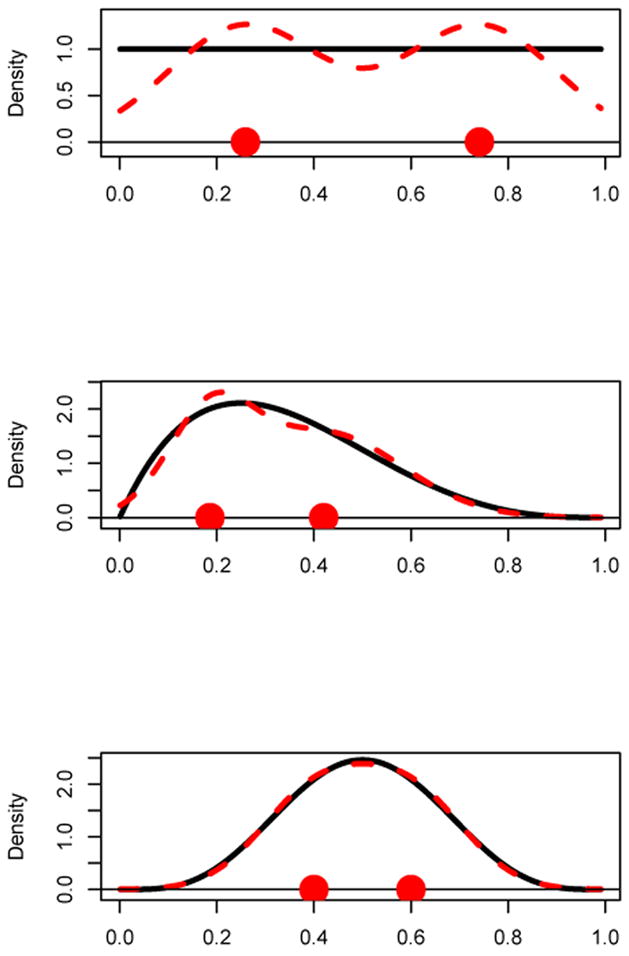
Beta densities and the corresponding best fitting k = 2 component normal mixtures obtained from the population-based EM algorithm. Top Panel: a = b = 1 (uniform distribution); Middle Panel: a = 2, b = 4; Bottom Panel: a = 5, b = 5. The k = 2 points are the mixture component means.

The top panel shows a uniform density (solid line) which is quite distinct from the population-based EM algorithm derived k = 2 component normal mixture (dashed curve). Even though the uniform distribution deviates strongly from a k = 2 component normal mixture, the misspecified population-based EM algorithm converges very quickly with no trouble.

The middle panel shows a strongly skewed-right beta density (solid curve) and the k = 2 component normal mixture density curve (dashed curve) obtained from the population-based EM algorithm. A slight bi-modality is evident in the k = 2 normal mixture density, but otherwise, it approximates the beta density very well.

The bottom panel shows a beta density that is similar to the bell-shaped normal density curve. The best fitting k = 2 normal mixture density is essentially indistinguishable from the beta density. The misspecified population-based EM algorithm for the bottom panel took a long time to converge compared to the top and middle panels.

Each panel of Figure 2 shows the k = 2 mixture component means on the x-axis. These points illustrate what the EM algorithm for a k = 2 component normal mixture is estimating when misapplied to data from a beta distribution. Because the beta distribution is homogeneous, these mixture component means do not have the usual interpretation as means of well-defined sub-populations.

In the next two subsections, the densities under consideration will be compared to the misspecified mixture density using the following similarity measured introduced by Scott and Szewczyk (2001):

$$\text{sim}(f_1,f_2)=\frac{\int f_1(x)f_2(x)dx}{\sqrt{\int f_1^2(x)dx\hspace{0.17em}\int f_2^2(x)dx}}.$$ (3.1)

One can regard (3.1) as a correlation between densities f₁ and f₂ and it follows that

$$0\le \text{sim}(f_1,f_2)\le 1.$$

and that the similarity is equal to 1 if and only if f₁ = f₂ almost surely.

3.3 Gamma Distribution

The population-based EM algorithm for fitting a 2 and 3 component normal mixture was applied to a family of gamma distributions with scale parameter set to 1 and shape parameter κ ranging from 1 to 20. The misapplied EM algorithm had no trouble converging for k = 2. If initial values were not chosen well, the EM algorithm for k = 3 components would sometimes veer off towards a k = 2 component solution with one of the prior probabilities going to zero. Otherwise, the algorithm would converge to a k = 3 component normal mixture solution.

Figure 3 shows the gamma density function (solid curve) for κ = 10 as well as the fitted misspecified k = 2 component normal mixture density (dashed curve). The two points on the x-axis in Figure 3 are the k = 2 mixture component means. As Figure 3 demonstrates, this gamma distribution and the k = 2 component mixture are very similar to one another.

Figure 3.

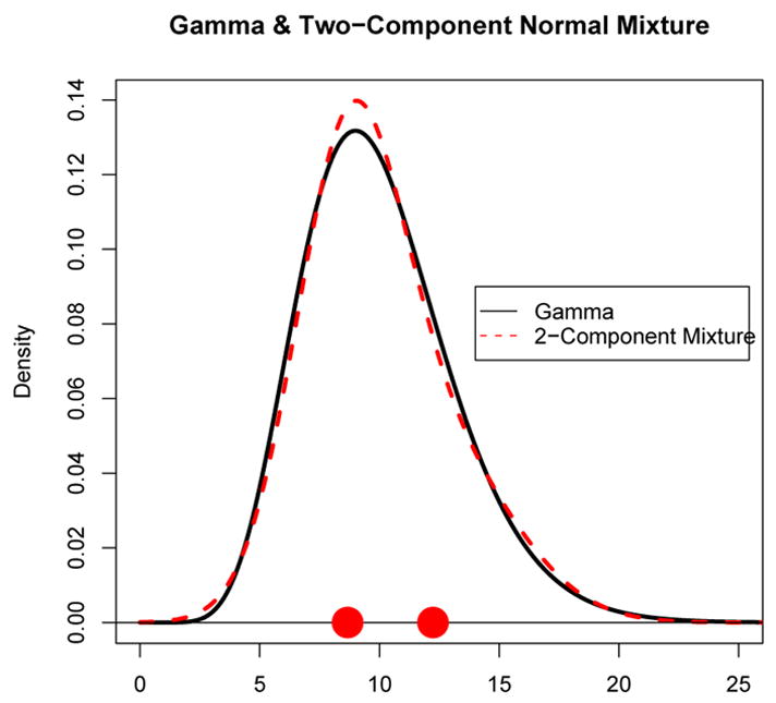
A gamma density (solid curve) with parameters θ = 1, κ = 10 and a two-component normal mixture density (dashed curve) obtained by running the EM algorithm on the gamma distribution. The two points on the x-axis represent the normal mixture component means.

Figure 4 shows the similarities (3.1) between gamma densities and the k = 2 and 3 component normal mixtures obtained from the population-based EM algorithm for shape parameters values ranging from κ = 1 to 20 in increments of 0.25. For small values of κ near 1, there is some discrepancy between the k = 2 and 3 component normal mixture and the gamma distributions, but that discrepancy disappears as κ increases and eventually the gamma distribution and the normal mixtures are indistinguishable. The k = 3 component normal mixture has a higher similarity with the gamma distributions than the k = 2 component mixture as expected. Plotting the ratio of the misspecified population-based log-likelihood (2.8) to the true population-based log-likelihood produces a figure very similar to Figure 4.

Figure 4.

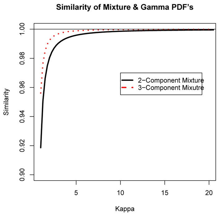
The similarity between gamma densities with shape parameters κ and 2 and 3 component normal mixtures.

3.4 The Skew Normal Distribution

A useful model for skewed distributions is the skew normal distribution (e.g. Azzalini and Capitanio, 1999). In this section we apply the population-based EM algorithm to the skew normal density. The density for a p-dimensional skew normal distribution is

$$2\phi (\mathit{z};\mathbf{\Omega })\mathrm{\Phi }({\mathit{\alpha }}^{\prime }\mathit{z}),$$

where φ is a multivariate normal density with mean zero and correlation matrix Ω, Φ is a univariate standard normal distribution function, and α is a p-dimensional “shape” parameter that controls the degree and direction of skewness. When α = 0, the skew normal density becomes simply a normal density.

Figure 5 shows a one-dimensional skew normal density with shape parameter α = 2 (solid curves). Overlayed is a 2-component mixture in the left panel and a 3-component mixture in the right panel each found using the population-based EM algorithm. The points on the x-axis in left and right panels are the mixture component means. In the left panel of Figure 5, there is very little discrepancy between the skew normal and the 2-component mixture and in the right panel, the density of the skew normal is essentially indistinguishable from the 3-component mixture.

Figure 5.

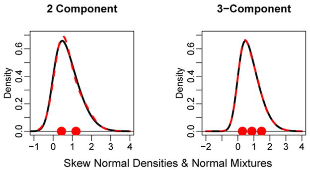
Skew normal densities (solid curves) with shape parameter α = 3. Left Panel: k = 2 component normal mixture and Right Panel: k = 3 component normal mixture (dashed curves). The points are the mixture component means.

Figure 6 shows the similarity between 2 and 3-component mixtures with the univariate skew normal distribution for values of the shape parameter varying from α = 1 to 5. The values of the similarities are very high (ranging from 0.995 to essentially 1). The similarity between the skew normal and the mixtures deteriorates as the shape parameter increases. For instance, eventually, the best fitting 3-component mixture exhibits distinct modes even though the skew normal remains unimodal.

Figure 6.

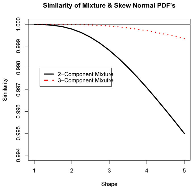
The similarity between skew normal densities with shape parameters ranging from 1 to 5 with k = 2 and 3 component normal mixtures.

The population-based EM algorithm was also applied to the bivariate skew normal distribution. This required numerical evaluation of double integrals which slowed down the EM algorithm substantially and lead to greater numerical error in evaluating the integrals.

Figure 7 shows contours of equal density for a bivariate skew normal distribution with shape vector α = (2, 0)′ and identity correlation matrix, drawn using the skew normal package “sn” package in R (Azzalini, 2006). The population-based EM algorithm was run for k = 4 components and Figure 7 shows two distinctly different solutions in the left and right panels. Reflecting the 4-point pattern in the left panel about the x-axis will produce another 4-component solution as well. Two-dimensional plots of cross-sections of the bivariate skew normal density and the k = 4 component normal mixtures (not shown) show that the conditional mixture densities and the skew-normal densities at these cross-sections are almost identical. Thus, not only can the bivariate skew normal distribution be approximated by a k = 4 component normal mixture, but there exist at least three distinct solutions. In order to compare the two solutions illustrated in Figure 7, the misspecified log-likelihood (2.8) was computed for each solution and surprisingly, the log-likelihoods come out almost identical: −2.465 for the four point pattern in the left panel of Figure 7 and −2.474 for the line pattern in the right panel. Thus, the solution in the left panel leads to a slightly larger misspecified log-likelihood than the line pattern in the right panel. In order to check that the likelihood surface does not form a ridge between these two solutions in the parameter space, the misspecified log-likelihood was evaluated on a set of 10 equally spaced points on the line connecting the two solutions and the misspecified log-likelihood dips in value between these two local maximal solutions. Therefore, the log-likelihood surface does not form a ridge between these two solutions.

Figure 7.

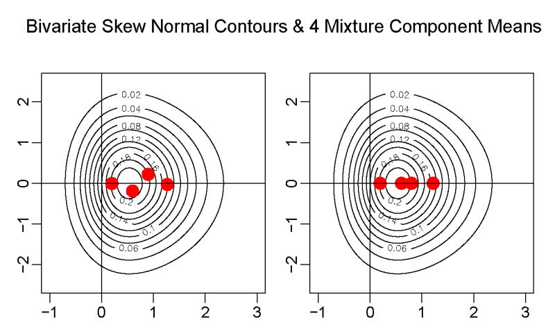
Contours of equal density for a bivariate skew normal with two different solutions for a k = 4 component normal mixture means plotted obtained from the population-based EM algorithm.

The fact that the EM algorithm for a finite mixture can converge to different solutions for the bivariate skew normal distributions mirrors the same phenomenon that occurs with clustering. For instance, for the bivariate normal distribution, there exist many distinct sets of k self-consistent points which are theoretical cluster means for distributions (e.g. see Tarpey, 1998).

Finally, we note that a true mixture model with k components can be misspecified by another mixture model with a different number of components. In fact, determining the number of mixture components is one of the toughest problems in finite mixture modelling. To highlight the problem, Figure 8 shows a k = 3 component normal mixture density (solid curve) and a k = 2 component mixture was fit to this density using the population-based EM algorithm which yielded the dashed density curve in Figure 8. As one can see, there is very little distinction between the k = 2 and k = 3 component mixture densities. The k = 3 mixture component means are plotted with an “x” symbol and the k = 2 component means are plotted with the solid circle on the x-axis.

Figure 8.

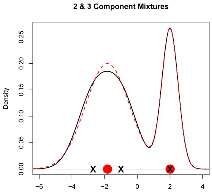
Solid curve is a k = 3 component mixture and the dashed curve is a k = 2 component mixture obtained from the population-based EM algorithm.

This section has illustrated that the EM algorithm for a mixture model will often converge with no problems even if the true distribution is not a mixture (or not a correctly specified mixture in terms of the number of components). Thus, in practice, just because the EM algorithm converges and fits the sample data well, this is not necessarily evidence that the data is from a mixture.

4 Nonparametric Density Estimation Via the Misspecified EM Algorithm

In the previous sections, the EM algorithm for normal mixtures was applied directly to a given density instead of being applied to a data set. Given a set of data, one can estimate a nonparametric density function and then apply the population-based EM algorithm directly to the nonparametric density estimate. Recall that a kernel density estimate is the form

$${\widehat{f}}_h(x)=\frac{1}{nh}\sum _{i=1}^{n}K\left(\frac{x-x_i}{h}\right),$$

where K is a kernel function (e.g. a normal density). Thus, a kernel density estimate is actually an example of a mixture where a mixture component is placed at each data point.

Scott and Szewczyk (2001) propose a procedure for fitting a mixture model by starting with a nonparametric density estimate and then collapsing component densities that are most similar in terms of the similarity index (3.1). Using the population-based EM algorithm, one can proceed in the opposite direction. That is, fit a non-parametric density to the data and then fit a k = 2 component normal mixture using the population-based EM algorithm applied directly to the nonparametric density function. Then, increase the number of components until the similarity between the nonparametric density estimate and the estimated mixture density reaches a specified threshold.

Figure 9 shows the same HAM-D difference histogram as in Figure 1. The solid curve is a nonparametric density estimate. The misspecified population-based EM algorithm for k = 2 components was applied to the nonparametric density and the resulting two component density curve is also plotted (dotted curve). Finally, a two component normal mixture was fit to the raw data using the EM algorithm which produces the dashed density curve in Figure 9. The figure shows that the results of the misspecified population-based EM algorithm coincides very closely to the nonparametric density estimate. However, the fitted mixture from the raw data deviates more substantially from the nonparametric density fit.

Figure 9.

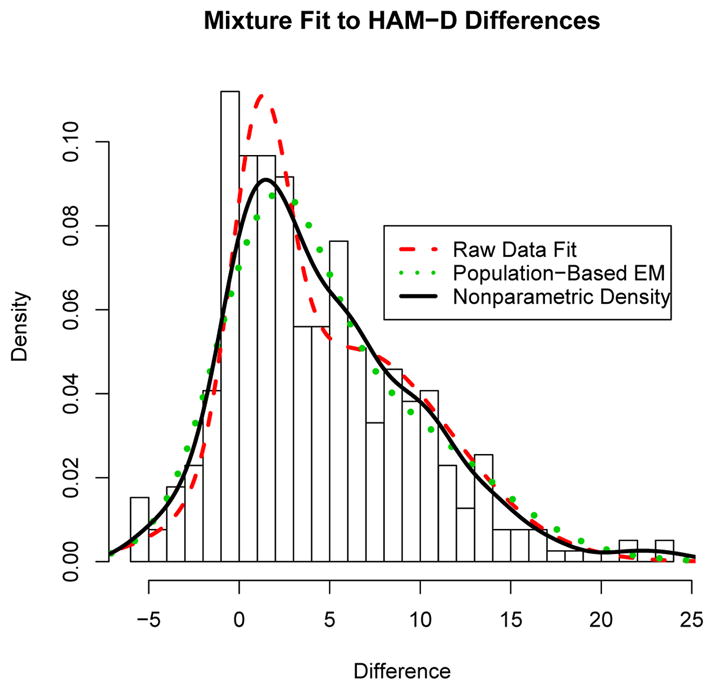
Histogram of the HAM-D difference data with a nonparametric density estimate (solid curve)

5 Clusters or Mixtures?

Consider the problem of defining an illness (e.g. hypertension or depression) in terms of measured variables. Diagnoses are often defined by dividing lines for the variables between illness and no-illness (or different grades of illness). Murphy (1964) states that “There is a fashion which cannot be too strongly condemned of lopping off the end of a distribution curve, endowing it with some pretentious name beginning with ‘hyper-’ and ending with ‘-emia’ or ‘-osis’ and then devoting much effort to seeking the ‘cause’ of it. Well, it is surely a truism that every continuous distribution must have an upper 5 per cent, and by pursuing this idea, as soon as we have defined any measurement we can invent a corresponding disease (page 321).” If the population does indeed consist of distinct groups (e.g. tumor versus no tumor) then “seeking the cause of it” seems reasonable and a mixture model is appropriate. However, in many cases, distinct mixture components may not exist and illness severity will vary along a continuum with respect to measured variables with no clear groupings. Often one can distinguish between individuals at opposite extremes of the continuum. Analogously, a teacher can easily distinguish between an A student and an F student, but the difference between a low A and a high B grade can often be difficult. Nonetheless, a dividing line is needed to assign grades. In medical applications, dividing lines are also often needed in order to make a diagnosis and decide upon a threshold at which a treatment is recommended.

A k-means clustering approach is well-suited for determining dividing lines since the algorithm chops up the distribution into non-overlapping groups. A mixture model on the other hand allows for different groups to overlap provided there exist real distinct groups. If distinct groups do not exist, then cluster means for theoretical homogeneous distributions will nonetheless exist. Flury (1990, 1993) coined the term principal points for cluster means of a theoretical distribution: the points ξ₁, …, ξ_k are k principal points of a random vector Y if

$$E[\underset{j}{min}\parallel \mathit{Y}-{\mathit{\xi }}_j{\parallel }^2]\le E[\underset{j}{min}\parallel \mathit{Y}-{\mathit{y}}_j{\parallel }^2],$$

where y₁, …, y_k is any collection of k points. Tarpey et al. 2003 apply a principal point solution to functional data (quadratic curves) to determine unique response profiles for responders, non-responders, placebo responders, and a mixture of drug/placebo responders in an antidepressant study.

The k-means algorithm provides nonparametric estimators for the k principal points of a distribution. A population-based version of the k-means algorithm can be easily implemented for one-dimensional distributions using the following algorithm: Let Y be a random variable with density function f(y).

Population-Based k-Means Algorithm

1. Begin with initial cluster mean values y₁, …, y_k.

2. Determine cut-points m_j = (y_j + y_j+1)/2, for j = 1, …, k − 1. Set m₀ = −∞ and m_k = ∞.

3. Update the cluster means by computing the conditional expectation of Y between successive cut-points:

$$y_j=\frac{{\int }_{m_{j-1}}^{m_j}yf(y)dy}{{\int }_{m_{j-1}}^{m_j}f(y)dy}.$$

1. Iterate between steps (1) and (2) until successive changes in cluster means are under some threshold.

This procedure will determine the k principal points of a univariate distribution with a precision depending on the accuracy of the numerical integration used to update the cluster means. We implemented the population k-means algorithm for k = 2 in several of the examples in Section 3 and the algorithm usually converged very quickly, much more so than the population-based EM algorithm. In addition, the k = 2 principal points found from the population-based k-means algorithm were often quite close in value to the mixture component means found from the population-based EM algorithm.

The regions of integration formed by the cluster means in 1-dimension are simply intervals (m_j, m_j+1). It would be very difficult to implement the population-based k-means algorithm in higher dimensions because the convex regions needed for the integration formed by the cluster means can take complicated shapes. In higher dimensions there can exist multiple solutions (Tarpey, 1998) for the population-based k-means algorithm, known as self-consistent points (Flury, 1993). Similarly, Figure 7 demonstrates the existence of multiple mixture model solutions for a two dimensional distribution using the population-based EM algorithm. In 1-dimension, there will often be a unique set of k self-consistent points (Trushkin, 1982; Li and Flury, 1995; Tarpey, 1994; Mease and Nair, 2006), for instance if the density is log-concave. It would be interesting to determine if conditions exist that guarantee the existence of a unique set of (non-degenerate) solutions for the population-based EM algorithm.

If the distribution is homogeneous (or even normal), the principal points are well-defined and the k-means algorithm can be used to estimate the principal points of the distribution. However, for homogeneous distributions, the mixture component means found from fitting a finite mixture model are (no pun intended) meaningless.

On the other hand, if the distribution is really a finite mixture, then the EM algorithm produces approximately unbiased estimates via maximum likelihood of the mixture model parameters. The k-means algorithm will still converge to consistent estimators of principal points but the principal points and the mixture component means do not coincide. For instance, for a univariate k = 2 normal mixture with component means μ±δ, equal prior probabilities and variance σ² in each component, the two principal points will be equal to

$$\mu \pm [2\delta \mathrm{\Phi }(\delta /\sigma )-\delta +\sqrt{\frac{2}{\pi }}\sigma e^{-{\delta }^2/(2{\sigma }^2)}],$$

which differs from the true mixture component means. Hartigan (1978) proposes a test of normality versus a k = 2 component normal mixture based on the fact that the cluster means from the k-means algorithm are biased for the true mixture component means. Note that as the mixture component means move apart (i.e. as δ increases), the k = 2 principal points converge to the true mixture component means.

6 Discussion

It is well known that any given continuous distribution can be approximated by a mixture model. We have demonstrated through the population-based EM algorithm that mixture models with as few as two or three mixture components can provide a very good approximation to some well-known non-normal homogeneous distributions. We have not attempted the reverse, i.e., to determine if there exists a parametric family of non-normal homogeneous distributions that can approximate arbitrarily well a given mixture density.

Everitt (1981) writes, “…it may be more appropriate for workers in this area (depression) to consider fitting mixtures to their data in their attempts to gain evidence for or against the existence of two types of depression (page 338).” Unfortunately, determining that a mixture distribution provides a better fit to the data than a normal (i.e. k = 1 component mixture) distribution is not evidence that the underlying distribution is a mixture, for, as we have shown, the underlying distribution could be some other non-normal, but homogeneous distribution. Bimodality in large samples is often (but not always, see Tarpey and Petkova (2007)) evidence of at least two distinct sub-populations. Of course, this will only occur if the mixture component means are well separated and/or the mixture component variances are relatively small. Powerful statistical techniques are essential in cases when the mixtures are not well-separated, but unfortunately, in these cases, we will not always be able to distinguish a mixture from some other homogeneous non-normal distribution. The problem is compounded because the mixture model and the homogenous non-normal probability model present two very different models for reality.

Several authors have pointed out the danger of assuming the existence of a mixture. For instance, Marriott (1971) states that “it is unsafe to assume that departure from a known distributional form is an indication of a compound distribution (page 506).” Dunn et al. 1993 point out in discussing statistics and the nature of depression that “Bimodality provides strongly suggestive evidence that there are two groups, but the lack of it does not imply the opposite (page 72).” When bimodality is not present, Pearson (1895) expressed optimism that a method would eventually be found to distinguish consistently between a mixture and a skew curve (page 395). However, as shown in this paper, there exist homogeneous non-normal densities that are essentially the same as k = 2 and 3 component mixtures which dashes the optimism expressed by Pearson.

References

- Azzalini A. R package sn:The skew-normal and skew-t distributions (version 0.4-0) Universit di Padova; Italia: 2006. [Google Scholar]
- Azzalini A, Capitanio A. Statistical applications of the multivariate skew-normal distribution. Journal of the Royal Statistical Society, series B. 1999;61:579–602. [Google Scholar]
- Bauer DJ, Curran PJ. Distributional assumptions of growth mixture models: Implications for overextraction of latent trajectory classes. Psychological Methods. 2003;8:338–363. doi: 10.1037/1082-989X.8.3.338. [DOI] [PubMed] [Google Scholar]
- Dempster AP, Laird NM, Rubin DB. Maximum likelihood from incomplete data via the EM algorithm. Journal of the American Statistical Association. 1977;39:1–38. [Google Scholar]
- Dunn G, Sham PC, Hand DJ. Statistics and the nature of depression. Journal of the Royal Statistical Society, Series A. 1993;156:63–87. [Google Scholar]
- Everitt BS. Bimodality and the nature of depression. British Journal of Psychiatry. 1981;138:336–339. doi: 10.1192/bjp.138.4.336. [DOI] [PubMed] [Google Scholar]
- Fang KT, Wang Y. Number-Theoretic Method in Statistics. Chapman and Hall; London: 1994. [Google Scholar]
- Flury B. Principal points. Biometrika. 1990;77:33–41. [Google Scholar]
- Flury B. Estimation of principal points. Applied Statistics. 1993;42:139–151. [Google Scholar]
- Forgy EW. Cluster analysis of multivariate data: efficiency vs interpretability of classifications. Biometrics. 1965;21:768–769. [Google Scholar]
- Hartigan JA. Asymptotic distributions for clustering criteria. Annals of Statistics. 1978;6:117–131. [Google Scholar]
- Hartigan JA, Wong MA. A k-means clustering algorithm. Applied Statistics. 1979;28:100–108. [Google Scholar]
- Li L, Flury B. Uniqueness of principal points for univariate distributions. Statistics and Probability Letters. 1995;25:323–327. [Google Scholar]
- MacQueen J. Some methods for classification and analysis of multivariate observations. Proceedings 5th Berkeley Symposium on Mathematics, Statistics and Probability. 1967;3:281–297. [Google Scholar]
- Marriott Practical problems in a method of cluster analysis. Biometrics. 1971;27:501–514. [PubMed] [Google Scholar]
- McLachlan GJ, Krishnan T. The EM Algorithm and Extensions. Wiley; New York: 1997. [Google Scholar]
- Mease D, Nair VN. Unique optimal partitions of distributions and connections to hazard rates and stochastic ordering. Statistica Sinica. 2006 To appear. [Google Scholar]
- Murphy EA. One cause? many causes? the argument from the bimodal distribution. Journal of Chronic Diseases. 1964;17:301–324. doi: 10.1016/0021-9681(64)90073-6. [DOI] [PubMed] [Google Scholar]
- Pearson K. Contributions to the mathematical theory of evolution. ii. skew variation in homogeneous material. Philisophical Transactions of the Royal Society of London. 1895;186:343–414. [Google Scholar]
- Piessens R, de Doncker-Kapenga E, Uberhuber C, Kahaner D. QUADPACK, A Quadrature Subroutine Package, Series in Computational Mathematics. Springer-Verlag; Berlin: 1983. [Google Scholar]
- R Development Core Team. R: A language and environment for statistical computing. R Foundation for Statistical Computing; Vienna, Austria: 2003. [Google Scholar]
- Scott DW, Szewczyk WF. From kernels to mixtures. Technometrics. 2001;43:323–335. [Google Scholar]
- Swartz T, Evans M. Approximating Integrals Via Monte Carlo and Deterministic Methods. Oxford University Press; 2000. [Google Scholar]
- Tarpey T. Two principal points of symmetric, strongly unimodal distributions. Statistics and Probability Letters. 1994;20:253–257. [Google Scholar]
- Tarpey T. Self-consistent patterns for symmetric multivariate distributions. Journal of Classification. 1998;15:57–79. [Google Scholar]
- Tarpey T, Petkova E. Latent regression analysis Submitted for publication. 2007 doi: 10.1177/1471082X0801000202. [DOI] [PMC free article] [PubMed] [Google Scholar]
- Tarpey T, Petkova E, Ogden RT. Profiling placebo responders by self-consistent partitions of functional data. Journal of the American Statistical Association. 2003;98:850–858. [Google Scholar]
- Titterington DM, Smith AFM, Makov UE. Statistical Analysis of Finite Mixture Distributions. Wiley; New York: 1985. [Google Scholar]
- Topsøe F. Basic concepts, identities and inequalities – the toolkit of information theory. Entropy. 2001;3:162–190. [Google Scholar]
- Trushkin A. Sufficient conditions for uniqueness of a locally optimal quantizer. IEEE Transactions in Information Theory. 1982;28:187–198. [Google Scholar]