Estimating large-scale signaling networks through nested effect models with intervention effects from microarray data

Abstract

Motivation: Targeted interventions using RNA interference in combination with the measurement of secondary effects with DNA microarrays can be used to computationally reverse engineer features of upstream non-transcriptional signaling cascades based on the nested structure of effects.

Results: We extend previous work by Markowetz et al., who proposed a statistical framework to score different network hypotheses. Our extensions go in several directions: we show how prior assumptions on the network structure can be incorporated into the scoring scheme by defining appropriate prior distributions on the network structure as well as on hyperparameters. An approach called module networks is introduced to scale up the original approach, which is limited to around 5 genes, to infer large-scale networks of more than 30 genes. Instead of the data discretization step needed in the original framework, we propose the usage of a beta-uniform mixture distribution on the P-value profile, resulting from differential gene expression calculation, to quantify effects. Extensive simulations on artificial data and application of our module network approach to infer the signaling network between 13 genes in the ER-α pathway in human MCF-7 breast cancer cells show that our approach gives sensible results. Using a bootstrapping and a jackknife approach, this reconstruction is found to be statistically stable.

Availability: The proposed method is available within the Bioconductor R-package nem.

Contact: h.froehlich@dkfz-heidelberg.de

1 INTRODUCTION

The advent of RNA silencing enables researchers to selectively silence genes of interest on large scale. DNA microarrays allow to measure the effects of a perturbation on a genome-wide scale. This enables to reverse engineer interdependencies between gene products on a non-transcriptional level. The genes of interest are silenced individually, and the respective downstream effects on gene expression are measured by using genome-wide microarrays. By observing the nested structure of significant up- or down-regulations of affected genes, this allows to reconstruct features of the upstream signaling pathway (Boutros et al., 2002).

In a recent work, Markowetz et al. (2005) introduced nested effect models as a method to reverse engineer the signal flow between perturbed genes using the nested subset relationship of secondary downstream effects. They developed a Bayesian statistical framework, in which for a given network hypothesis one can calculate a score and thus can reduce the set of all possible networks to the most likely ones. A severe limitation of this method lies, however, in the restriction to small networks of up to five genes, because the method completely enumerates all possible network hypotheses. Furthermore, a difficulty in the practical use is the required binary discretization of the data (‘secondary effect present/not present’).

In our work, we extend the framework by Markowetz et al. in several directions in order to overcome these restrictions: instead of the data discretization step needed in the original framework, we propose the usage of a beta-uniform mixture distribution on the P-value profile, resulting from differential gene expression calculation, to quantify effects (Pounds and Morris, 2003). Moreover, we show how prior assumptions on the network structure can be incorporated into the network scoring scheme by defining appropriate prior distributions on the network structure as well as on its hyperparameter. Finally, and most important, we present our so-called module networks to scale up the original approach, which is limited to small pathways with around five genes, to the inference of large-scale networks (up to more than 30 genes). The idea is to build the complete network recursively from smaller pieces that are connected subsequently. In order to validate our approach, we conduct extensive simulations on artificially created networks and compare it to the triplets inference scheme described in Markowetz et al. (2007). We show that module networks offer a better performance in terms of reconstruction quality while being significant computationally faster at the same time. We also apply our module networks to infer the signaling network between 13 genes in the ER-α pathway in human MCF-7 breast cancer cells. Using bootstrapping and the jackknife this reconstruction is found to be statistically stable.

2 METHODS

2.1 Original approach

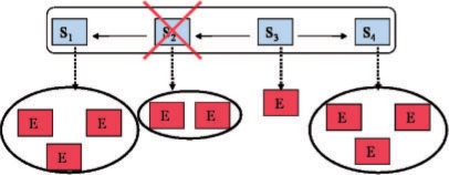
We start with a brief review of the framework by Markowetz et al.: in general one distinguishes between silenced genes (S-genes) and genes showing a downstream effect (E-genes). It is assumed that each E-gene is attached to a single S-gene only (Fig. 1). Knocking down a specific S-gene S_k interrupts signal flow in the downstream pathway, and hence an effect on the E-genes attached to S_k and all S-genes depending on S_k is expected. Let us assume n knock-downs are performed and there exist m E-genes in total. The outcomes of these experiments are summarized in an m × n data matrix D. According to Bayes' formula, a specific network hypothesis Φ ∈ {0, 1}ⁿ × {0, 1}ⁿ can be scored as:

(1)

The position of the E-genes is introduced as a model parameter Θ = {θ_i|θ_i∈ {1, …, n}, i = 1, …,m}, i.e. θ_i = j, if E-gene i is attached to S-gene j. Assuming independence of the observations (rows) D_i in the data matrix D (given a fixed network hypothesis Φ and model parameters Θ) one can write down the conditional likelihood P(D|Φ, Θ) as:

(2)

It is furthermore assumed that all parameters θ_i are statistically independent, i.e.

(3)

The likelihood P(D|Φ) can then be written as:

(4)

(5)

We now suppose a decomposition of P(D_i|Φ,θ_i) as follows:

(6)

This makes the assumption that knock-down experiments are statistically independent from each other. Hence, Equation (5) can be written down as

(7)

Fig. 1.

Main idea of the inference framework by Markowetz et al.: a network hypothesis is a directed graph between S-genes. Attached to each S-gene are several E-genes. Knocking down S-gene S₂ interrupts signal flow in the downstream pathway, and hence an effect of E-genes attached to S₂ and to S₁ is expected.

2.2 Extensions

2.2.1 Generalized inference framework

Markowetz et al. suppose the data matrix D to consist of counts, how often a specific E-gene shows an effect in ℓ experiment repetitions. This requires a data discretization step, for which user-specified type-I and type-II error rates are assumed. The choice of these parameters is critical for the inference procedure, because it directly influences (6) and is difficult to estimate. Markowetz et al. suppose to have both, positive and negative controls (pathway stimulated/not stimulated) for this procedure, which for our data is not available (Section 3.2).

In our approach we only make the quite general assumption that D is an m × n matrix of (raw) P-values, which specify the likelihood of E-gene i being differentially expressed after knock-down of S-gene k. The P-values are calculated using an arbitrary method for detecting differential gene expression, e.g. limma (Smyth, 2004). They are supposed to be drawn from a mixture of a uniform [0, 1] distribution reflecting the null hypothesis and another distribution f₁ reflecting the alternative hypothesis (Pounds and Morris, 2003):

(8)

Under the alternative hypothesis, there is a high density for small P-values and a strong decrease for increasing P-values. Both distributions overlap with mixing coefficient γ_k · P (D_ik|Φ,θ_i) can therefore be decomposed as:

(9)

The density function f₁ reflects the strength of the knock-down effect on E-gene i under the alternative hypothesis. If it is greater than 1 the alternative hypothesis would be accepted, and if it is smaller than 1 rejected. Still the problem remains, how to define f₁ appropriately. For this purpose one may simply assume a single Beta (1, β_k) (β_k > 2) distribution (c.f. Fröhlich et al., 2007a, b). However, a better fit can be obtained by modeling P(D_ik) : = f(D_ik) as a three component mixture of a uniform, a Beta(1, β_k) (β_k > 2) and a Beta (α_k, 1) (α_k < 1) distribution:

(10)

with π_1k + π_2k + π_3k = 1 (π_rk ≥ 0, r = 1, 2, 3). This three component beta-uniform mixture model (BUM) can be fitted via an EM algorithm (Dempster et al., 1977). The alternative distribution f₁ can then be extracted as follows: Let be the maximum uniform part of the BUM model. Then

(11)

Figure 2 shows an example histogram of a P-value distribution resulting from one of our real-life experiments, which are explained in detail in Section 3.2. As seen the model curve drawn in black fits the histogram perfectly. The extracted alternative distribution is shown in red.

Fig. 2.

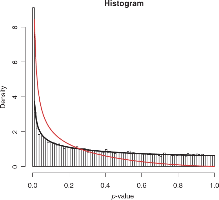
Histogram of the P-value distribution of AKT2 knock-down (see Section 3.2). Black: mixture model curve; red: extracted alternative distribution.

2.2.2 A Bayesian prior on the network structure

Equation (1) allows to specify a prior P(Φ) on the network structure itself. This can be thought of biasing the score of possible network hypotheses towards prior knowledge or assumptions. At the same time, we have to take into account that our assumptions may only be true up to a certain degree. Hence, for each edge we should suppose a prior probability reflecting the degree of belief in its existence. In principle, this degree of belief can be very different for each edge. We summarize all prior edge probabilities in an n × n matrix . Making the assumption that all edge priors P(Φ_ij) are independent, i.e.

(12)

allows us to define the connection between Φ_ij and for each edge separately. Note that Φ_ij ∈ {0, 1} depending on whether we set the edge i → j or not. Hence, for each edge we have a certain difference to our prior assumptions. The smaller this difference, the higher P(Φ_ij) should be. We can therefore model P(Φ_ij) as a Laplacian distribution with width parameter ν (cf. Imoto et al., 2003):

(13)

The width parameter ν can scale the prior in an adjustable way. From a Bayesian perspective one should hence specify a prior on the parameter ν as well. A natural choice for this purpose is the inverse gamma distribution with hyperparameters 1 and 0.5:

(14)

The full edge prior P(Φ_ij) can then be obtained via marginalization:

(15)

If the difference to our prior assumptions is zero, then the prior is 1, whereas for the prior superlinearly drops to 1/9.

2.2.3 Large-scale network inference

The inference framework (Sections 2.1 and 2.2.1), does not answer the question how to come up with a candidate network topology, which we would like to score. Markowetz et al. (2005) completely enumerate all possible topologies. This is, however, only suitable for small networks of up to 5 S-genes. For 5 S-genes there already exist more than 1 000 000 and for 10 genes more than 10²⁷ possible network topologies. In this context it should be noted that the scoring scheme (Section 2.1) cannot distinguish between two network hypotheses, if they only differ in transitive edges. This issue is known as prediction equivalence and is due to the fact that subset relationships, which are represented by a nested effects model, are transitive in principle. Hence, it only makes sense to consider the set of all transitively closed network hypotheses. However, restricting ourselves to this limited class of network structures does not generally solve the problem, since even then the number of networks to consider scales in a similar way with the number of S-genes. Hence, we have to resort to heuristics.

Module networks: The idea of the module network is to build up a graph from smaller subgraphs, called modules in the following. Here we present an updated version of the algorithm presented in our earlier publications (Fröhlich et al., 2007a, b).

We begin with a hierarchical clustering of the preprocessed expression profiles of all S-genes, e.g. via average linkage. The idea is that S-genes with a similar E-gene response profile (here: with regard to the Pearson correlation similarity) should be close in the signaling path. We now successively move down the cluster tree hierarchy until we find a cluster with only 4 S-genes at most. Figure 3 illustrates the idea with an assumed network of 10 S-genes. At the beginning we find S₈ as a cluster singleton. Then by successively moving down the hierarchy we identify clusters S₆, S₇, S₁, S₁₀, S₃, S₂, S₅ and S₄, S₉. All these clusters (modules) contain 4 S-genes at most and can thus be estimated by taking the highest scoring of all possible network hypotheses.

Fig. 3.

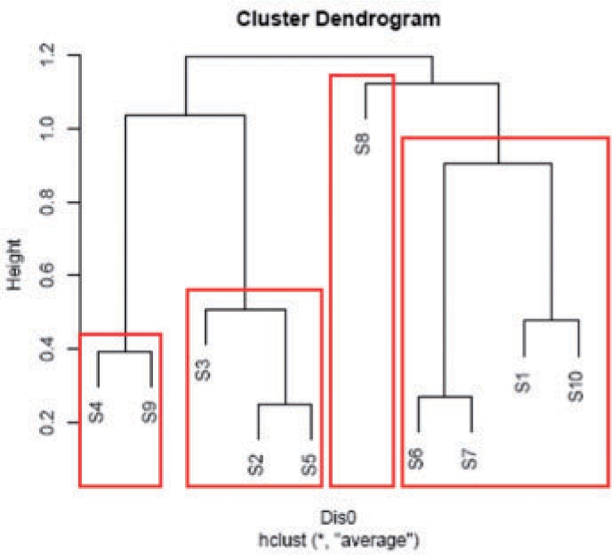
Basic idea of module networks: by successively moving down the cluster hierarchy we identify the clusters (modules) of S-genes, which are marked in red. They contain 4 S-genes at most and can be estimated by exhaustively searching for the highest scoring model.

Once all modules have been estimated their connections are constructed. This is done in a constraint greedy hill-climbing fashion: we successively add that edge between any pair of S-genes being contained in different modules, which increases the likelihood of the complete network most. This procedure is continued until no improvement can be gained any more, i.e. we have reached a local maximum of the likelihood function.

3 EXPERIMENTS

3.1 Large-scale inference: evaluation on artificial networks

To test our methods and to get better insights into the performance of our large-scale inference methods, we generated data from artificial random networks.

3.1.1 Network topology creation

Artificial random networks were generated as follows: For each node S_k we randomly chose the number o of outgoing edges between 0 and 3. We then selected o nodes having at most 1 ingoing edge, connected S_k to them and transitively closed the graph. Averaged over 100 random networks for n = 10, this procedure yielded an average of 3.5 ± 2.1 ingoing and 3.5 ± 3.6 outgoing edges per node (min. 0, max. 9 in both cases). After network topology construction, the m E-genes were attached uniform randomly over all S-genes.

3.1.2 Data sampling

We then simulated knock-downs of the individual S-genes. For those E-genes, where no effects were expected, the ‘P-values’ were drawn uniform randomly from [0, 1]. For the others there was an independent prior effect probability depending on the path distance d to the ‘knocked-down’ S-gene of , i.e. at the maximal achievable path distance of d = n − 1 there was only a 50% chance to observe an effect. For each E-gene we threw a biased coin with the corresponding prior effect probability, and depending on the outcome the ‘P-value’ was either again drawn uniform randomly from [0, 1] or sampled from the alternative distribution [Equation (8)]. In order to do so we sampled random parameters α_k ∈ (0, 1), β_k ∈ [5, 50] and π_2k, π_3k ∈ (0, 0.5) (note that π_1k = 1 − π_2k − π_3k) of the three component BUM model [Equation (10)] for each ‘knocked-down’ separately. That means for each S-gene the ‘P-values’ could have a different distribution. To take into account the BUM model re-estimation error, we additionally blurred each parameter with normally distributed noise (SD β_k: 10%; other parameters: 0.05). These ‘noisy’ parameters were then used to draw ‘P-values’ from the alternative distribution. However, to quantify the effect strength according to Equation (11) the original parameters were used. Hence, we simulated a mismatch between the empirical and the modeled ‘P-value’ distribution.

3.1.3 Simulation results

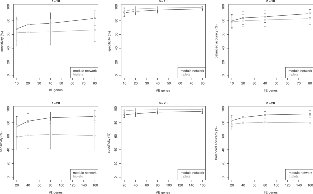
We sampled networks with n = 10, 20, 30 S-genes. For each number of S-genes we varied the number m = n, 2n, 4n, 8n of E-genes. We compared the module network with the triplets inference approach described in Markowetz et al. (2007). The idea of the latter is to decompose the complete network in all possible combinations of three S-genes. For each triplet the highest scoring model can then be found among all 29 possible ones. No prior knowledge on the network structure was used. We evaluated both methods in terms of average sensitivity (i.e. ratio of correctly learned edges to total number of edges in the original network) and specificity (i.e. ratio of correctly unconnected genes to total number of unconnected genes in the original network over 10n generated networks for n S-genes. Moreover, the balanced accuracy, i.e. the average of sensitivity and specificity was computed.

In Figure 4, we show the results for n = 10, 20 S-genes. While module networks and the triplets inference algorithm yield a comparable specificity, the sensitivity for module networks is much higher. As a result, the balanced accuracy for module networks differs from that of the triplets inference algorithm significantly for all numbers of E-genes. This conclusion was assessed by a pairwise t-test at significance level 0.05. At the same time, the computation time for the triplets inference was significantly higher (Fig. 5) than for the module networks. For n = 30 S-genes triplets inference already became impractically slow, so that we omit results here. In contrast, the module network only needed around 2 min for one network inference on average, which seems affordable. As indicated by the plots in Figure 6, the network reconstruction quality does not differ much from that for n = 10, 20.

Fig. 4.

Simulation results for artificial networks with n = 10, 20 S-genes and varying number of E-genes.

Fig. 5.

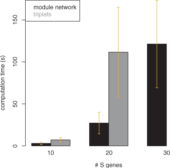
Computation times (s) for module networks and triplets inference. For n = 30 triplets inference already becomes impractically slow.

Fig. 6.

Simulation results for artificial networks with n = 30 S-genes and varying number of E-genes (module networks).

Next we investigated the effect of the network prior [Equation (15)]. For each network we randomly picked 25%, 50%, 75% of all edges in the original network (true positives) and included 5% false positives. For both, true and false positives, the prior edge probability was set to 100%. Figure 7 summarizes the average improvement in terms of sensitivity, specificity and balanced accuracy, which is gained by our prior for the module network. As expected, the sensitivity is highly increased, especially for a lower number of E-genes. At the same time the specificity for m > 10 remains almost constant. In conclusion, for all numbers of E-genes a significant improvement of the balanced accuracy can be gained (P < 0.05).

Fig. 7.

Average improvement by prior knowledge of 25%, 50%, 75% true posititive and 5% false-positive edges with varying number of E-genes (n = 10 S-genes, module networks).

3.2 Application to RNAi data from human ER-α pathway

3.2.1 Data

We applied the module network to infer the complete topology for a network of n = 13 S-genes in the ER-α pathway. The 13 genes were selected from previous microarray studies in our department to be influenced by ER status in breast cancer patients. Each of the 13 genes was silenced individually using two different siRNAs, respectively, and the effect on gene expression was studied on whole genome cDNA microarrays. The data were generated in our department. Details are omitted here due to restrictions of space, but can be obtained from the authors.

3.2.2 Preprocessing

For each knock-down experiment after VSN normalization (Huber et al., 2002) P-values for differential gene expression detection were calculated using limma (Smyth, 2004). Afterwards BUM models were fitted to quantify effects as described in Section 2.2.1. An a priori filtering among the joint set of the top 100 E-genes from each experiment was performed to select patterns of differentially expressed genes that can be expected to be non-randomly: supposed a gene is significantly non-differentially expressed in knock-down experiment k. Nonetheless we can observe a (multiple testing corrected) P-value < α with false-positive rate α. Let us encode with 1, if the P-value is smaller than α and 0 otherwise. For n knock-down experiments, we can summarize the outcome for each E-gene in a binary vector b = (b₁, …, b_n)^T. Let M be the total number of E-genes and s_k the number of significant genes in experiment k. Then, under the null hypothesis the probability to observe b just by chance is

(16)

Among M E-genes we can thus expect to see b Pr(b|H₀)M times just be chance. The statistical significance of observing b more often than can be expected by chance can therefore be assessed by a binomial test. The corresponding P-value for each pattern is corrected for multiple testing using the Bonferroni method later. We then only choose those E-genes, which show a significant pattern. In conclusion this procedure eliminates false-positive patterns and thus reduces the noise in the data. Moreover, the dimensionality of the data is reduced efficiently. For our data we arrived at m = 621 E-genes this way.

3.2.3 Network inference

We ran both, the triplets inference algorithm and the module network reconstruction on our dataset. We found the log marginal likelihood of the triplets inference algorithm network to be significantly lower than that of the module network (likelihood difference 142), thus supporting our conclusions drawn from the simulation studies.

For our final network reconstruction we employed bootstrapping in order to ensure the statistical stability and robustness of the solution: we sampled m E-genes from the total set of E-genes 1000 times with replacement and each time ran the module network for topology induction. We did not use any of the literature knowledge for inference here in order to have an external source of validation later on. We only considered edges, which were found in more than 50% of all bootstrap trials. The average bootstrap probability for these edges was 90 ± 14%, i.e. most edges were inferred with high stability. Furthermore, we assessed the stability of the reconstructed network in a different way via jackknifing: Each S-gene was left out once and the network inferred on the present S-genes. We then counted the frequency of each edge among all n network reconstructions. Only edges with a jackknife probability of more than 50% were considered. The average probability of these edges was 86 ± 11%, i.e. again most edges were highly stable. The overlap of the results obtained from bootstrapping and from the jackknife is depicted in Figure 8 as a transitively reduced graph.¹

Fig. 8.

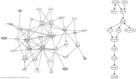
Left: Literature network obtained from Ingenuity™. Right: Consensus network induced by our method (transitively reduced graph).

3.2.4 Comparison with literature

We performed a literature scan for known interdependencies between S-genes using the Ingenuity™ Software (Fig. 8, left). The edge ESR1 → AKT2 in our network reconstruction is reflected by the signaling cascade ESR1 → Hsp70 → AKT1 → TCL1B → AKT2. Likewise, AKT2 → BCL2 → AKT1 can be confirmed by the signaling cascade AKT2 → ESR1 → BCL2 → Hsp90 → AKT1. Furthermore, our network contains BCL2 → STAT5B, which in the literature is BCL2 → PPP2CA → PTPN7 → STAT5B, and STAT5B → ERK2 → FOXA1, which is reflected by STAT5B → PTPN7 → ERK2 → TP53 → Hist3 → FOXA1. At this point it should also be mentioned that due to experimental circumstances in RNAi knock-down experiments and due to the used cell line in principle there might be deviances of the literature knowledge to the measured data.

4 CONCLUSION

We proposed a method for reconstructing signaling pathways from secondary effects, which were observed on microarray after silencing genes of interest via RNAi. Our approach systematically extends and generalizes previous work by Markowetz et al. instead of data discretization, a beta-uniform mixture distribution on the P-value profile resulting from differential gene expression calculation was used, to quantify effects. A Bayesian prior on the network structure was developed to incorporate assumptions on the network structure. In our simulation studies, we could show that in principle this way the sensitivity of network reconstruction can be increased significantly.

We developed an algorithm for large-scale inference of signaling pathways and evaluated in a systematic fashion on artificially created data. Our module networks, which recursively build up the complete topology from smaller pieces, were found to have a significantly better network reconstruction quality than the previously proposed triplets inference algorithm (Markowetz et al., 2007). At the same time, our module networks could be computed much faster and therefore allowed for the inference of large-scale networks of more than 30 genes.

We used the module network to infer the signaling pathway for 13 genes in the ER-α pathway in human MCF-7 breast cancer cells and used a bootstrapping as well as a jackknife approach to ensure the statistical stability of the result. The induced edges in our inferred network were found with high consistency and could partially be also confirmed by the literature. Future biological experiments are planned to validate our reconstructed network in a systematic way. In conclusion of our results we think that our approach offers a scalable, reliable and fairly general way for large-scale inference of signaling pathways from secondary effects and therefore provides researchers with a valuable tool to gain insight into complex cellular processes.

The code for the module network inference method is available in the latest version of the R-package nem, which can be obtained from the Bioconductor homepage.

REFERENCES

- Aho A, et al. The transitive reduction of a directed graph. SIAM J. Comput. 1972;1:131–137. [Google Scholar]
- Boutros M, et al. Sequential activation of signaling pathways during innate immune responses in Drosophila. Dev. Cell. 2002;3:711–722. doi: 10.1016/s1534-5807(02)00325-8. [DOI] [PubMed] [Google Scholar]
- Dempster A, et al. Maximum likelihood from incomplete data via the em algorithm. J. Royal Statistical Soc., Series B. 1977;39:1–38. [Google Scholar]
- Fröhlich H, et al. Estimating large scale signaling networks through nested effects models from intervention effects in microarray data. Proceedings German Conf. on Bioinformatics. 2007a doi: 10.1093/bioinformatics/btm634. Gesellschaft für Informatik, pp. 45–54. [DOI] [PMC free article] [PubMed] [Google Scholar]
- Fröhlich H, et al. Large scale statistical inference of signaling pathways from rnai and microarray data. BMC Bioinformatics. 2007b;8:386. doi: 10.1186/1471-2105-8-386. [DOI] [PMC free article] [PubMed] [Google Scholar]
- Huber W, et al. Variance stabilization applied to microarray data calibration and to the quantification of differential expression. Bioinformatics. 2002;18:S96–S104. doi: 10.1093/bioinformatics/18.suppl_1.s96. [DOI] [PubMed] [Google Scholar]
- Imoto S, et al. Combining microarrays and biological knowledge for estimating gene networks via bayesian networks. Proceedings 2nd Computational Systems Bioinformatics. 2003:104–113. [PubMed] [Google Scholar]
- Markowetz F, et al. Non-transcriptional pathway features reconstructed from secondary effects of rna interference. Bioinformatics. 2005;21:4026–4032. doi: 10.1093/bioinformatics/bti662. [DOI] [PubMed] [Google Scholar]
- Markowetz F, et al. Nested effects models for high-dimensional phenotyping screens. Bioinformatics. 2007;23:i305–i312. doi: 10.1093/bioinformatics/btm178. [DOI] [PubMed] [Google Scholar]
- Pounds S, Morris S. Estimating the occurence of false positives and false negatives in microarray studies by approximating and partitioning the empirical distribution of P-values. Bioinformatics. 2003;19:1236–1242. doi: 10.1093/bioinformatics/btg148. [DOI] [PubMed] [Google Scholar]
- Smyth G. Linear models and empirical bayes methods for assessing differential expression in microarray experiments. Stat. Appl. Genet. Mol. Biol. 2004;3 doi: 10.2202/1544-6115.1027. [DOI] [PubMed] [Google Scholar]