α-Helical Topology Prediction and Generation of Distance Restraints in Membrane Proteins

Abstract

The field of protein structure prediction has seen significant advances in recent years. Researchers have followed a multitude of approaches, including methods based on comparative modeling, fold recognition and threading, and first-principles techniques. It is noteworthy that the structure prediction of membrane proteins is comparatively less studied by researchers in the field. A membrane protein is characterized by a protein structure that extends into or through the lipid-lipid bilayer of a cell. The structure is influenced by the combination of the hydrophobic bilayer region, the direct interaction with the bilayer, and the aqueous external environment. Due to the difficulty in obtaining reliable experimental structures, accurate computational prediction of membrane proteins is of paramount importance. An optimization model has been developed to predict the interhelical interactions in α-helical membrane proteins. A database of α-helical membrane proteins of known structure and limited sequence identity can be constructed to develop interaction probabilities. By then maximizing the occurrence of highly probable pairwise or three-residue interactions, realistic contacts can be predicted by imposing a number of geometrical constraints. The development of these low distance contacts can provide additional distance restraints for first principles-based approaches to the tertiary structure prediction problem. The proposed approach is shown to successfully predict interhelical contacts in several membrane protein systems, including bovine rhodopsin and the recently released human β2 adrenergic receptor protein structure.

INTRODUCTION

Despite the multitude of available methods for protein structure prediction, the advances in the study of membrane proteins have not been as quick to follow. Whereas there are more than 46,000 experimentally determined structures available through the Protein Data Bank (1), only 144 proteins are membrane proteins with experimentally validated transmembrane segments (2). Due to the difficulty in obtaining reliable experimental structures, accurate theoretical prediction of membrane proteins is of paramount importance. This significance becomes even more striking given the number of membrane proteins and their role in drug development. It has been estimated that integral membrane proteins make up ∼20–30% of the total proteins across a variety of organisms (3,4). As much as 30% of commercial drugs are known to target G-protein-coupled receptors (5), a family of membrane proteins characterized by an α-helical bundle of seven helices.

Although it is difficult to crystallize membrane proteins to determine their three-dimensional structure, the analysis of membrane topology through biochemical methods is much more feasible. There have been major advances in the prediction of transmembrane regions of proteins. Due to the distinctive patterns of hydrophobic regions within the membrane and polar loop regions beyond the membrane, hydrophobicity and polarity have been used to predict these regions. These methods can be evaluated based on their ability to correctly predict the membrane-spanning regions, as well as the sidedness of a protein. One popular method, TMHMM, uses a global implementation of a hidden Markov model to make its predictions (3). Different approaches, such as MEMSAT, are based on a combined form that accounts for local level effects and incorporates them into global heuristics (6). Independent studies of these types of prediction methods have identified MEMSAT and TMHMM as high-performing methods in this area, although prediction performance was less impressive for eukaryotic proteins (7,8). Recent contributions in this area have considered combining a hidden Markov model with evolutionary information (9), combining a hidden Markov model with a molecular mechanics energy-scoring function (10), applying a support vector machine algorithm (11), and combining a variety of algorithms through a consensus approach (12).

Since a large percentage of membrane proteins form α-helical bundles, many efforts have been made to compare and contrast these proteins with soluble α-helical proteins. Membrane proteins seem to satisfy the backbone hydrogen bonds in the low dielectric environment (13). Eilers et al. have used the technique of occluded surface to demonstrate that membrane proteins have higher packing values than soluble proteins (14). Part of the reasoning behind this effect is the tendency of membrane proteins to have a higher occurrence of small amino acids, such as GxxxG or AxxxA motifs, in the helical interface (15).

By applying an atom-based probability model, Adamian and Liang were able to analyze membrane helical pairwise propensity at the helix interface (16). A major conclusion of their analysis is that membrane proteins and soluble proteins do indeed pack differently and the same pairwise interaction can have dramatically different propensities in the soluble and membrane environments. Other research in the area has shown that it is almost a rule that consecutive transmembrane helices pack against each other and these α-helices have a strong preference for antiparallel interactions (17). The recent application of interhelical three-body interactions in membrane proteins has led to unique triplet propensity values that are important for membrane protein folding and assembly (18). Gimpelev et al. found that the majority of transmembrane helix pairs could be modeled by templates from soluble helix pairs, establishing a model to sample interhelical contacts that may form in membrane proteins (19). Knowledge-based pair potentials have been developed for transmembrane helix pair configurations and were shown to have predictive power in tests of rigid docking of transmembrane helix pairs (20).

Even though membrane-spanning regions can be predicted with a reasonable level of accuracy and transmembrane helix-helix interactions have been thoroughly studied, there have been few attempts to develop a method to predict the tertiary structure of transmembrane proteins. Waldispühl and Steyaert proposed a structure prediction algorithm that combines local and global constraints to model transmembrane protein secondary and super-secondary structures (21). One research group has explored the conformations of membrane protein folds for α-helical bundles. Using an input of α-helix ranges and a set of distances between pairs of atoms, they were able to describe a method to enumerate all the possible conformations that satisfy the distances (22). This approach is especially useful as an initial step to a local refinement method, such as a custom penalty function derived from a statistical analysis of membrane protein structures (23). It should be noted that the interhelical prediction models proposed in this article could be used to develop a set of input distances for this method.

Research on computer simulations using a coarse-grained lattice model has shown initial success in predicting membrane protein structure. By applying a composite energy function to differentiate between amino acids in the membrane and those in the water, a rough estimate of the helical structure (without loops) was assembled using Monte Carlo simulations (24). Incorporated into this effort was an extension of the two-stage folding model proposed for membrane proteins (25). This model divides the α-helical membrane protein folding into two steps: inserting the helices into the membrane and then subsequently assembling the helices into the final α-helical bundle structure. A more detailed model of transmembrane protein energetics has four stages: partitioning, folding, insertion, and association (26). Determining the ΔG values for each step along this path allows for a complete thermodynamic description of the system.

A hybrid method has been developed to predict the structure of G-protein-coupled receptors (27). The protocol for this approach has five main steps:

1. Step 1. The TM2NDS program is used to determine the transmembrane regions by a hydropathicity scale.

2. Step 2. Each individual helix is constructed and optimized using torsional molecular dynamics.

3. Step 3. The helical axes are oriented according to an electron density map as the initial step in the assembly of the α-helical bundle.

4. Step 4. A coarse-grain optimization program, COARSEROT, is applied to rotate the helical orientations through all possible angles about the helical axes.

5. Step 5. The loop regions are added and the entire protein is subject to a final optimization step.

This method was able to predict the transmembrane region of bovine rhodopsin to ∼3 Å RMSD with inputs of only the primary sequence and the data from the electron density map.

Traditional protein structure prediction approaches have also been applied to membrane protein systems. A recent review highlights the successes and limitations of comparative modeling efforts for rhodopsin-based homology techniques (28). A notable approach that does not fall within the rhodopsin-based homology category is the PREDICT methodology (29). By iterating through a series of decoy generation and subsequent selection steps, PREDICT relies only upon the primary sequence and the structural constraints imposed by the membrane environment. Other methods that do not require homology to rhodopsin include a prediction approach that utilizes ensemble generation followed by clustering analysis (30) and another that applies a scoring function obtained through qualitative insights to pairs of transmembrane helices (31). Zhang et al. have applied their TASSER structure prediction approach to >900 G-protein-coupled receptor proteins and validated their predictions using a benchmark set of known membrane proteins (32).

The role of interhelical contacts in the overall folding process for membrane proteins is uncertain. The proposed approach in this article operates under the hypothesis that specific residue types have a higher likelihood of forming an interhelical contact than others. The goal of this article is to identify these more probable interactions and subsequently maximize their occurrence, thereby yielding the most likely interhelical contacts that can be used as distance restraints for tertiary structure prediction approaches.

METHODS

The interhelical contact prediction models of this article aim at predicting interhelical contacts between the transmembrane α-helices of membrane proteins to derive lower and upper distance bounds on these contacts for tertiary structure prediction applications. A data set of membrane proteins was compiled using a database of known structures and homology considerations. This data set of membrane proteins was used to develop pairwise and three-body interhelical contact probabilities. These probabilities serve as input to two mixed-integer linear programming approaches. One approach attempts to maximize the sum of the pairwise interhelical residue contacts. The second approach builds on the concepts of the pairwise model to maximize the three-body interhelical residue contacts.

Construction of a data set

The proteins included in the data set were selected from the Membrane Protein Topology Database (MPTopo), assembled by researchers in the Stephen White laboratory (2). This database is frequently updated to include the latest experimentally determined membrane protein structures. The 80 proteins classified as 3D_helix in September 2007 were selected for further evaluation. These 80 proteins were submitted to the PISCES web server to create a nonredundant list of protein structures by chain (33). A maximum sequence identity of 35% was allowed to cull these membrane protein structures by their individual chains. A visual inspection of the resulting protein chains was employed to remove structures with no interhelical contacts or no clear formation of an α-helical bundle. The final data set contains a total of 26 unique proteins and a total of 42 protein chains. This data set is presented in Table 1.

TABLE 1.

A data set of α-helical membrane proteins; listed are the PDB identifier, the number of amino acids, and the number of helices

PDB name	AAs	Helices	PDB name	AAs	Helices
1e12-A	253	9	1occ-H	85	4
1ehk-A	562	18	1oed-C	260	4
1eys-C	382	18	1okc-A	297	17
1eys-L	280	17	1ots-A	465	22
1eys-M	324	17	1q16-C	225	13
1f88-A	348	15	1qle-B	252	5
1fx8-A	281	16	1rwt-A	232	10
1h2s-A	225	10	1u7g-A	385	21
1h2s-B	60	2	1xio-A	261	8
1j4n-A	271	12	1yew-A	382	8
1jb0-A	755	36	1yew-B	247	11
1jb0-F	164	9	1yew-C	289	10
1jb0-K	83	3	1zoy-A	622	17
1jb0-L	154	9	1zoy-B	252	10
1kqf-C	217	14	1zoy-C	140	5
1nek-C	129	5	1zoy-D	103	4
1nek-D	115	4	2ahy-A	110	4
1occ-A	514	22	2bbh-A	269	7
1occ-B	227	5	2ic8-A	182	11
1occ-C	261	8	2j7a-A	500	26
1occ-E	109	6	2j7a-C	159	10

A helix of at least 10 amino acids was classified as a transmembrane helix for the purposes of mining interhelical contact probabilities, as described in the section Calculating Pairwise Probabilities and the section after it, Calculating Triplet Probabilities. Helices shorter than 10 amino acids are just as likely to be present outside the lipid bilayer, whereas the proposed model is designed to predict the contacts between the membrane layers. With this restriction in place, a protein was removed from the data set if it had fewer than two transmembrane helices. By removing these proteins, only those proteins with possible helix-helix contacts were considered. The numbers of α-helices presented in Table 1 comprise the total number of α-helices in the protein, not just the transmembrane helices.

The development of a set of membrane protein structures for both training and testing purposes was unrealistic due to the limited number of structures available. Therefore, six proteins from the training data set presented here were also selected to be members of the test set. Any potential for bias was removed by developing a unique set of interhelical contact probabilities for each of the six test proteins that was calculated using all of the proteins in the data set except for the specific test protein being evaluated.

Calculating pairwise probabilities

For the development of probabilities, two amino acid residues from separate helices are considered a PRIMARY contact if they have a C^α-C^α distance between 4.0 and 10.0 Å. Although many such PRIMARY contacts can be present between two helices, only the minimum distance PRIMARY contact for each helix pair is counted. For every PRIMARY contact, the presence of a WHEEL contact is considered. If the PRIMARY contact is between residues in positions (i, j), then there are eight possible parallel WHEEL contacts and eight possible antiparallel WHEEL contacts. A PRIMARY contact and several possible WHEEL contacts are illustrated in Fig. 1. In both the parallel and antiparallel case, only the WHEEL contacts between 4.0 and 12.0 Å are included in the probability calculations.

FIGURE 1.

Two interacting α-helices interacting in an antiparallel manner, where residues i and j form a PRIMARY contact, and the residues (i+3), (i+4) can each interact with (j − 3), (j − 4) to form WHEEL contacts. This figure is adapted from McAllister et al. (37).

After a detailed analysis of the initial data, it became apparent that certain types of residue-residue interactions dominated the minimum interhelical contacts. The most frequent of these interactions was in the case of nonpolar-to-nonpolar contacts. However, there were also a significant number of nonpolar-to-polar interactions. The important role of polar interactions within helical contacts has been experimentally verified by the dependence of an engineered leucine zipper on an Asparagine residue (34,35). For the construction of this model, the nonpolar set of residues is defined as

(1)

and the polar residues are

(2)

As expected, the charged residues participated in few interhelical contacts. The insertion of a charged residue into the membrane layer is too energetically unfavorable to allow for many charged types to participate in interhelical contacts. It is interesting to note the difference between membrane and soluble proteins. Instead of the polar interactions that form in membrane proteins, it is generally believed that the driving force for soluble protein folding is the hydrophobic effect (36). This hypothesis is supported by the success of an interhelical hydrophobic-to-hydrophobic residue contact prediction model applied to soluble α-helical proteins (37).

Both the PRIMARY and WHEEL pairwise probabilities are divided into antiparallel and parallel classifications. The distinction between parallel and antiparallel is straightforward for two helices in the same plane, but in three-dimensional space the question of how two helices interact is not as clear. Accordingly, the definitions used for parallel and antiparallel in three dimensions had to be established through additional metrics. A procedure for determining the orientation of a pair of helices has been described previously and is applied to the development of probabilities outlined here as well (37).

Once the number of minimum distance contacts has been counted, the probabilities can be developed. The probabilities are simply defined as the number of residue-residue contacts divided by the total number of contacts. To reduce the complexity and size of the optimization problem, the residue-residue pairs that only have a single occurrence in the data set are removed from the probability table. The probability set, MIN-1, calculated for the pairwise model is provided as Supplementary Material in Data S1. A set of probabilities was also calculated based on an odds ratio given the frequency of an amino acid occurrence. However, this method was unable to match the performance of the simpler probabilities calculated (data not shown). Further analysis is needed to assess the merits of the odds ratio-based approach for application in this optimization model.

A second set of pairwise probabilities, denoted as AL-P, was developed based on the work of Adamian and Liang (16). As part of their comparison between globular and membrane α-helical proteins, they analyzed the relative frequencies of pairwise interhelical contacts according to residue types. These contacts were selected based upon atomic interaction criteria, rather than C^α-C^α distances, and considered all interactions where an atomic interaction resulted. The probabilities derived from these pairwise contacts are available as Data S1. It should be noted that these probabilities are unable to predict WHEEL contacts because conditional probabilities could not be derived.

Calculating triplet probabilities

A three-body (or triplet) interaction consists of a contact between residues (i, j) and residues (i + 1, j), where i and i + 1 reside on helix m and j is from helix n. These triplet probabilities are calculated using a method similar to the approach for the pairwise helix probabilities. A set of three residues is considered a triplet if the average C^α-C^α distance of both residue pairs is between 4.0 and 10.0 Å.

Two main sets of probabilities have been developed for use in this model. The first probability set, MIN-2, considers only the two most minimum distance triplet contacts for each helix-helix interaction in the data set. The motivation for using only the minimum distance triplets is the idea that they represent the “best” contacts. The initial generation of the probabilities for this set separated the values into both parallel and antiparallel interactions.

Once the number of contacts has been calculated, the triplet probabilities can be calculated by dividing the number of contacts of a specific triplet by the number of triplet contacts across all proteins in the data set. At this point, any specific triplet contact that only occurs once in the data set is removed from the set of probabilities. This removal reduces the complexity of the problem by only considering the more frequent triplet occurrences. The established probabilities for the MIN-2 set are available as Data S1.

The second set of triplet probabilities tested for this model, denoted as AL-T, was developed by Liang and co-workers (18). Working from a smaller data set, they selected contacts based upon atomic interaction criteria, rather than C^α-C^α distances. Instead of considering only the minimum distance triplets, their set of contacts enumerated all the three-body interactions that met the interaction criteria. Then any triplet with at least 10 contacts was included in the published analysis. The probabilities derived from their set of triplet contacts are available as Data S1.

Pairwise contact prediction model

The first model developed for transmembrane helix contact prediction considers pairwise interactions. A pairwise interaction is characterized by two residues from separate helices that have a short C^α-to-C^α contact distance. The probabilities are developed using a distance range of 4.0–10.0 Å for PRIMARY contacts and the predicted interactions are expected to have distances <12.0 Å in most cases or possibly <14.0 Å for more difficult systems. Using the probabilities developed in the section Calculating Pairwise Probabilities, the model aims at maximizing the occurrence of the most probable residue pairs.

Indices and sets

The indices m, n are used to represent the helices in the protein being modeled. Each helix that is longer than 15 amino acids is included in the sets M,N. The indices i, j, k, l represent a residue in set I, where set I is composed of all the residues in the amino acid sequence of a protein.

Binary variables

This model requires the use of several binary variables that take the value of 1 if the variable is active, and 0 if it is inactive.

Due to the complexity of the transmembrane helix model, the allowable contacts for a specific residue are restricted to be from the helices immediately before and after a specific helix. For example, a residue in the first helix in a protein is allowed to contact a residue in the second helix in that protein or a residue in the last helix in that protein. These allowable contacts comprise the set of contacts that the models will try to predict. As a result of the considerable size and complexity of membrane proteins, this set is only a subset of the possible contacts in the protein.

Parameters

The following is a complete list of parameters used in the model. Of particular note are subtract and max_contact, which have their basis in the prediction of α-helical topology in globular proteins (37). The subtract parameter allows the user to consider a subset of the possible helix-helix pairs, with the goal of identifying the lowest-distance contacts. By allowing the model to select from a subset, stronger interhelical interactions may be identified and predicted. max_contact specifies the number of residue-residue contacts that may be predicted between a specific pair of helices. A value of 2 is appropriate for smaller systems, especially those with only a single pair of helices. However, a value of 1 often produces better results for larger proteins because the model focuses on the best possible interactions for each allowed helix pair.

• —PRIMARY probability that a specific pair (i, j) forms an antiparallel residue contact.

• —PRIMARY probability that a specific pair (i, j) forms a parallel residue contact.

• —WHEEL probability that a specific pair (k, l) forms an antiparallel residue contact given a residue contact between (i, j).

• —WHEEL probability that a specific pair (k, l) forms a parallel residue contact given a residue contact between (i, j).

• —Maximum over all contact combinations.

• —Maximum over all contact combinations.

• —Twice the value of the largest probability over all nonpolar/polar and nonpolar/nonpolar combinations.

• —Twice the value of the largest probability over all nonpolar/polar and nonpolar/nonpolar combinations.

• max_contact—Maximum number of contacts allowed between helices m and n.

• counth(m)—2 if helix m has at least two nonpolar or polar residues not WHEEL to each other.

• subtract—Nonnegative integer that specifies how many m to n helical interactions to remove from the solution with maximal helical packing.

• N_hel—Number of helices in the protein.

Level 1 formulation

The objective function of the Level 1 formulation attempts to maximize the probabilities of each residue-residue contact to result in the greatest sum. It can be formulated as shown in Eq. 3:

(3)

The product of the binary variables y and w results in a nonlinear objective function. The linearization of this objective function is performed using standard techniques (38) and is presented as Data S1.

The constraints in the level 1 pairwise model formulation are separated into five categories relating to basic model relationships, geometric observations, model complexity considerations, membrane protein observations, and model features.

Basic model

The model is more tightly restrained by taking advantage of the relationships among and The first of these constraints, Eq. 4, requires that a residue-residue contact can only be specified if there is either a parallel or an antiparallel contact between the helices m, n

(4)

Like Eq. 4, Eq. 5 connects the binary variable representing the (i, j) residue-residue contacts, to the and binary variables for an interacting helix pair (m, n). When the sum over is equal to zero for a given helix pair (m, n), the helices cannot be in contact. The following constraint specifies this observation, and is especially useful when integer cuts are applied to generate a rank-ordered list of contact predictions,

(5)

Geometric observations

The same pair of transmembrane helices (m, n) cannot interact in both an antiparallel and a parallel fashion. By requiring the sum of and to be ≤1, the constraint expressed in Eq. 6 requires the interaction be either parallel or antiparallel,

(6)

If parallel contacts between consecutive helices have been disallowed (see Eq. 15), the type of allowable contact has been specified between the first and last helix of a membrane protein. For the case of an even number of helices >2, the interaction between helices (1,N_hel) must be antiparallel. However, in the case of an odd number of helices, the final contact is parallel. For the case of a membrane protein with only two helices, their interactions have already been specified as antiparallel by Eq. 15. In this case, Eq. 7 is redundant, and it is removed from the model. The modulus operator, MOD, is used to determine whether the number of helices is odd or even:

(7)

If more than one residue-residue contact is allowed between a given pair of helices (m, n), the positions of these two contacts must be constrained to prevent kinks in the helix. By requiring the number of residues on helix m between (i, k) to be within three residues of the number between (j, l) on helix n, the severity of any predicted kinks can be reduced to a reasonable level. In addition to implementing that requirement, Eq. 8 also prevents a second PRIMARY contact from being predicted in the WHEEL position of the first PRIMARY contact, as

(8)

where diff(i, i′) refers to the difference in sequence numbering between i and i′.

For a set of parallel helices, if residue k > i in helix m, then it must also be true that residue l > j. If this is not the case, then the two predicted PRIMARY contacts are not consistent with the parallel classification given by the binary variable. This constraint is shown below as Eq. 9. A similar constraint is included to require the proper numbering and classification scheme for the antiparallel case in the constraint expression in Eq. 10.

(9)

(10)

If there is a shorter helix in contact with a longer helix in the pair (m, n), the allowable set of contacts can be further tightened by considering the length of the loop between the two helices. If the loop region only contains a few residues (as is the case in many consecutive transmembrane helices), it cannot stretch far enough to allow contacts from the beginning of the first helix to the end of the second helix. To quantify this insight, Eqs. 11 and 12 have been implemented. The assumptions for these constraints consist of:

1. At least one residue is required for the turn.

2. The i, (i + 4) distance for residue i in any given helix is ∼6.0 Å.

3. The vertical distance a loop residue can span is 3.0 Å.

The third assumption may be restrictive, as the average distance between two C^α atoms is ∼3.8 Å. However, it is unlikely that the loop region will be able to stretch in a perfectly straight manner considering the large amount of flexibility in most loop regions. As the model is applied to additional transmembrane proteins, the values of 3.0 Å and 6.0 Å can be changed to more conservative values if necessary. In these equations, loop_length(m, n) is the length of the loop between the helix pair (m, n) and len is the length of a specific helix:

(11)

(12)

Model complexity

Equation 13 allows helix m to have at most counth(m) contacts. For almost all transmembrane helices, counth(m) is equal to 2. However, in the rare case where it is not possible for helix m to have two predicted contacts because of the structure of the probability set, then counth(m) can be set to 1 to tighten the bounds on and

(13)

For a given helix, any specified amino acid is allowed to be in contact with at most one other amino acid on a specific helix. This simplification is introduced to predict only the most probable contacts and reinforces the focus of the model predictions on accuracy instead of coverage. Due to the structure of the modeling language, the index m is always assumed to be <n to reduce the number of variables in the formulation. Therefore, Eq. 14 is needed to implement this restriction:

(14)

Membrane protein observations

The majority of α-helical membrane proteins contain consecutive helices that interact in an antiparallel fashion. To have a parallel interaction between two consecutive helices, a nonhelical segment that stretched the length of the helix would need to exist. Since this model has been developed for transmembrane helices that span the membrane bilayer, the loop region between the two residues would need to span the bilayer to allow for a parallel helix-helix interaction between two consecutive helices. The energetics of inserting a loop segment across a membrane layer are unfavorable, so Eq. 15 is included to prevent parallel helical interactions between two consecutive helices. The use of methods to predict membrane-spanning regions could verify this constraint in future implementations,

(15)

Transmembrane helices are often of approximately the same length and they tend to line up in a similar fashion from top to bottom to form a bundlelike structure. It is highly unlikely that a PRIMARY contact prediction yielding little overlap between helices is an accurate representation of the protein. Equations 16 and 17 prevent the model from predicting contacts where the overlap between helices (m, n) is <90% of the shorter helix length. Although this value is a strict overlapping requirement, it is justified by the energetics of the helices in the membranes that lead to alignments of this type,

(16)

(17)

Model features

The next constraint, Eq. 18, allows the optimization model to predict at most max_contact number of contacts between a specified pair of helices (m, n). Using a parameter value of one is useful for the contact prediction of large proteins with many helices. However, a max_contact value of two provides more constraints for the subsequent tertiary fold prediction. Therefore, for most proteins, both values of the max_contact parameter are explored as

(18)

Sometimes it is desirable to predict fewer than the maximum possible number of helix-helix contacts (m, n). Equation 19 introduces the parameter subtract to limit the number of helical interactions. A subtract value of zero allows the maximum number of interhelical contacts to be equal to the number of helices, as specified by Eq. 13. Each additional increment of the subtract parameter effectively removes a helix-helix contact from the allowable prediction. A larger subtract value leads to looser helix packing, and it is postulated that the model will then be able to predict the most essential and most accurate helical contacts:

(19)

In some cases, the best contact prediction (ranked by average distance or some other measure) does not correspond to the most probable solution and it is informative to look at several solutions ranked by probability. The true power of this model results from the ability to generate a rank-ordered list of contact predictions. Equation 20 implements the concept of an integer cut, restricting the model to a unique set of binary variables for each iteration. After each successive solve of the above model, the previous solution can be excluded from the feasible solution space using this equation. Here A is the set of active variables, which are all the variables that assume a value of 1. Also, I is the set of inactive variables and card(A) is the cardinality of set A, or in other words the number of members of set A:

(20)

Level 2 formulation

The Level 2 formulation uses information from the PRIMARY contacts predicted in the Level 1 formulation to maximize the most probable WHEEL contacts. By predicting the WHEEL contacts as well, the model provides a direct method to distinguish among any rank-ordered PRIMARY contact predictions with the same objective function value in Level 1. For the case of a “blind” prediction problem, this second formulation can be especially useful. Although it is possible to solve the Level 1 and Level 2 formulations simultaneously, the current implementation is solved sequentially to allow for faster predictions due to the size and complexity of the problem for larger protein systems.

If the data set was large enough it would be desirable to use probabilities that represent the odds of a specific (k, l) WHEEL contact given an (i, j) PRIMARY contact, but it is not feasible with the limited size of the current data set. Instead, the probabilities are calculated as the probability that position (k, l) will contain a WHEEL contact given that (i, j) form a PRIMARY contact. But, to distinguish among WHEEL contact probabilities, the model must also consider the probability of an (i, j) contact given an (k, l) contact. This value effectively defines the (k, l) interaction as a PRIMARY contact and calculates the probability of a WHEEL contact (i, j).

The objective function for the Level 2 formulation is presented in the form of

(21)

In this equation, and are then defined as the product of the wheel probability sum (as described above) and the binary variable representing the presence of a WHEEL contact in position (k, l) given a PRIMARY contact (i, j). Also, the binary parameters and are defined as the appearance of a PRIMARY contact (i, j) in the Level 1 model,

(22)

(23)

(24)

(25)

Equations 26 and 27 are then implemented to ensure at most one WHEEL contact (k, l) is specified for a given (i, j) PRIMARY contact.

(26)

(27)

Triplet contact prediction model

The use of pairwise interhelical residue-residue contacts was an obvious first choice to satisfy the objectives of this optimization model. However, there are other methods that may work just as well. A recent article suggests that higher-order interactions may be necessary to properly model the system (18). This optimization model considers the interaction between interhelical triplet contacts. To enable proper description of the constraints implemented as part of this model, two types of triplet residues are defined. The first is a MAIN residue, which represents the central residue of the triplet that appears on the helix that is opposite the helix containing the other two residues. These other two residues are defined as SECONDARY residues. For example, consider a triplet contact between Leucine and Valine on helix m and Glycine on helix n. The Leucine-Glycine-Valine triplet contains the MAIN residue Glycine and two SECONDARY residues Leucine and Valine.

By applying the probabilities developed in the section Calculating Triplet Probabilities, this model seeks to predict the most probable triplet contacts between transmembrane helices. Since this problem is formulated as an optimization model, it will be able to maximize the sum of the triplet probabilities to guarantee the highest probability allowed by the constraints.

Indices and sets

The definition of the indices and sets follows a similar convention to those of the pairwise optimization model. The indices m, n, and p represent the helices and i, j, k, and l contain all the residues of the protein, I. The new index for this model, t, is used to define the type of triplet contact present. For a value of t equal to 1, the third contact residue is in helix m, where m < n. Otherwise, if t is 2, the third residue of the triplet contact is in helix n.

Binary variables

The binary variables and still represent the presence of a contact between helices m, n. However, now the binary variable if the triplet (i, j, k) forms a residue contact where k is included in the triplet defined by index t.

Parameters

The parameters for the triplet optimization model, although modified to accurately represent the new model, are still used to accomplish the same objectives as the pairwise model.

• —Probability that a specific triplet (i, j, k) forms an antiparallel residue contact where k is included in the triplet defined by index t.

• —Probability that a specific triplet (i, j, k) forms a parallel residue contact where k is included in the triplet defined by index t.

• —Twice the sum of the largest probability over all antiparallel triplet probabilities.

• —Twice the sum of the largest probability over all parallel triplet probabilities.

• max_contact—Maximum number of triplet contacts allowed between helices m and n.

• subtract—Nonnegative integer that specifies how many m-to-n helical interactions to remove from the solution with maximal helical packing.

• N_hel—Number of helices in the protein.

Triplet formulation

Like the pairwise level 1 formulation, the triplet formulation also uses standard optimization techniques to linearize the objective function with an equivalent representation (38). The objective function is shown in Eq. 28 and the details of the linearization are presented as Data S1.

(28)

Regardless of the type of contact between residues, the counth(m) parameter still defines the maximum number of allowable triplet contacts for the model. In this formulation it is set to 2 in Eq. 29. Like the pairwise model, Eq. 30 requires that the same pair of helices (m, n) cannot interact in both a parallel and antiparallel fashion, respectively,

(29)

(30)

Although they contain the new form of the following two constraints retain the same function as the pairwise model. Equation 31 still limits the number of contacts per helix pair through the max_contact parameter and Eq. 32 allows a triplet contact to be specified only when a helix-helix interaction is present:

(31)

(32)

The main difference between the triplet model and the pairwise model is the formulation of Eq. 14. For the Level 1 formulation of the pairwise optimization model, this constraint specifies that a given amino acid can only be in contact with, at most, one other residue. However, in the triplet scenario, this restriction is not quite as clear. The following rules were established to prevent conflicts. First, a MAIN triplet residue may not participate in another triplet interaction as either a MAIN or a SECONDARY residue. The second rule states that two neighboring SECONDARY residues cannot participate in triplet contacts with multiple residues. Finally, a SECONDARY residue cannot participate in more than two triplet contacts. For the case of two allowable triplet contacts between each helix pair (m, n), the possible scenarios can be enumerated as follows.

For a given triplet contact of type t equal to 2, the first rule disallows the combinations in Figs. 2 and 3. This restriction is implemented in the model by Eq. 33. In the figures, i is on helix m; j is on helix n; and k is on helix p. These figures show the disallowed triplet configurations between three consecutive helices by using the helical wheel representation to illustrate the likely positions of the predicted contacts. This representation separates two consecutive amino acids by 100°, consistent with the 3.6 residues per turn present in an ideal α-helix. It is important to note that the idealized figures are for illustrative purposes only, and that there are no inherent assumptions in the model restricting the form of the helices. In all cases, the disallowed predictions are due to the overlap or close proximity of helix m and helix p,

(33)

Equation 34 is an implementation of the first rule that prevents the helical residue j from participating in multiple contacts as the MAIN residue. It disallows interactions of the type exemplified by Fig. 4,

(34)

The final constraint necessary to specify the first rule, Eq. 35, prevents overlapping contacts similar to those shown in Figs. 5 and 6,

(35)

Equation 36 is in place to limit the number of overlapping triplets on a helix and to limit the type of allowed overlapping contacts similar to those shown in Fig. 7. This constraint is required to specify the final rule listed above:

(36)

The final constraint necessary to enumerate the overlapping cases is Eq. 37. By implementing the second rule for allowed overlaps, it disallows overlapping triplets like those shown in Fig. 8.

(37)

Similar to the pairwise formulation, constraints are necessary to further link the variables and to and to implement a subtract variable to allow for multiple degrees of helical packing:

(38)

(39)

Equations 40 and 41 remain unchanged from the pairwise formulation, still requiring antiparallel contacts between neighboring helices and the correct orientation between helix 1 and helix N_hel:

(40)

(41)

The triplet formulation also contains similar constraints to prevent severe kinks between contacting helices, to require the proper numbering scheme for a given parallel or antiparallel classification, and to disallow contacting pairs that result in a <90% overlap of the shorter helix:

(42)

(43)

(44)

(45)

(46)

Finally, to complete the triplet optimization formulation, Eqs. 47 and 48 limit the stretching of loop regions and Eq. 49 allows for a rank-order list to be generated from integer cuts of previous iterations:

(47)

(48)

(49)

Both the pairwise and three-body interaction formulations are mixed-integer linear programming models, and are implemented in the GAMS modeling language (39), which calls the CPLEX (40) or XPRESS (41) mixed-integer linear programming solvers.

FIGURE 2.

Helical wheel representation of the first disallowed triplet prediction overlap.

FIGURE 3.

Helical wheel representation of the second disallowed triplet prediction overlap.

FIGURE 4.

Helical wheel representation of the third disallowed triplet prediction overlap.

FIGURE 5.

Helical wheel representation of the fourth disallowed triplet prediction overlap.

FIGURE 6.

Helical wheel representation of the fifth disallowed triplet prediction overlap.

FIGURE 7.

Helical wheel representation of the only type of allowed triplet prediction overlap.

FIGURE 8.

Helical wheel representation of the sixth disallowed triplet prediction overlap.

RESULTS AND DISCUSSION

Once the optimization models have been formulated, it is necessary to apply them to several test proteins to validate them. Each model was presented with only the amino acid sequence and the location of the transmembrane α-helices. Although the location of the helices would be determined by a secondary structure prediction approach for an unknown protein, the experimentally determined locations were used in this section for simplicity.

Since the goal of the model formulation is to develop tighter constraints on the tertiary structure, the predicted distances must fall within a given range to be useful. In the analysis of a similar model for helical contacts within globular proteins, 14 Å was implemented as a target value for an upper limit on the average PRIMARY and WHEEL contact distance (37).

The performance of the optimization models proposed in the section Pairwise Contact Prediction Model and the section following it, Triplet Contact Prediction Model, is evaluated on a set of seven test proteins. The predictions for 1h2sB, a membrane protein with two transmembrane helices, are presented in detail in Data S1. For analysis purposes, the remaining test systems were divided into two sets based on the number of transmembrane α-helices.

Bundles of 3–5 helices

Three membrane proteins with between three and five transmembrane α-helices were selected to study the performance of the proposed models on small systems. For each of these three proteins, the evaluation metric is the best average contact distance. Only those contact predictions that contain at least four α-helical contacts or at least two α-helical contacts per predicted helix pair are considered. This restriction ensures the results are not skewed by a single outlier contact.

A three α-helix membrane protein, 1zoyD, was selected as the second test protein. This protein structure is characterized by the planar form of the helices, where the second helix appears directly between the first and third helices, preventing the complete formation of a typical α-helical bundle. This membrane protein is a good test of the proposed models because it requires a nonzero subtract parameter value to achieve the correct topology prediction. The proposed models for interhelical pair and three-body contact prediction are applied for a subtract parameter value of 1, a max_contact parameter range of 1–2, and a total of 20 iterations. The results of these model applications are compared after 5, 10, and 20 iterations in Table 2. The best average contact distance predictions for the pairwise model with both probability sets fall well below the 14.0 Å goal in the first five iterations. The triplet model with the AL-T probability set achieves a best average contact distance prediction of ∼10.0 Å in the first 10 iterations. The triplet model does not perform well, however, for this protein system when using the MIN-2 probability set because it is unable to find any nonzero triplet contacts between the first and second α-helices of 1zoyD. Therefore, despite the use of the nonzero subtract parameter value, the limitations of the probability set prevent the model from identifying the correct topology.

TABLE 2.

The best average contact distances of the small membrane protein predictions using four probability sets; the effect of the number of iterations is also shown; all distances are in Å

PDB name	Iterations	Pair MIN-1	Pair AL-P	Trip MIN-2	Trip AL-T
1zoyD	5	11.58	9.33	17.20	13.25
	10	11.58	9.33	14.95	10.03
	20	11.58	9.27	14.95	10.03
1yewC	5	14.92	16.05	12.68	16.76
	10	14.92	16.05	12.68	15.86
	20	14.92	15.60	12.68	15.47
1eysL	5	10.42	17.30	13.12	15.22
	10	10.13	17.30	10.60	15.22
	20	10.13	17.21	10.60	13.38

The second membrane protein in the test set of smaller, α-helical proteins is 1yewC. This protein has an atypical, four-helix bundle structure with helices 1 and 4 folding into the opposite corners of the bundle. A subtract parameter range of 0–1 and a max_contact range of 1–2 are used to generate 20 contact predictions using each of the proposed models for interhelical pair and three-body contact prediction. The results of these model applications are compared after 5, 10, and 20 iterations in Table 2. The triplet model with the MIN-2 probability set produces the best overall contact prediction for this protein. The atypical fold of this four-helix bundle may be partially responsible for the difficulty and further studies of this protein with relaxed restrictions on the allowed interactions between helical pairs may be necessary to improve the contact predictions.

The membrane protein 1eys-L was selected as a member of the test set due to its unique topology. The five transmembrane α-helices of this protein form a mostly planar configuration instead of assembling into the more common bundle topology. There are also three shorter α-helices that align themselves parallel to the membrane interface and perpendicular to the transmembrane α-helices. Neither the placement nor the orientation of these interfacial helices is considered by the contact prediction models. The proposed models for interhelical pair and three-body contact prediction are applied for subtract parameter values in the range 0–2, a max_contact parameter range of 1–2, and a total of 20 iterations. For this larger systems, all sets of contact predictions that yield less than six pairwise interhelical contacts are discarded. The best average contact distances when considering 5, 10, and 20 iterations are displayed for these runs in Table 2. Both the pairwise and triplet-based models have difficulty identifying good contact predictions when using the probability sets based on the work of Liang and co-workers (16,18). The MIN-1 and MIN-2 probability sets, using the pairwise and triplet models, respectively, are both able to predict a set of contacts <11.0 Å in 10 or fewer iterations. One high-scoring prediction using the pairwise model with the MIN-2 probability set, a max_contact parameter value of 2, and a subtract parameter value of 2 is presented in Table 3 and Fig. 9.

TABLE 3.

A high-scoring set of contact predictions for 1eysL using the pair model and the MIN-1 probability set

Primary contact	Primary distance (Å)	Wheel contact	Wheel distance (Å)	Helix pair
37V-109A	12.0	41F-105F	8.9	1-2
44L-104A	10.0	31V-107S	8.9	1-2
102A-137L	7.6	99I-140V	9.8	2-3
107S-132A	13.6	104A-136Y	12.4	2-3
180A-254V	6.7	184A-250F	7.6	4-5
196S-236A	15.6	199G-233G	13.6	4-5

FIGURE 9.

A high-scoring set of contact predictions for 1eysL using the pair model and the MIN-1 probability set.

Bundles of seven helices

Three larger membrane proteins containing seven transmembrane α-helices were selected to evaluate the ability of the model to scale to larger membrane protein systems. The best average contact distance is used as the metric for contact prediction evaluation. For these larger systems, all sets of contact predictions that yield less than six pairwise interhelical contacts are discarded. This restriction requires that a significant number of contacts are predicted between multiple pairs of helices for these larger systems.

The 225 amino-acid receptor membrane protein 1h2sA binds to the signal transducer protein 1h2sB that is discussed in the Data S1(42). This protein has seven transmembrane α-helices that form an α-helical bundle. The seven-helix bundle is one of the more common topologies for α-helical membrane proteins. A subtract parameter range of 0–3 and a max_contact range of 1–2 are used to generate 20 contact predictions using each of the proposed models for interhelical pair and three-body contact prediction. The best average contact distances for iteration thresholds of 5, 10, and 20 are presented in Table 4. Both probability methods and both contact prediction models identify best average contact distance predictions at <10 Å, an impressive result for such a large protein system. Even the worst average contact distance across all parameter values and iterations using the pairwise model and the MIN-1 probability set was <13 Å. A prediction of 28 interhelical contacts with an average contact distance of 10.15 Å was identified as a high-scoring prediction using the pairwise model with the MIN-1 probability set, a max_contact parameter value of 2, and a subtract parameter value of 1. This contact prediction is presented in Table 5 and Fig. 10. It is especially notable that the contact predictions perform well despite the nonideal local structure present within helices 5 (Fig. 10, front right) and 7 (Fig. 10, front left). The kinks in these helices do not detract from the predicted contacts and illustrate the robust nature of the contact prediction models.

TABLE 4.

The best average contact distances (in Å) of two larger membrane protein predictions using four probability sets; the effect of the number of iterations is also shown

PDB name	Iterations	Pair MIN-1	Pair AL-P	Trip MIN-2	Trip AL-T
1h2sA	5	10.14	8.93	10.24	9.59
	10	9.14	8.93	9.30	9.59
	20	9.14	8.93	9.30	9.59
1f88A	5	12.38	11.18	9.68	10.37
	10	12.38	11.13	9.66	10.03
	20	11.29	11.13	9.66	10.03

TABLE 5.

A high-scoring set of contact predictions for 1h2sA using the pair model and the MIN-1 probability set

Primary contact	Primary distance (Å)	Wheel contact	Wheel distance (Å)	Helix pair
12A-49V	7.2	9Y-53V	9.4	1-2
25A-38V	10.3	21A-42G	12.2	1-2
4L-195A	8.4	8F-198V	7.5	1-7
21A-213L	9.3	17V-210F	11.2	1-7
70A-118V	12.3	73-115G	10.5	3-4
91A-95S	12.3	88G-99G	10.2	3-4
108V-131A	6.7	111A-128G	8.1	4-5
114A-126L	7.0	111A-130G	5.0	4-5
133A-168V	13.3	130G-172A	11.7	5-6
149A-154S	9.1	145M-158S	13.1	5-6
161V-212A	11.3	158S-216A	11.9	6-7
172A-203V	13.4	175P-200L	12.0	6-7

FIGURE 10.

A high-scoring set of contact predictions for 1h2sA using the pair model and the MIN-1 probability set.

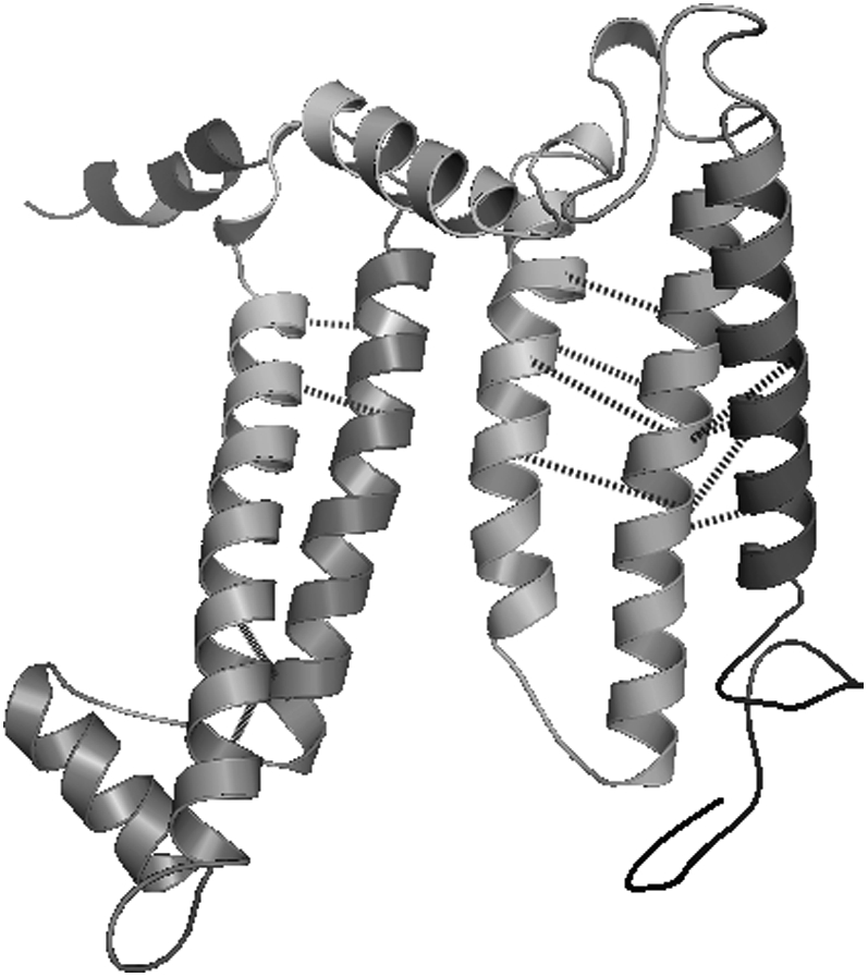
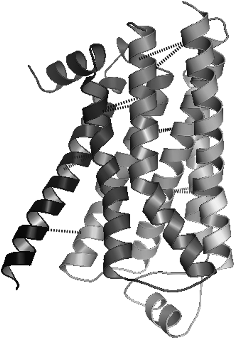
Bovine rhodopsin (1f88) is a well-known and well-studied membrane protein that consists of 348 amino acids and seven transmembrane helices that range in length from 21 to 39 amino acids. This membrane protein is classified as a G-protein-coupled receptor in that it is activated by light and turns on the signaling pathway that allows for vision. Bovine rhodopsin has been crystallized with a resolution of 2.8 Å (43). Further studies of bovine rhodopsin have determined the structure with a better resolution (44), in the trigonal crystal form (45), and for a photoactivated intermediate structure (46). Both the pairwise and triplet contact prediction models are applied to bovine rhodopsin using a subtract parameter range of 0–3 and a max_contact range of 1–2 to generate 20 contact predictions. The best average contact distances for iteration thresholds of 5, 10, and 20 are presented in Table 4. One of the optimal contact predictions using the MIN-2 probability set and the triplet model with a max_contact parameter value of 2 and a subtract parameter value of 1 is shown in Table 6. This prediction has an average contact distance of 11.13 Å for 20 interhelical residue pairs. This predicted set of contacts is illustrated on the crystal structure in Fig. 11. The largest distances in this contact prediction are between helices 3 and 4 (Fig. 11, both in green), which partially results from the placement of these helices in a crisscrossed arrangement in the bundle. The ensemble of contact predictions for bovine rhodopsin, like the predictions for the protein 1h2sA, contain a large number of low average contact distance results. This observation is especially true for applications of the triplet model with both probability sets.

TABLE 6.

An optimal set of contact predictions for bovine rhodopsin (1f88A) using the triplet model and the MIN-2 probability set

Three-body contact	Three-body distances (Å)	Helix pair
(40L,41A)-292A	11.2,14.0	1-7
49M-(299A,300V)	11.1,11.1	1-7
(80A,81V)-124A	10.2,11.0	2-3
117A-(167C,168A)	11.5,9.0	3-4
132A-(152H,153A)	13.9,12.8	3-4
(163M,164A)-207M	10.8,10.5	4-5
(215P,216L)-257M	14.0,12.6	5-6
(253M,254V)-308M	9.6,12.5	6-7
(271V,272A)-288M	6.9,7.7	6-7

FIGURE 11.

An optimal set of contact predictions for bovine rhodopsin using the triplet model and the MIN-2 probability set.

As one of the largest protein systems studied, the complexity of the mixed-integer linear optimization model that must be solved for bovine rhodopsin (1f88-A) is described in further detail here. The largest of the models is the pairwise contact prediction model with the AL-P probability set, resulting in a model with 3368 binary variables and 170,934 constraints. Despite the large size of this model, it can be solved to optimality in 87 seconds using the CPLEX solver (Ver. 9.1) on a 3.2-GHz Intel Pentium 4 processor. The resulting complexity of the two interhelical contact models paired with the probability sets are presented in Data S1 as Table S3. Due to the limited number of membrane protein structures available for probability set development, the triplet models have fewer binary variables. This number is likely to increase (as the number of nonzero probability values increase) when more membrane protein structures become available.

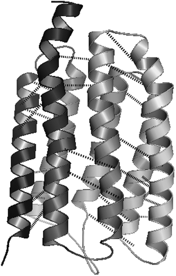
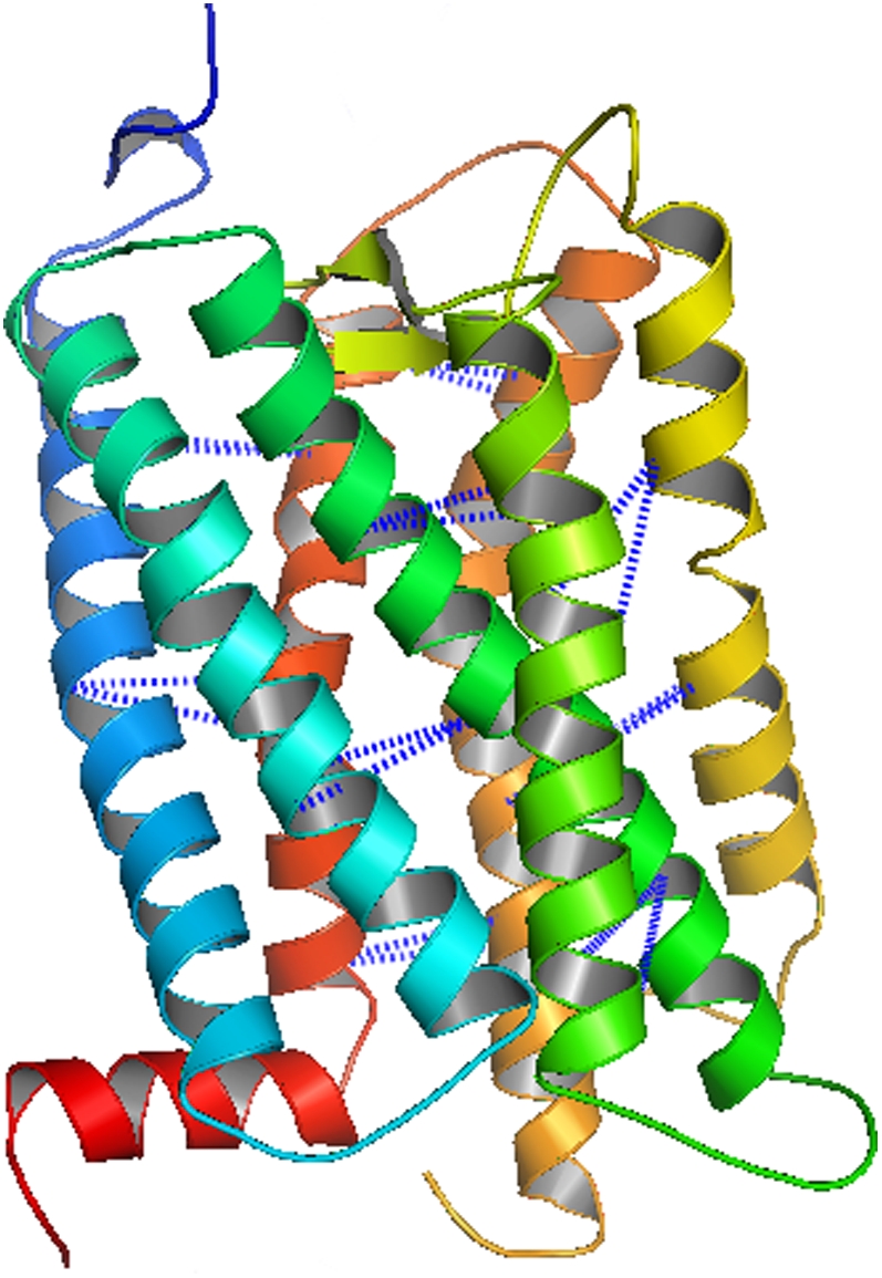
The proposed optimization models have also been validated by considering additional protein systems. One such system is the recently studied human β2 adrenergic receptor, a membrane protein with seven transmembrane α-helices. Two teams of researchers have succeeded in crystallizing this G-protein-coupled receptor by stabilizing the third inside loop (47,48). This protein was not available when the original protein data set was constructed and shares no significant sequence similarity to the other proteins in the data set. Both the pairwise and triplet contact prediction models are applied to this novel protein structure using a subtract parameter range of 0–3 and a max_contact range of 1–2 to generate 20 contact predictions. The best average contact distances for an iteration threshold of 20 and a variety of max_contact and subtract parameter values are presented in Table 7 after the proposed methodology is applied. Regardless of the parameter values and probability sets selected, a best average contact distance value of <14 Å is always identified for the human β2 adrenergic receptor protein. Table 8 highlights one high-scoring set of contact predictions with the triplet model and the AL-T probability set. This prediction has an average contact distance of 9.87 Å and is shown in Fig. 12.

TABLE 7.

The best average contact distances (in Å) of the human β2 adrenergic receptor protein predictions using four probability sets and a variety of parameterizations

max_contact	subtract	Pair MIN-1	Pair AL-P	Trip MIN-2	Trip AL-T
1	0	12.90	12.31	12.09	9.87
1	1	10.34	11.30	11.04	10.77
1	2	9.78	11.50	11.03	10.45
1	3	9.04	12.07	11.49	9.69
2	0	12.78	13.56	12.90	1l.72
2	1	13.57	13.73	12.84	12.13
2	2	13.04	11.65	12.26	11.40
2	3	10.48	12.88	11.75	11.13

TABLE 8.

A set of contact predictions for the human β2 adrenergic receptor protein using the triplet model and the AL-T probability set

Three-body contact	Three-body distances (Å)	Helix pair
37G-(90G,91A)	11.4,7.6	1-2
(45L,46A)-320G	9.1,6.0	1-7
(75L,76A)-124L	7.6,11.2	2-3
115L-(162G,163L)	5.9,8.9	3-4
167L-(202A,203S)	13.5,11.2	4-5
226A-(271A,272L)	11.0,8.4	5-6
(275L,276G)-324L	12.3,14.1	6-7

FIGURE 12.

A set of contact predictions for the human β2 adrenergic receptor protein using the triplet model and the AL-T probability set.

SUMMARY AND DISCUSSION

The results of applying the two novel optimization models of the section Pairwise Contact Prediction Model and the section following it, Triplet Contact Prediction Model, to the set of seven test systems are quite promising. The best average contact distance values consistently fall between 8.0 and 12.0 Å for six of these seven systems. The performance of the contact predictions for the three largest protein systems, 1h2sA, 1f88A, and 2rh1A, is particularly impressive. The results of the contact predictions for the test set do not clearly suggest that one probability set or one optimization model should be used in favor of another. Although further study is still required, the triplet model with the MIN-2 probability set may be the best choice currently available for a blind prediction of interhelical contacts in membrane proteins. Several of the contact predictions, including the prediction for 1zoyD with the triplet model and the MIN-2 probability set, appear to be limited by the small size of the data set used in the section Construction of a Data Set. The probability sets based on the contact type distributions identified by Liang and co-workers would also likely benefit from a larger set of membrane proteins with known structures.

The contact predictions presented here represent only a small fraction of the number of contacts that exist in a membrane protein. If two neighboring transmembrane proteins are perfectly parallel or antiparallel, several residue contacts exist at each helical turn. Of these 20–30 contacts that may exist between a pair of consecutive transmembrane helices, we aim to accurately predict 2–4 of the closest contacts and sacrifice coverage of all existing contacts. Due to the restricted conformation of α-helices, much of the information gained from additional contact predictions would be redundant for structure prediction efforts. An important area of future research is to use the information gained from this contact prediction model to predict the interhelical contacts among all helical pairs in the transmembrane bundle.

CONCLUSIONS

The problem of interhelical contact prediction in membrane proteins with transmembrane helices was addressed by

1. The construction of a nonredundant data set of membrane proteins.

2. The development of interhelical contact probabilities.

3. The application of mixed-integer linear programming models to identify the most probable set of interhelical contacts subject to a number of constraints.

These approaches were divided into the maximization of the most probable pairwise contacts and the maximization of the most probable three-body contacts. A two-stage optimization model was proposed for the prediction of pairwise interhelical contacts, where PRIMARY contacts are predicted first and WHEEL contacts are subsequently identified in a second stage. The alternative approach maximizes the probability of three-body interhelical contacts using a modification of the pairwise model. The proposed approach is shown to successfully predict interhelical contacts in seven membrane protein systems, including bovine rhodopsin and the recently released human β2 adrenergic receptor protein structure.

The importance of computational prediction methods for membrane proteins is underscored by the limitations of current experimental structure determination methods. Despite the success of the proposed methodology, further investigation into methods for developing interhelical contact probabilities should be explored to ensure the proposed optimization models perform up to their potential.

SUPPLEMENTARY MATERIAL

To view all of the supplemental files associated with this article, visit www.biophysj.org.

References

- 1.Berman, H. M., J. Westbrook, Z. Feng, G. Gilliland, T. N. Bhat, H. Weissig, I. N. Shindyalov, and P. E. Bourne. 2000. The Protein Data Bank. Nucleic Acids Res. 28:235–242. [DOI] [PMC free article] [PubMed] [Google Scholar]
- 2.Jayasinghe, S., K. Hristova, and S. H. White. 2000. MPTopo: a database of membrane protein topology. Protein Sci. 10:455–458. [DOI] [PMC free article] [PubMed] [Google Scholar]
- 3.Krogh, A., B. Larsson, G. von Heijne, and E. L. L. Sonnhammer. 2001. Predicting transmembrane protein topology with a hidden Markov model: applications to complete genomes. J. Mol. Biol. 157:105–132. [DOI] [PubMed] [Google Scholar]
- 4.Wallin, E., and G. von Heijne. 1998. Genome-wide analysis of integral membrane proteins from eubacterial, archaean, and eukaryotic organisms. Protein Sci. 7:1029–1038. [DOI] [PMC free article] [PubMed] [Google Scholar]
- 5.Hopkins, A. L., and C. R. Groom. 2002. The druggable genome. Nat. Rev. Drug Discov. 1:727–730. [DOI] [PubMed] [Google Scholar]
- 6.Jones, D. T., W. R. Taylor, and J. M. Thornton. 1994. A model recognition approach to the prediction of all-helical membrane protein structure and topology. Biochemistry. 33:3038–3049. [DOI] [PubMed] [Google Scholar]
- 7.Möller, S., M. D. R. Croning, and R. Apweiler. 2001. Evaluation of methods for the prediction of membrane spanning regions. Bioinformation. 17:646–653. [DOI] [PubMed] [Google Scholar]
- 8.Ikeda, M., M. Arai, D. M. Lao, and T. Shimizu. 2002. Transmembrane topology prediction methods: a reassessment and improvement by a consensus method using a dataset of experimentally characterized transmembrane topologies. In Silico Biol. 2:19–33. [PubMed] [Google Scholar]
- 9.Viklund, H., and A. Elofsson. 2004. Best α-helical transmembrane protein topology predictions are achieved using hidden Markov models and evolutionary information. Protein Sci. 13:1908–1917. [DOI] [PMC free article] [PubMed] [Google Scholar]
- 10.Zheng, W. J., V. Z. Spassov, L. Yan, P. K. Flook, and S. Szalma. 2004. A hidden Markov model with molecular mechanics energy-scoring function for transmembrane helix prediction. Comput. Biol. Chem. 28:265–274. [DOI] [PubMed] [Google Scholar]
- 11.Yuan, Z., J. S. Mattick, and R. D. Teasdale. 2004. SVMtm: support vector machines to predict transmembrane segments. J. Comput. Chem. 25:632–636. [DOI] [PubMed] [Google Scholar]
- 12.Xia, J.-X., M. Ikeda, and T. Shimizu. 2004. ConPred_elite: a highly reliable approach to transmembrane topology prediction. Comput. Biol. Chem. 28:51–60. [DOI] [PubMed] [Google Scholar]
- 13.Arkin, I. T., and A. T. Brunger. 1998. Statistical analysis of predicted transmembrane α-helices. Biochim. Biophys. Acta. 1429:113–128. [DOI] [PubMed] [Google Scholar]
- 14.Eilers, M., S. C. Shekar, T. Shieh, S. O. Smith, and P. J. Fleming. 2000. Internal packing of helical membrane proteins. Proc. Natl. Acad. Sci. USA. 97:5796–5801. [DOI] [PMC free article] [PubMed] [Google Scholar]
- 15.Eilers, M., A. B. Patel, W. Liu, and S. O. Smith. 2002. Comparison of helix interactions in membrane and soluble α-bundle proteins. Biophys. J. 82:2720–2736. [DOI] [PMC free article] [PubMed] [Google Scholar]
- 16.Adamian, L., and J. Liang. 2001. Helix-helix packing and interfacial pairwise interactions of residues in membrane proteins. J. Mol. Biol. 311:891–907. [DOI] [PubMed] [Google Scholar]
- 17.Bowie, J. 1997. Helix packing in membrane proteins. J. Mol. Biol. 272:780–789. [DOI] [PubMed] [Google Scholar]
- 18.Adamian, L., R. Jackups, Jr., T. A. Binkowski, and J. Liang. 2003. Higher-order interhelical spatial interactions in membrane proteins. J. Mol. Biol. 327:251–272. [DOI] [PubMed] [Google Scholar]
- 19.Gimpelev, M., L. R. Forrest, D. Murray, and B. Honig. 2004. Helical packing patterns in membrane and soluble proteins. Biophys. J. 87:4075–4086. [DOI] [PMC free article] [PubMed] [Google Scholar]
- 20.Wendel, C., and H. Gohlke. 2008. Predicting transmembrane helix pair configurations with knowledge-based distance-dependent pair potentials. Prot. Struct. Funct. Bioinf. 70:984–999. [DOI] [PubMed] [Google Scholar]
- 21.Waldispül, J., and J.-M. Steyaert. 2005. Modeling and predicting all-α transmembrane proteins including helix-helix pairing. Theor. Comput. Sci. 335:67–92. [Google Scholar]
- 22.Faulon, J.-L., K. Sale, and M. Young. 2003. Exploring the conformational space of membrane protein folds matching distance constraints. Protein Sci. 12:1750–1761. [DOI] [PMC free article] [PubMed] [Google Scholar]
- 23.Sale, K., J.-L. Faulon, G. A. Gray, J. S. Schoeniger, and M. Young. 2004. Optimal bundling of transmembrane helices using sparse distance constraints. Protein Sci. 13:2613–2627. [DOI] [PMC free article] [PubMed] [Google Scholar]
- 24.Chen, C.-M., and C.-C. Chen. 2003. Computer simulations of membrane protein folding: structure and dynamics. Biophys. J. 84:1902–1908. [DOI] [PMC free article] [PubMed] [Google Scholar]
- 25.Popot, J.-L., and D. M. Engelman. 1990. Membrane protein folding and oligomerization—the two-stage model. Biochemistry. 29:4031–4037. [DOI] [PubMed] [Google Scholar]
- 26.White, S. H., and W. C. Wimley. 1999. Membrane protein folding and stability: physical principles. Annu. Rev. Biophys. Biomol. Struct. 28:319–365. [DOI] [PubMed] [Google Scholar]
- 27.Vaidehi, N., W. B. Floriano, R. Trabanino, S. E. Hall, P. Freddolino, E. J. Choi, G. Zamanakos, and W. A. Goddard III. 2002. Prediction of structure and function of G protein-coupled receptors. Proc. Natl. Acad. Sci. USA. 99:12622–12627. [DOI] [PMC free article] [PubMed] [Google Scholar]
- 28.Becker, O. M., S. Shacham, Y. Marantz, and S. Noiman. 2003. Modeling the 3D structure of GPCRs: advances and application to drug discovery. Curr. Opin. Drug Discov. Devel. 6:353–361. [PubMed] [Google Scholar]
- 29.Shacham, S., Y. Marantz, S. Bar-Haim, O. Kalid, D. Warshaviak, N. Avisar, B. Inbal, A. Heifetz, M. Fichman, M. Topf, Z. Naor, S. Noiman, and O. M. Becker. 2004. PREDICT modeling and in-silico screening for G-protein coupled receptors. Prot. Struct. Funct. Bioinf. 57:51–86. [DOI] [PubMed] [Google Scholar]
- 30.Kim, S., A. K. Chamberlain, and J. U. Bowie. 2003. A simple method for modeling transmembrane helix oligomers. J. Mol. Biol. 329:831–840. [DOI] [PubMed] [Google Scholar]
- 31.Fleishman, S. J., and N. Ben-Tal. 2002. Conformations of tightly packed pairs of transmembrane α-helices. J. Mol. Biol. 321:363–378. [DOI] [PubMed] [Google Scholar]
- 32.Zhang, Y., M. E. Devries, and J. Skolnick. 2006. Structure modeling of all identified G protein-coupled receptors in the human genome. PLoS Comput. Biol. 2:e13. [DOI] [PMC free article] [PubMed] [Google Scholar]
- 33.Wang, G., and R. L. Dunbrack. 2003. PISCES: a protein sequence culling server. Bioinformation. 19:1589–1591. [DOI] [PubMed] [Google Scholar]
- 34.Choma, C., H. Gratkowski, J. D. Lear, and W. F. DeGrado. 2000. Asparagine mediate self-association of a model transmembrane helix. Nat. Struct. Biol. 7:161–166. [DOI] [PubMed] [Google Scholar]
- 35.Zhou, F. X., M. J. Cocco, W. P. Russ, A. T. Brunger, and D. M. Engelman. 2000. Interhelical hydrogen bonding drives strong interactions in membrane proteins. Nat. Struct. Biol. 7:154–160. [DOI] [PubMed] [Google Scholar]
- 36.Livingstone, J. R., R. S. Spolar, and M. T. Record, Jr. 1991. Contribution to the thermodynamics of protein folding from the reduction in water-accessible nonpolar surface area. Biochemistry. 30:4237–4244. [DOI] [PubMed] [Google Scholar]
- 37.McAllister, S. R., B. E. Mickus, J. L. Klepeis, and C. A. Floudas. 2006. A novel approach for α-helical topology prediction in globular proteins: generation of interhelical restraints. Prot. Struct. Funct. Bioinf. 65:930–952. [DOI] [PubMed] [Google Scholar]
- 38.Floudas, C. A. 1995. Nonlinear and Mixed-Integer Optimization: Fundamentals and Applications. Oxford University Press, Oxford, UK.
- 39.Brooke, A., D. Kendrick, A. Meeraus, and R. Raman. 2003. GAMS: A User's Guide. GAMS Development Corporation, South San Francisco, CA.
- 40.ILOG. 2003. CPLEX User's Manual 9.0. ILOG, Sunnyvale, CA and Genilly, France.
- 41.Dash Optimization. 2003. Xpress-MP: Getting Started. Dash Optimization, Englewood Cliffs, NJ.
- 42.Gordeliy, V. I., J. Labahn, R. Moukhametzianov, R. Efremov, J. Granzin, R. Schlesinger, G. Büldt, T. Savopol, A. J. Scheidig, J. P. Klare, and M. Engelhard. 2002. Molecular basis of transmembrane signaling by sensory rhodopsin II-transducer complex. Nature. 419:484–487. [DOI] [PubMed] [Google Scholar]
- 43.Palczewski, K., T. Kumasaka, T. Hori, C. A. Behnke, H. Motoshima, B. A. Fox, I. Le Trong, D. C. Teller, T. Okada, R. E. Stenkamp, M. Yamamoto, and M. Miyano. 2000. Crystal structure of rhodopsin: a G protein-coupled receptor. Science. 289:739–745. [DOI] [PubMed] [Google Scholar]
- 44.Okada, T., M. Sugihara, A.-N. Bondar, M. Elstner, P. Entel, and V. Buss. 2004. The retinal conformation and its environment in rhodopsin in light of a new 2.2 Å crystal structure. J. Mol. Biol. 342:571–583. [DOI] [PubMed] [Google Scholar]
- 45.Li, J., P. C. Edwards, M. Burghammer, C. Villa, and G. F. X. Schertler. 2004. Structure of bovine rhodopsin in a trigonal crystal form. J. Mol. Biol. 343:1409–1438. [DOI] [PubMed] [Google Scholar]
- 46.Salom, D., D. T. Lodowski, R. E. Stenkamp, I. Le Trong, M. Golczak, B. Jastrzebska, T. Harris, J. A. Ballesteros, and K. Palczewski. 2006. Crystal structure of a photoactivated deprotonated intermediate of rhodopsin. Proc. Natl. Acad. Sci. USA. 103:16123–16128. [DOI] [PMC free article] [PubMed] [Google Scholar]
- 47.Cherezov, V., D. M. Rosenbaum, M. A. Hanson, S. G. F. Rasmussen, F. S. Thian, T. S. Kobilka, H.-J. Choi, P. Kuhn, W. I. Weis, B. K. Kobilka, and R. C. Stevens. 2007. High-resolution crystal structure of an engineered human β2-adrenergic G protein-coupled receptor. Science. 318:1258–1265. [DOI] [PMC free article] [PubMed] [Google Scholar]
- 48.Rasmussen, S. G. F., H.-J. Choi, D. M. Rosenbaum, T. S. Kobilka, F. S. Thian, P. C. Edwards, M. Burghammer, V. R. P. Ratnala, R. Sanishvili, R. F. Fischetti, G. F. X. Schertler, W. I. Weis, and B. K. Kobilka. 2007. Crystal structure of the human β2 adrenergic G-protein-coupled receptor. Nature. 450:383–387. [DOI] [PubMed] [Google Scholar]
- 49.DeLano, W. L. 2002. The PyMol Molecular Graphics System. DeLano Scientific, Palo Alto, CA. http://www.pymol.org.
Associated Data
This section collects any data citations, data availability statements, or supplementary materials included in this article.