Fitting Computational Models to fMRI Data

Abstract

Many computational models in psychology predict how neural activation in specific brain regions should change during certain cognitive tasks. The emergence of fMRI as a research tool provides an ideal vehicle to test these predictions. Before such tests are possible, however, significant methodological problems must be solved. These problems include transforming the neural activations predicted by the model into predicted BOLD responses, identifying the voxels within each region of interest against which to test the model, and comparing the observed and predicted BOLD responses in each of these regions. Methods are described for solving each of these problems.

INTRODUCTION

Functional magnetic resonance imaging (fMRI) has revolutionized Psychology. The effects have probably been greatest within Cognitive Psychology and Perception, but the influence of fMRI has spread to almost every area of Psychology. For example, there are now emerging new fields of Social Neuroscience, Developmental Neuroscience, and Neuroeconomics, all largely due to fMRI. There is even a new field of Neuromarketing. By far, the great majority of fMRI research in these fields uses fMRI as a tool for exploratory research. The most common question in this approach is: Which brain areas are activated by the task I am studying? This is clearly an important question that has had enormous benefit and will continue to do so in the future.

On the other hand, we believe fMRI has significant untapped potential as a tool for confirmatory research. In such an approach, the research question instead would be: Does a model or theory correctly predict the results of an fMRI experiment? Or alternatively, which of two competing models gives the best account of fMRI data? Requiring that a satisfactory model is consistent not only with available behavioral data but also with fMRI data greatly constrains the class of acceptable models. In most cognitive behavioral experiments, at best only two pieces of behavioral data are available on each trial - which response was made and the response time. Many models that postulate qualitatively different underlying psychological processes might nevertheless give equally good accounts of such sparse data sets. In contrast, fMRI data is incredibly rich, and the class of models that are consistent with both the behavioral and fMRI data is likely to be quite small.

It is true that models potentially capable of making predictions about the outcome of fMRI experiments must make neurobiological assumptions that may not be necessary if the goal is to account simply for behavioral data. Even so, there are now many neurobiologically detailed computational models in Psychology that make predictions (or could make predictions) about how neural activity changes in specific brain regions as participants perform certain cognitive tasks, and fMRI seems ideally suited to testing such predictions (e.g., Anderson & Qin, in press; Ashby, Ell, Valentin, & Casale, 2005; Brown & Braver, 2005; Chadderdon & Sporns, 2006; Frank & Claus, 2006; Mason & Just, 2006; Monchi, Taylor, & Dagher, 2000; O’Reilly, 2006).

Yet to test computational models in this way, several problems must be overcome. First, psychological models might make predictions about neural activation, but they generally do not make predictions about the blood-oxygen-level-dependent (BOLD) signal that is most commonly measured in fMRI experiments. So the first problem is to generate predicted BOLD responses from the model’s predicted neural activations.

Second, most models in Psychology that make neuroanatomical predictions typically do not make predictions that are specific enough to identify a small set of voxels in the region of interest (ROI) that could be used to test the model. For example, a model might specify that during a certain period of a working memory task, a specific type of activation should occur in dorsolateral prefrontal cortex (dlPFC). But such a model would generally not predict that every voxel in dlPFC would show this activation pattern - only that some would. So a second significant problem that must be solved is to identify exactly which voxels within dlPFC should be used to test the model. Finally, the third problem is to compare the observed and predicted BOLD responses in the selected voxels, and to decide on the basis of this comparison if the model succeeds or fails at accounting for the results of the experiment.

This article proposes solutions to these three problems. The solutions are straightforward and use standard fMRI statistical methods. There have been a few previous attempts to fit computational models to fMRI data (e.g., Danker & Anderson, 2007), and these have used some of the same methods proposed here (e.g., convolution with a hemodynamic response function). However, we know of no attempts that used all of the methods described below, nor do we know of any other articles that are devoted solely to this topic.

AN EXAMPLE

As an example of a model that could be tested against fMRI data, we will consider a recent computational model, called SPEED (Subcortical Pathways Enable Expertise Development), which describes how automaticity develops in perceptual categorization tasks (Ashby, Ennis, & Spiering, 2007). Briefly, the model assumes there are two neural pathways from the sensory association area that mediates perception of the stimulus to the premotor region of cortex that mediates response selection. A longer and slower path projects to the premotor area via the striatum, globus pallidus, and thalamus. A faster, purely cortical path projects directly from the sensory association area to the premotor area. SPEED assumes that the subcortical path, although slower, has greater neural plasticity because of a dopamine-mediated learning signal from the substantia nigra. In contrast, the faster cortical-cortical path learns more slowly via (dopamine independent) classical two-factor Hebbian learning. Because of its greater plasticity, early performance is dominated by the subcortical path, but the development of automaticity is characterized by a transfer of control to the faster cortical-cortical projection. The model includes differential equations that describe activation in each of the relevant brain areas as well as a set of difference equations that describe the relevant two- and three-factor learning.

Ashby et al. (2007) showed that SPEED accounts for some classic single-cell recording and behavioral results, but the model has not yet been tested against fMRI data. Even so, it makes detailed predictions about many of the brain regions that should show task-related activation during category learning. For example, SPEED predicts how neural activation in a variety of brain regions should change over the course of a single trial, and how these activations will change after many days of practice on the task. So fMRI seems like an ideal tool for rigorously testing the model.

PROBLEM 1: GENERATE BOLD PREDICTIONS FROM THE MODEL

The fMRI BOLD response increases with the amount of oxygenated hemoglobin in a voxel relative to the amount of de-oxygenated hemoglobin (Ogawa, Lee, Kay, & Tank, 1990). Compared to the neural activation that presumably drives it, the BOLD response is highly sluggish. It reaches a peak around 6 sec after the neural activation that induced it, and slowly decays back to baseline 20 - 25 sec later. The first step in fitting a neurocomputational model to fMRI data therefore, is to convert the predicted neural activations into predicted BOLD responses.

Almost all current applications of fMRI assume that the transformation from neural activation to BOLD response can be modeled as a linear, time-invariant system (e.g., Boynton, Engel, Glover, & Heeger, 1996). In the linear systems approach, one can conceive of the vascular system that responds to a sudden oxygen debt as a black box in which the input is neural activation and the output is the BOLD response. Suppose we present a stimulus event E_i to a subject at time 0. Let N_i(t) denote the neural activation induced by this event at time t, and let B(t) denote the resulting BOLD response. A system of this type is linear if and only if

$$\mathrm{B}[{\mathrm{N}}_1\left(t\right)+{\mathrm{N}}_2\left(t\right)]=\mathrm{B}\left[{\mathrm{N}}_1\left(t\right)\right]+\mathrm{B}\left[{\mathrm{N}}_2\left(t\right)\right].$$

If the system is linear, then it is well known that the BOLD response to any neural activation N_i(t) can be computed from

$$\mathrm{B}\left(t\right)={\int }_0^t\mathrm{N}\left(\tau \right)\mathrm{h}(t-\tau )d\tau .$$ (1)

Equation 1 is the well-known convolution integral that completely characterizes the behavior of any linear, time-invariant system (e.g., Chen, 1970). The function h(t) is traditionally called the impulse response function because it describes the response of the system to an input that is a perfect impulse. In the fMRI literature however, h(t) is known as the hemodynamic response function, often abbreviated as the hrf. The hrf is the hypothetical BOLD response to an idealized impulse of neural activation, often peaking at 6 sec and lasting for 30 secs or so.

To generate a predicted BOLD response from our model, we first use the model to generate a predicted neural response N(t). For example, the top panel of Figure 1 shows the neural activation predicted by SPEED (Ashby et al., 2007) in premotor cortex (i.e., either supplementary motor area or pre-supplementary motor area) during one categorization trial and after 50 trials of practice. In this example, the trial begins with a 1 sec fixation period.

Figure 1.

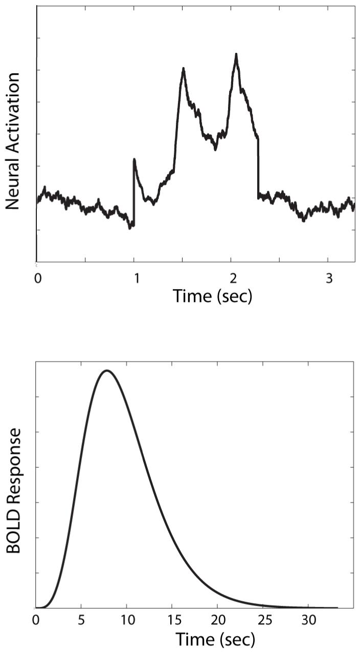
The top panel shows activation predicted by the computational model SPEED (Ashby et al., 2007) in premotor cortex during a single categorization trial. The bottom panel shows the predicted BOLD response under these same conditions.

The next step is to select a mathematical form for the hrf. These two functions are then numerically convolved (via Eq. 1) to produce a predicted BOLD response. There are many alternative models of the hrf. A common approach is to select a canonical form for the hrf that is characterized by several free parameters that can be adjusted to account for differences in the hrf across brain regions or subjects. Many alternative models of this type have been proposed (Boynton et al., 1996; Clark, Maisog, & Haxby, 1998; Cohen, 1997; Dale & Buckner, 1997; Friston, Holmes, & Ashburner, 1999; Friston, Josephs, Ress, & Turner, 1998; Zarahn, Aquirre, & D’Esposito, 1997). For example, Boynton et al. (1996) proposed a gamma function of the type

$$h\left(t\right)=\{\begin{array}{cc}\frac{{(t-T_0)}^{n-1}}{{\lambda }^n(n-1)!}{e}^{\frac{t-T_0}{\lambda }}\hfill & \text{for}t>T_0\hfill \\ 0\hfill & \text{for}t<T_0\hfill \end{array}\phantom{\}}$$ (2)

where λ, T₀, and n (an integer) are free parameters. The parameter T₀ is the lag between stimulus presentation and the initial rise in the BOLD response, whereas λ and n determine the shape of the hrf. For example, the peak of the hrf occurs at time T₀ + (n - 1)λ. The parameters can either be estimated from the data or else just set to some typical values. Figure 2 shows an example of this model with the parameters set to T₀ = 0, n = 4, and λ = 2. The bottom panel of Figure 1 shows the result of convolving the Figure 1 neural activation predicted by SPEED (top panel) with the hrf shown in Figure 2. This is the BOLD response predicted by SPEED in this particular ROI for one categorization trial.

Figure 2.

A typical hrf used in fMRI data analysis. This is the gamma function model of Eq. 2 that was proposed by Boynton et al. (1996) with T₀ = 0, n = 4, and λ = 2.

All models of the hrf have the same basic shape, in the sense that they all rise to a peak at around 6 seconds and then slowly decay back to baseline. Some include a late negative dip because empirical estimates of the BOLD response often show this property (e.g., Fransson, Kruger, Merboldt, & Frahm, 1999; Glover, 1999). All models, however, that use an hrf to predict a BOLD response via the Eq. 1 convolution integral, depend critically on the linearity assumption. There is good evidence that linearity is approximately satisfied if the time between stimulus events exceeds several seconds and if brief stimulus exposure durations are avoided (Vazquez & Noll, 1998). However, if stimulus events quickly follow one another, or if brief stimulus exposure durations are used, then it is well documented that the BOLD response exhibits significant nonlinearities (Hinrichs et al., 2000; Huettel, & McCarthy, 2000; Ogawa et al., 2000; Pfeuffer, McCullough, Van de Moortele, Ugurbil, & Hu, 2003). In this case, Eq. 1 is no longer valid. Some complex approaches directly model the physical processes that cause these nonlinearities (e.g., the balloon model of Buxton, Wong, & Frank, 1998). Alternatively, Friston et al. (1998) proposed a computationally simpler method that uses a second order Volterra series for modeling nonlinearities that simply adds a correction term to Eq. 1.

In summary, there is a large literature on alternative methods for modeling the BOLD response (for a review, see e.g., Henson & Friston, 2007). The simplest solution is to use a model of the hrf with no free parameters. An intermediate choice is to use an hrf model that has free parameters that must be estimated from the data. A third, more sophisticated choice, is to replace the hrf with a second order Volterra series that models nonlinearities in the transformation from neural activation to BOLD response. The decision about which of these solutions to choose should depend on the experimental design, the amount of detail specified by the computational model to be tested, and on the state of the field within which that model resides. For example, the decision about whether to use linear (i.e., hrf) or nonlinear (e.g., Volterra series) methods should depend on whether the experiment used brief stimulus exposures and short inter-stimulus intervals. As another example, a parameter-free model of the hrf might suffice in research areas where there have been no previous attempts to fit computational models to fMRI data.

PROBLEM 2: IDENTIFY VOXELS AGAINST WHICH TO TEST THE MODEL

Once predicted BOLD responses have been generated from the model, the second problem is to identify exactly which voxels should be used to provide the data that the model will be tested against. Our solution to this problem includes three steps. The first is to apply the general linear model (GLM) to each voxel using the method of Ollinger, Shulman, and Corbetta (2001a, 2001b). The second step is to form a statistical parametric t-map (t-SPM) from these GLM results, and the third step is to identify the set of candidate voxels within each ROI from this SPM.

Step 1. Apply the GLM to each voxel using the method of Ollinger et al

Consider an fMRI experiment in which the time between onsets of successive whole brain scans (i.e., the repetition time or TR) is 3 seconds, and the BOLD response to a stimulus onset lasts for 12 seconds, or equivalently 5 TRs. This is an unrealistic value, since in most cases we would expect the BOLD response to last at least twice this long. However, this shorter value is sufficient to illustrate the computational method. Ollinger et al. (2001a, 2001b) proposed that in this case we define 5 different parameters that describe the BOLD response to the stimulus presentation at each of the ensuing 5 TRs. Call these 5 parameters β₁, β₂, β₃, β₄, and β₅. Assume also that every time the same stimulus is presented the exact same BOLD response occurs.

Now consider an event-related experimental design in which a stimulus event occurs on TRs 1, 3, 4, and 7. Then the stimulus events and their BOLD responses at each TR will be:

$$\begin{array}{ccccccccc}\hfill \mathrm{TR}:& \hfill 1\hfill & \hfill 2\hfill & \hfill 3\hfill & \hfill 4\hfill & \hfill 5\hfill & \hfill 6\hfill & \hfill 7\hfill & \hfill 8\dots \hfill \\ \hfill \text{Events}:& \hfill E\hfill & \hfill \hfill & \hfill E\hfill & \hfill E\hfill & \hfill \hfill & \hfill \hfill & \hfill E\hfill & \hfill \hfill \\ \hfill \text{BOLD response to}{1}^{\mathrm{st}}\text{event}:& \hfill {\beta }_1\hfill & \hfill {\beta }_2\hfill & \hfill {\beta }_3\hfill & \hfill {\beta }_4\hfill & \hfill {\beta }_{5\cdot }\hfill & \hfill \hfill & \hfill \hfill & \hfill \hfill \\ \hfill \text{BOLD response to}{2}^{\mathrm{nd}}\text{event}:& \hfill \hfill & \hfill \hfill & \hfill {\beta }_1\hfill & \hfill {\beta }_2\hfill & \hfill {\beta }_3\hfill & \hfill {\beta }_4\hfill & \hfill {\beta }_{5\cdot }\hfill & \hfill \hfill \\ \hfill \text{BOLD response to}{3}^{\mathrm{rd}}\text{event}:& \hfill \hfill & \hfill \hfill & \hfill \hfill & \hfill {\beta }_1\hfill & \hfill {\beta }_2\hfill & \hfill {\beta }_3\hfill & \hfill {\beta }_4\hfill & \hfill {\beta }_{5\cdot }\hfill \\ \hfill \text{BOLD response to}{4}^{\mathrm{th}}\text{event}& \hfill \hfill & \hfill \hfill & \hfill \hfill & \hfill \hfill & \hfill \hfill & \hfill \hfill & \hfill {\beta }_1\hfill & \hfill {\beta }_2\hfill \end{array}$$

Therefore, if the system is linear then the observed BOLD response at each TR will equal:

$$\begin{array}{cc}\hfill \underset{‒}{\mathrm{TR}}\hfill & \hfill \underset{‒}{\text{BOLD}}\hfill \\ \hfill 1\hfill & \hfill {\beta }_1\hfill \\ \hfill 2\hfill & \hfill {\beta }_2\hfill \\ \hfill 3\hfill & \hfill {\beta }_1+{\beta }_3\hfill \\ \hfill 4\hfill & \hfill {\beta }_1+{\beta }_2+{\beta }_4\hfill \\ \hfill 5\hfill & \hfill {\beta }_2+{\beta }_3+{\beta }_5\hfill \\ \hfill 6\hfill & \hfill {\beta }_3+{\beta }_4\hfill \\ \hfill 7\hfill & \hfill {\beta }_1+{\beta }_4+{\beta }_5\hfill \\ \hfill 8\hfill & \hfill {\beta }_2+{\beta }_5\hfill \end{array}$$

These equations can be expressed in terms of the GLM as follows:

$$\left[\begin{array}{c}\hfill \mathrm{B}\left(1\right)\hfill \\ \hfill \mathrm{B}\left(2\right)\hfill \\ \hfill \mathrm{B}\left(3\right)\hfill \\ \hfill \mathrm{B}4)\hfill \\ \hfill \mathrm{B}\left(5\right)\hfill \\ \hfill \mathrm{B}\left(6\right)\hfill \\ \hfill \mathrm{B}\left(7\right)\hfill \\ \hfill \mathrm{B}\left(8\right)\hfill \end{array}\right]=\left[\begin{array}{ccccccc}\hfill 1\hfill & \hfill 0\hfill & \hfill 0\hfill & \hfill 0\hfill & \hfill 0\hfill & \hfill 1\hfill & \hfill 1\hfill \\ \hfill 0\hfill & \hfill 1\hfill & \hfill 0\hfill & \hfill 0\hfill & \hfill 0\hfill & \hfill 1\hfill & \hfill 2\hfill \\ \hfill 1\hfill & \hfill 0\hfill & \hfill 1\hfill & \hfill 0\hfill & \hfill 0\hfill & \hfill 1\hfill & \hfill 3\hfill \\ \hfill 1\hfill & \hfill 1\hfill & \hfill 0\hfill & \hfill 1\hfill & \hfill 0\hfill & \hfill 1\hfill & \hfill 4\hfill \\ \hfill 0\hfill & \hfill 1\hfill & \hfill 1\hfill & \hfill 0\hfill & \hfill 1\hfill & \hfill 1\hfill & \hfill 5\hfill \\ \hfill 0\hfill & \hfill 0\hfill & \hfill 1\hfill & \hfill 1\hfill & \hfill 0\hfill & \hfill 1\hfill & \hfill 6\hfill \\ \hfill 1\hfill & \hfill 0\hfill & \hfill 0\hfill & \hfill 1\hfill & \hfill 1\hfill & \hfill 1\hfill & \hfill 7\hfill \\ \hfill 0\hfill & \hfill 1\hfill & \hfill 0\hfill & \hfill 0\hfill & \hfill 1\hfill & \hfill 1\hfill & \hfill 8\hfill \end{array}\right]\left[\begin{array}{c}\hfill {\beta }_1\hfill \\ \hfill {\beta }_2\hfill \\ \hfill {\beta }_3\hfill \\ \hfill {\beta }_4\hfill \\ \hfill {\beta }_5\hfill \\ \hfill B_0\hfill \\ \hfill \Delta \hfill \end{array}\right]+\left[\begin{array}{c}\hfill {\epsilon }_1\hfill \\ \hfill {\epsilon }_2\hfill \\ \hfill {\epsilon }_3\hfill \\ \hfill {\epsilon }_4\hfill \\ \hfill {\epsilon }_5\hfill \\ \hfill {\epsilon }_6\hfill \\ \hfill {\epsilon }_7\hfill \\ \hfill {\epsilon }_8\hfill \end{array}\right]$$ (3)

where B₀ estimates the baseline activation and Δ measures the amount of linear drift in the magnetic field strength. Jittering the stimulus events guarantees that X’X is nonsingular. Therefore, uniformly minimum variance unbiased estimators of β (i.e., the gold standard of parameter estimation) are computed from the solution of the GLM normal equations

$$\underset{‒}{\widehat{\beta }}={\left({\mathrm{X}}^{\prime }\mathrm{X}\right)}^{-1}{\mathrm{X}}^{\prime }\underset{‒}{\mathrm{y}}.$$ (4)

This GLM analysis is performed separately in every voxel. The end result is a $\underset{‒}{\widehat{\beta }}$ vector for every voxel. In the next step we will reduce each of these vectors to a single t statistic.

Step 2: Form the SPM

The SPM we will form compares the central ${\widehat{\beta }}_{\mathrm{i}}$ with the early and late ${\widehat{\beta }}_{\mathrm{i}}$. For example, if the BOLD response to an event is assumed to persist for 25 seconds and the TR is 2.5 seconds, then there will be 11 ${\widehat{\beta }}_{\mathrm{i}}$. In this case, we will construct the SPM that tests the null hypothesis

$${\mathrm{H}}_0:({\beta }_2+{\beta }_3+{\beta }_4)-({\beta }_1+{\beta }_{10}+{\beta }_{11})=0$$ (5)

against the alternative

$${\mathrm{H}}_1:({\beta }_2+{\beta }_3+{\beta }_4)-({\beta }_1+{\beta }_{10}+{\beta }_{11})>0.$$

Although SPMs based on other simpler hypotheses could be produced, this particular SPM has several attractive advantages. Most importantly, it uses more data than SPMs based on simpler hypotheses and it makes stronger structural assumptions. For example, the t-statistic produced from the Eq. 5 null hypothesis will be large only if the BOLD response starts small, grows to a large value between 2.5 and 7.5 seconds after the stimulus event, and then decays back to a small value by 22.5 seconds after the event.

Note that the null hypothesis specified by Eq. 5 can be written in matrix form as

$${\mathrm{H}}_0:{\underset{‒}{\mathrm{w}}}^{\prime }\underset{‒}{\beta }=0,$$

where w’ is the row vector

$${\underset{‒}{\mathrm{w}}}^{\prime }=[-111100000-1-100].$$

Note that the last two 0’s in this vector remove the influence of B₀ and Δ on the SPM. If, as is common, we assume homogeneity of variance and independence across TRs, then under this null hypothesis, the statistic

$$t=\frac{{\underset{‒}{\mathrm{w}}}^{\prime }\underset{‒}{\widehat{\beta }}}{\sqrt{{\widehat{\sigma }}^2{\underset{‒}{\mathrm{w}}}^{\prime }{\left({\mathrm{X}}^{\prime }\mathrm{X}\right)}^{-1}\underset{‒}{\mathrm{w}}}},$$ (6)

has a t distribution with degrees of freedom equal to

$$d{f}_E=\left(\#\text{of}\mathrm{TRs}\right)-1-\left(\#\text{of parameters in}\underset{‒}{\beta }\right).$$

The maximum likelihood estimator of σ² is known to equal:

$${\widehat{\sigma }}^2=\frac{1}{d{f}_E}{(\underset{‒}{y}-\mathrm{X}\underset{‒}{\widehat{\beta }})}^{\prime }(\underset{‒}{y}-\mathrm{X}\underset{‒}{\widehat{\beta }}).$$ (7)

We now have a single t-statistic in every voxel. Large values will come from voxels that appear to be task responsive.

Step 3: Select Voxels for Model Testing

The next step is to use the t-SPM to select the specific voxels within each ROI that will be used in the model testing. There are a number of plausible methods for achieving this goal. One possibility is to select the n voxels within each ROI that have the largest t-values. The value of n should probably increase with the size of the ROI, but for purposes of discussion a value of n = 10 is reasonable. One advantage of this method is that no statistical threshold is used to identify voxels. Thus, the 10 largest t-statistics in an area might all fall below the statistical threshold for significance. Presumably the model predicts that these t-values should all be significant, so by excluding a significance criterion from our selection procedure we are minimizing one important type of selection bias.

A disadvantage of this method is that the 10 voxels selected might not be contiguous. So another approach might be to use a cluster-based selection procedure, where a cluster is defined as a set of contiguous (supra-threshold) voxels. In this method, an intermediate threshold is set - for example, at T = 2.5 - after the t-map is formed in Step 2. Next, voxels with t-values greater than this threshold are used to identify all clusters in the ROI. Finally, within each ROI specified by the model, one might identify the largest cluster, and use data from these voxels to test the model.

At this point, there is no empirical rationale for choosing one of these methods over the other. Thus, the choice of which method is used should probably depend on the theoretical predictions of the model. For example, SPEED predicts that in a task with two response alternatives, there should be two separate task-sensitive striatal units. The model assumes that if the stimuli associated with each response are similar, and the motor actions required to produce each response are similar, then the two striatal units should be near each other in the striatum, but SPEED does not assume that they must be contiguous. For this reason, the method that chooses the n voxels with the largest t values is probably preferable to the method that chooses the largest above-threshold cluster.

PROBLEM 3: COMPARE OBSERVED AND PREDICTED BOLD RESPONSES IN SELECTED VOXELS

We are now in a position to address the last of our three problems. There are four steps to complete.

Step 1. Prepare the Data

In each ROI specified by the model, we have identified 10 voxels that we will use for model testing. In each voxel, a BOLD response was recorded at every TR of the experiment. Suppose that the experiment included a total of N TRs. Then the data from each of the selected voxels is an N × 1 vector. The first step is to compute the mean of the 10 selected data vectors in each ROI. After this averaging process, there will be one N × 1 data vector in each ROI. Our task is to generate a predicted vector from the model in each ROI and to compare the predicted vector with this observed data vector.

Step 2. Prepare the Model

The goal of this step is to produce an N × 1 vector containing predicted BOLD responses at each TR of the experiment. To begin, as described in the solution to Problem 1, the equations of the model are used to generate predicted neural activation in each ROI during every TR of the experiment. For example, the top panel of Figure 3 shows the neural activations predicted by SPEED in premotor cortex during the first 30 seconds of a hypothetical event-related fMRI experiment. In this example, the TR is 3 sec and a categorization stimulus is presented on TRs 1, 4, 5, 7, and 10. Each categorization TR begins with a 2 sec pause and ends with a 1 sec stimulus presentation.

Figure 3.

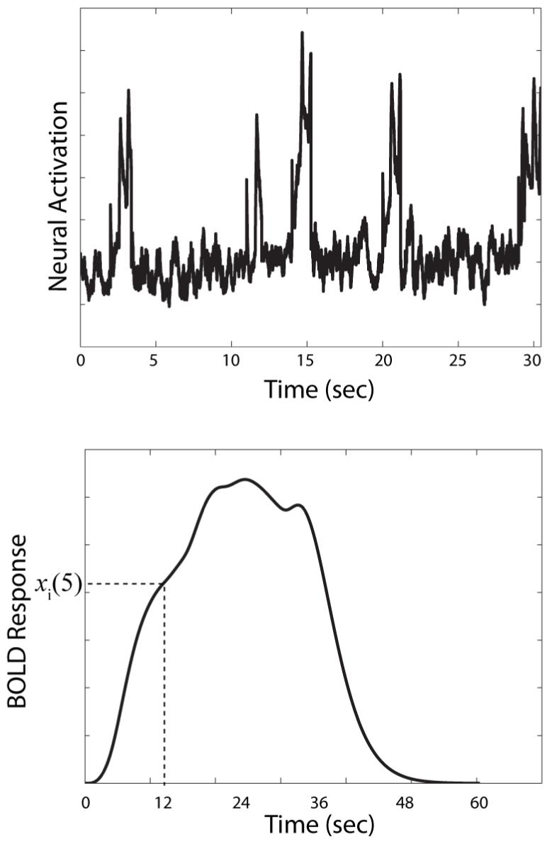
The top panel shows activation predicted by the computational model SPEED (Ashby et al., 2007) in premotor cortex during 30 seconds of an event-related fMRI experiment. The bottom panel shows the predicted BOLD response under these same conditions.

Next, these predicted neural activations are numerically convolved with an hrf to produce the predicted BOLD response at each ROI throughout the experiment. The bottom panel of Figure 3 shows the results of convolving the Figure 2 hrf with the neural activations shown in the top panel of Figure 3. This process is completed by filling an N × 1 vector (for every ROI) with the values of this predicted BOLD response at each of the N TRs of the experiment. Let x_i(1), x_i(2), ..., x_i(N) denote these predicted values in the ith ROI. The bottom panel of Figure 3 shows how the value x_i(5) is defined.

Finally, we build the following GLM at each ROI:

$$\left[\begin{array}{c}\hfill B_i\left(1\right)\hfill \\ \hfill B_i\left(2\right)\hfill \\ \hfill ⋮\hfill \\ \hfill B_i\left(N\right)\hfill \end{array}\right]=\left[\begin{array}{ccc}\hfill x_i\left(1\right)\hfill & \hfill 1\hfill & \hfill 1\hfill \\ \hfill x_i\left(2\right)\hfill & \hfill 1\hfill & \hfill 2\hfill \\ \hfill ⋮\hfill & \hfill ⋮\hfill & \hfill ⋮\hfill \\ \hfill x_i\left(N\right)\hfill & \hfill 1\hfill & \hfill N\hfill \end{array}\right]\left[\begin{array}{c}\hfill {\theta }_M\hfill \\ \hfill B_0\hfill \\ \hfill \Delta \hfill \end{array}\right]+\left[\begin{array}{c}\hfill {\epsilon }_1\hfill \\ \hfill {\epsilon }_2\hfill \\ \hfill ⋮\hfill \\ \hfill {\epsilon }_N\hfill \end{array}\right]$$ (8)

where θ_M measures the correlation between the predictions of the model and the data. As before, B₀ is the baseline activation and Δ measures the linear drift in the magnetic field strength.

If the model is correct then, of course, θ_M should be large. Equation 6 with

$${\underset{‒}{\mathrm{w}}}^{\prime }=\left[100\right]$$

can be used to test the null and alternative hypotheses

$${\mathrm{H}}_0:{\theta }_M=0$$

and

$${\mathrm{H}}_1:{\theta }_M>0.$$

Under this null hypothesis the Eq. 6 t-statistic has a t-distribution with df_E = N - 4. Thus, rejecting this null hypothesis in each ROI specified by the model is evidence that the model provides a good fit to the data from this experiment.

The use of the GLM to evaluate the fit of the model requires that no free parameters are estimated during the fitting process. One possibility is to estimate the free parameters in the model by first fitting to single-unit recording data (as in Ashby et al., 2005) or behavioral data. If free parameters in the model must be estimated from the fMRI data, then a traditional iterative minimization routine must be used instead of the GLM during this step (i.e., for parameter estimation and model fitting).

In general, the same is true if a model of the hrf is chosen that has free parameters that must be estimated from the data. Obviously, if a poor model of the hrf is chosen, the correlation between predicted and observed BOLD responses will be low, even if the model accurately predicts the neural activation. If an iterative estimation procedure is used to estimate parameters of the hrf then the convolution integral of Eq. 1 must be computed numerically at each iteration.

Friston et al. (1998) had a clever idea that eliminates most of this numerical integration. Their idea was to model the hrf as a weighted linear combination of basis functions:

$$h\left(t\right)={\theta }_1{b}_1\left(t\right)+{\theta }_2{b}_2\left(t\right)+{\theta }_3{b}_3\left(t\right),$$ (9)

where b_i(t) is the i^th basis function and θ_i is its weight. Friston et al. (1998) suggested gamma probability density functions for the b_i(t) with means and variances equal to 4, 8, and 16, respectively. The key though is that none of the b_i(t) have any free parameters. The only free parameters are the weights θ₁, θ₂, and θ₃.

The advantage of defining the hrf in terms of basis functions can be seen when Eq. 9 is substituted into the convolution integral of Eq. 1:

$$\begin{array}{cc}\hfill \mathrm{B}\left(t\right)& ={\int }_0^t\mathrm{N}\left(\tau \right)\mathrm{h}(t-\tau )d\tau \hfill \\ \hfill & ={\int }_0^t\mathrm{N}\left(\tau \right)[{\theta }_1{b}_1(t-\tau )+{\theta }_2{b}_2(t-\tau )+{\theta }_3{b}_3(t-\tau )]d\tau \hfill \\ \hfill & ={\theta }_1\left[{\int }_0^t\mathrm{N}\left(\tau \right){\mathrm{b}}_1(t-\tau )dt\right]+{\theta }_2\left[{\int }_0^t\mathrm{N}\left(\tau \right){\mathrm{b}}_2(t-\tau )dt\right]+{\theta }_3\left[{\int }_0^t\mathrm{N}\left(\tau \right){\mathrm{b}}_3(t-\tau )dt\right]\hfill \end{array}$$

Note that none of these integrals include any free parameters. As a result, if we define

$${\mathrm{y}}_i\left(t\right)={\int }_0^t\mathrm{N}\left(\tau \right){\mathrm{b}}_i(t-\tau )d\tau ,$$ (10)

then

$$\mathrm{B}\left(t\right)={\theta }_1{\mathrm{y}}_1\left(t\right)+{\theta }_2{\mathrm{y}}_2\left(t\right)+{\theta }_3{\mathrm{y}}_3\left(t\right),$$

where the only free parameters are the θ_i.

With this re-formulation of B(t), the iterative and time-consuming parameter estimation process can be avoided. Instead, optimal parameter estimates can be computed in one step. First, the three integrals specified in Eq. 10 are computed numerically. Each of these computations produces a vector of numerical values, y₁(t), y₂(t), and y₃(t). The parameters θ_i can now be determined using standard linear regression techniques. First, the vector x(t) in column 1 of the Eq. 8 design matrix is replaced by the three columns y₁(t), y₂(t), and y₃(t), and the β vector becomes

$$\underset{‒}{\beta }=\left[\begin{array}{c}\hfill {\theta }_1\hfill \\ \hfill {\theta }_2\hfill \\ \hfill {\theta }_3\hfill \\ \hfill {\mathrm{B}}_0\hfill \\ \hfill \Delta \hfill \end{array}\right].$$

Given this formulation, the θ_i can be estimated using the standard GLM estimator of Eq. 4.

Given this basis function approach to modeling the hrf, a good fit of our model to the data occurs if any of the θ_i are large. This can be tested statistically via the null hypothesis

$${\mathrm{H}}_0:\sum _{i=1}^3{\theta }_{\mathrm{i}}^2=0.$$

If this hypothesis is true, then the statistic

$${\chi }^2=\frac{{\underset{‒}{\widehat{\theta }}}^{\prime }{\left[\mathrm{A}{\left({\mathrm{X}}^{\prime }\mathrm{X}\right)}^{-1}{\mathrm{A}}^{\prime }\right]}^{-1}\underset{‒}{\widehat{\theta }}}{{\widehat{\sigma }}^2}$$

has an asymptotic χ² distribution with 3 degrees of freedom. The matrix A is given by

$$\mathrm{A}=\left[\begin{array}{ccccc}\hfill 1\hfill & \hfill 0\hfill & \hfill 0\hfill & \hfill 0\hfill & \hfill 0\hfill \\ \hfill 0\hfill & \hfill 1\hfill & \hfill 0\hfill & \hfill 0\hfill & \hfill 0\hfill \\ \hfill 0\hfill & \hfill 0\hfill & \hfill 1\hfill & \hfill 0\hfill & \hfill 0\hfill \end{array}\right].$$

Step 3: Construct a Comparison Model

We would have much more confidence in the model however, if we could verify that it fit better than some other commonly applied model. By far the most widely applied fMRI model is the so-called boxcar model, which assumes that neural activation equals 1 when the stimulus is present and 0 otherwise. Thus, to construct a comparison model we begin by constructing a boxcar function for the entire experiment. An example is shown in the top panel of Figure 4 for the same 30 seconds of the event-related design that was used to produce the model predictions shown in Figure 3. Next, as before, this neural activation function is numerically convolved with an hrf to produce the predicted BOLD response shown in the bottom panel of Figure 4. The results are used to fill an N × 1 vector with the values of this predicted BOLD response at each of the N TRs of the experiment. Let w(1), w(2), ..., w(N) denote these values. Note that the BOLD response predicted by the boxcar model is the same in every ROI.

Figure 4.

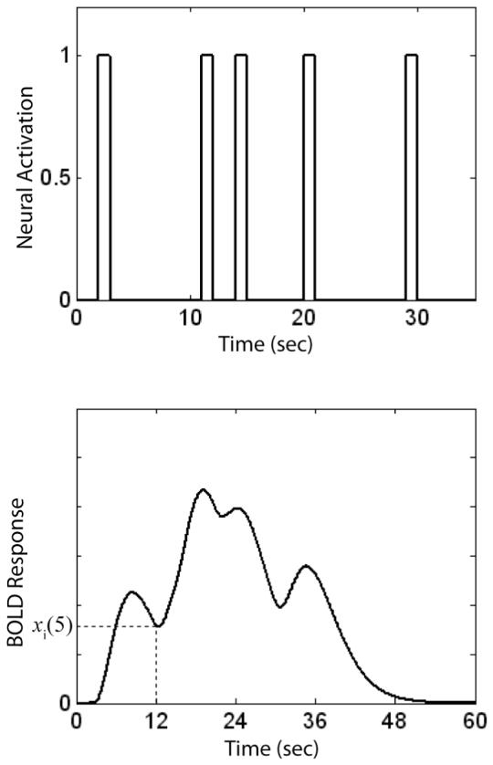
The top panel shows activation predicted by the boxcar model during 30 seconds of an event-related fMRI experiment. The bottom panel shows the predicted BOLD response under these same conditions.

Finally, as before, at each ROI we build the GLM:

$$\left[\begin{array}{c}\hfill B_i\left(1\right)\hfill \\ \hfill B_i\left(2\right)\hfill \\ \hfill ⋮\hfill \\ \hfill B_i\left(N\right)\hfill \end{array}\right]=\left[\begin{array}{ccc}\hfill w\left(1\right)\hfill & \hfill 1\hfill & \hfill 1\hfill \\ \hfill w\left(2\right)\hfill & \hfill 1\hfill & \hfill 2\hfill \\ \hfill ⋮\hfill & \hfill ⋮\hfill & \hfill ⋮\hfill \\ \hfill w\left(N\right)\hfill & \hfill 1\hfill & \hfill N\hfill \end{array}\right]\left[\begin{array}{c}\hfill {\theta }_C\hfill \\ \hfill B_0\hfill \\ \hfill \Delta \hfill \end{array}\right]+\left[\begin{array}{c}\hfill {\epsilon }_1\hfill \\ \hfill {\epsilon }_2\hfill \\ \hfill ⋮\hfill \\ \hfill {\epsilon }_N\hfill \end{array}\right]$$ (11)

where θ_C measures the correlation between the predictions of the boxcar model and the data.

Step 4: Compare the Two Models

A strong test of our model is to ask whether it provides a better fit than the boxcar model. Both models are the same except for the first column of the design matrix X. A poor fit of a model will mean larger residuals at each TR and consequently, a larger estimate of the error variance ${\sigma }_{\epsilon }^2$. Therefore, the magnitude of the error variance can be used as a measure of goodness-of-fit. In fact, at each ROI the goodness-of-fit measure BIC for model i (i = our model, or comparison model) is equal to

$$\mathit{BIC}\left(\text{Model}\mathrm{i}\right)=(N-3)\ln {\widehat{\sigma }}_i^2+3\ln (N-3).$$ (12)

Since N is the same for the two models, the model with the smaller error variance will have the smaller BIC, and when comparing BIC scores for various models the model with the smallest BIC score is chosen as the best. Therefore, we can conclude that our model gives a better account of the data than the boxcar model if its BIC score is lower in each ROI. Note that such a result is more impressive than it might first seem, because our model specifies the ROIs a priori. In contrast, the boxcar model makes no predictions about which brain regions should show task-related activation. In fact, in traditional exploratory fMRI data analyses, this boxcar model is applied to the data from every voxel in the brain and those voxels for which the null hypothesis

$${\mathrm{H}}_0:{\theta }_C=0$$

is rejected are classified as task-sensitive.

Although there is no statistical test to determine whether the BIC score of one model is significantly better than the BIC score of another model, quantitative conclusions can nevertheless be drawn. One possibility is to use the difference in BIC scores to compute the Bayes factor, which estimates the probability that the better fitting model is the correct model of the two (e.g., Raftery, 1995). For example, the approximate probability that our model is correct, assuming that either our model or the boxcar model is correct equals

$$\mathrm{P}(\text{our model is correct}\mid \text{Data})\doteq \frac{1}{1+\exp \{-\frac{1}{2}[\mathrm{BIC}\left(\text{our model}\right)-\mathrm{BIC}\left(\text{boxcar model}\right)]\}}.$$

Thus, for example, if our model fits better by a BIC difference of 2, then the probability that our model is correct is approximately .73, whereas if the BIC difference is 10, then this probability is approximately .99.

QUALITATIVE TESTS

Another way to avoid problems caused by inaccurate models of the hrf is to test predictions of the model in a more qualitative fashion. One attractive possibility in this domain is to compute the coherence between the predictions of the model and the observed BOLD response in each ROI (Sun, Miller, & D’Esposito, 2004). Coherence is a measure of correlation, but in the frequency domain, rather than the time domain. Whereas the standard Pearson correlation would be reduced if an inaccurate hrf was used to generate the model’s predictions, the coherence would be unaffected. If superposition holds, then the coherence between two BOLD responses equals the coherence between the neural activations that elicited those BOLD responses. In addition, coherence at low frequencies is unaffected by the presence of (high frequency) independent noise. Thus, coherence analysis avoids some of the most significant problems that plague standard correlational techniques.

Coherence analysis can also be used to test quantitative predictions of our model about the temporal delay between the onset of neural activations in two brain regions. This analysis uses the phase spectrum of the cross-correlation function between the BOLD responses from the two regions. Assuming that certain conditions are met, the temporal delay between the onset of the neural activations in the two regions is proportional to the slope of this phase spectrum (Sun, Miller, & D’Esposito, 2005).

Qualitative predictions about causality can also be tested by computing the Granger causality between BOLD responses in pairs of ROIs. For example, if a model predicts that activation in region A causes activation in region B, the observed BOLD responses from regions A and B can be used in a Granger causality analysis to test this prediction statistically (Geweke, 1982).

CONCLUSIONS

Functional MRI has revolutionized Psychology, but to date, almost all applications have been exploratory in nature. We believe that fMRI has tremendous untapped potential to provide rigorous and unique tests of computational models. As just one example, many computational models of working memory assign a key role to the head of the caudate nucleus. However, these models disagree as to whether the primary role of the caudate during working memory tasks is to provide a phasic, gating input to thalamus (i.e., via the globus pallidus) (e.g., Beiser & Houk, 1998; Frank, Loughry, & O’Reilly, 2001) or a tonic, sustained input (e.g., Ashby et al., 2005; Monchi et al., 2000). Testing between these alternatives with behavioral or lesion data would be extremely difficult, but the fMRI predictions of these two classes of models are quite different. As a result, we believe the techniques proposed in this article could be used to resolve this debate.

Some new problems must be solved when fMRI is used in this confirmatory manner, but for the most part, the statistical methods required are straightforward extensions of currently popular techniques. It is important to acknowledge that other solutions are possible. However, since there is currently no accepted method for fitting models to fMRI data, we believe that the methods described in this article represent a reasonable first solution. Most importantly, we hope that this article encourages researchers to expand their use of fMRI into the confirmatory domain.

REFERENCES

- Anderson JR, Qin Y. Using brain imaging to extract the structure of complex events at the rational time band. Journal of Cognitive Neuroscience. doi: 10.1162/jocn.2008.20108. in press. [DOI] [PMC free article] [PubMed] [Google Scholar]
- Ashby FG, Ell SW, Valentin VV, Casale MB. FROST: A distributed neurocomputational model of working memory maintenance. Journal of Cognitive Neuroscience. 2005;17:1728–1743. doi: 10.1162/089892905774589271. [DOI] [PubMed] [Google Scholar]
- Ashby FG, Ennis JM, Spiering BJ. A neurobiological theory of automaticity in perceptual categorization. Psychological Review. 2007;114:632–656. doi: 10.1037/0033-295X.114.3.632. [DOI] [PubMed] [Google Scholar]
- Beiser DG, Houk JC. Model of cortical-basal ganglionic processing: Encoding the serial order of sensory events. Journal of Neurophysiology. 1998;79:3168–3188. doi: 10.1152/jn.1998.79.6.3168. [DOI] [PubMed] [Google Scholar]
- Boynton GM, Engel SA, Glover GH, Heeger DJ. Linear systems analysis of functional magnetic resonance imaging in human V1. Journal of Neuroscience. 1996;16:4207–4221. doi: 10.1523/JNEUROSCI.16-13-04207.1996. [DOI] [PMC free article] [PubMed] [Google Scholar]
- Brown JW, Braver TS. Learned predictions of error likelihood in the anterior cingulate cortex. Science. 2005;307:1118–1121. doi: 10.1126/science.1105783. [DOI] [PubMed] [Google Scholar]
- Buxton RB, Wong EC, Frank LR. Dynamics of blood flow and oxygenation changes during brain activation: the balloon model. Magnetic Resonance in Medicine. 1998;39:855–864. doi: 10.1002/mrm.1910390602. [DOI] [PubMed] [Google Scholar]
- Chadderdon G, Sporns O. A large-scale neurocomputational model of task-oriented behavior selection and working memory in prefrontal cortex. Journal of Cognitive Neuroscience. 2006;18:242–257. doi: 10.1162/089892906775783624. [DOI] [PubMed] [Google Scholar]
- Chen CT. Introduction to linear systems theory. Holt, Rinehart and Winston; New York: 1970. [Google Scholar]
- Clark VP, Maisog JM, Haxby JV. fMRI studies of face memory using random stimulus sequences. Journal of Neurophysiology. 1998;79:3257–3265. doi: 10.1152/jn.1998.79.6.3257. [DOI] [PubMed] [Google Scholar]
- Cohen MS. Parametric analysis of fMRI data using linear systems methods. NeuroImage. 1997;6:93–103. doi: 10.1006/nimg.1997.0278. [DOI] [PubMed] [Google Scholar]
- Dale AM, Buckner RL. Selective averaging of rapidly presented individual trials using fMRI. Human Brain Mapping. 1997;5:329–340. doi: 10.1002/(SICI)1097-0193(1997)5:5<329::AID-HBM1>3.0.CO;2-5. [DOI] [PubMed] [Google Scholar]
- Danker JF, Anderson JR. The roles of prefrontal and posterior parietal cortex in algebra problem solving: A case of using cognitive modeling to inform neuroimaging data. NeuroImage. 2007;35:1365–1377. doi: 10.1016/j.neuroimage.2007.01.032. [DOI] [PubMed] [Google Scholar]
- Frank MJ, Claus ED. Anatomy of a decision: Striato-orbitofrontal interactions in reinforcement learning, decision making and reversal. Psychological Review. 2006;113:300–326. doi: 10.1037/0033-295X.113.2.300. [DOI] [PubMed] [Google Scholar]
- Frank MJ, Loughry B, O’Reilly RC. Interactions between frontal cortex and basal ganglia in working memory: A computational model. Cognitive, Affective, and Behavioral Neuroscience. 2001;1:137–160. doi: 10.3758/cabn.1.2.137. [DOI] [PubMed] [Google Scholar]
- Fransson P, Kruger G, Merboldt KD, Frahm J. MRI of functional deactivation: Temporal and spatial characteristics of oxygenation-sensitive responses in human visual cortex. NeuroImage. 1999;9:611–618. doi: 10.1006/nimg.1999.0438. [DOI] [PubMed] [Google Scholar]
- Friston KJ, Holmes AP, Ashburner J. Statistical Parametric Mapping (SPM) 1999 http://www.fil.ion.ucl.ac.uk/spm/
- Friston KJ, Josephs O, Ress G, Turner R. Nonlinear event-related responses in fMRI. Magnetic Resonance in Medicine. 1998;39:41–52. doi: 10.1002/mrm.1910390109. [DOI] [PubMed] [Google Scholar]
- Geweke J. Measurement of linear dependence and feedback between multiple time series. Journal of the American Statistical Association. 1982;77:304–313. [Google Scholar]
- Glover GH. Deconvolution of impulse response in event-related BOLD fMRI. NeuroImage. 1999;9:416–429. doi: 10.1006/nimg.1998.0419. [DOI] [PubMed] [Google Scholar]
- Henson R, Friston K. Convolution models for fMRI. In: Friston KJ, Ashburner JT, Kiebel SJ, Nichols TE, Penny WD, editors. Statistical parametric mapping: The analysis of functional brain images. Academic Press; London: 2007. pp. 178–192. [Google Scholar]
- Hinrichs H, Scholz M, Tempelmann C, Woldorff MG, Dale AM, Heinze HJ. Deconvolution of event-related fMRI responses in fast-rate experimental designs: Tracking amplitude variations. Journal of Cognitive Neuroscience. 2000;12:76–89. doi: 10.1162/089892900564082. [DOI] [PubMed] [Google Scholar]
- Huettel SA, McCarthy G. Evidence for a refractory period in the hemodynamic response to visual stimuli as measured by MRI. Neuroimage. 2000;11:547–553. doi: 10.1006/nimg.2000.0553. [DOI] [PubMed] [Google Scholar]
- Mason RA, Just MA. Neuroimaging contributions to the understanding of discourse processes. In: Traxler M, Gernsbacher MA, editors. Handbook of Psycholinguistics. Elsevier; Amsterdam: 2006. pp. 765–799. [Google Scholar]
- Monchi O, Taylor JG, Dagher A. A neural model of working memory processes in normal subjects, Parkinson’s disease, and schizophrenia for fMRI design and predictions. Neural Networks. 2000;13:953–973. doi: 10.1016/s0893-6080(00)00058-7. [DOI] [PubMed] [Google Scholar]
- Ogawa S, Lee TM, Kay AR, Tank DW. Brain magnetic resonance imaging with contrast dependent on blood oxygenation. Proceedings of the National Academy of Sciences. 1990;87:9868–9872. doi: 10.1073/pnas.87.24.9868. [DOI] [PMC free article] [PubMed] [Google Scholar]
- Ogawa S, Lee TM, Stepnoski R, Chen W, Zhu XH, Ugurbil K. An approach to probe some neural systems interaction by functional MRI at neural time scale down to milliseconds. Proceeding of the National Academy of Sciences USA. 2000;97:11026–11031. doi: 10.1073/pnas.97.20.11026. [DOI] [PMC free article] [PubMed] [Google Scholar]
- Ollinger JM, Shulman GL, Corbetta M. Separating processes within a trial in event-related functional MRI. I. The method. NeuroImage. 2001a;13:210–217. doi: 10.1006/nimg.2000.0710. [DOI] [PubMed] [Google Scholar]
- Ollinger JM, Shulman GL, Corbetta M. Separating processes within a trial in event-related functional MRI. II. Analysis. NeuroImage. 2001b;13:218–229. doi: 10.1006/nimg.2000.0711. [DOI] [PubMed] [Google Scholar]
- O’Reilly RC. Biologically based computational models of high-level cognition. Science. 2006;314:91–94. doi: 10.1126/science.1127242. [DOI] [PubMed] [Google Scholar]
- Pfeuffer J, McCullough JC, Van de Moortele P-F, Ugurbil K, Hu X. Spatial dependence of the nonlinear BOLD response at short stimulus duration. NeuroImage. 2003;18:990–1000. doi: 10.1016/s1053-8119(03)00035-1. [DOI] [PubMed] [Google Scholar]
- Raftery AE. Bayesian model selection in social research. Sociological Methodology. 1995;25:111–163. [Google Scholar]
- Sun FT, Miller LM, D’Esposito M. Measuring interregional functional connectivity using coherence and partial coherence analyses of fMRI data. NeuroImage. 2004;21:647–658. doi: 10.1016/j.neuroimage.2003.09.056. [DOI] [PubMed] [Google Scholar]
- Sun FT, Miller LM, D’Esposito M. Measuring temporal dynamics of functional networks using phase spectrum of fMRI data. NeuroImage. 2005;28:227–237. doi: 10.1016/j.neuroimage.2005.05.043. [DOI] [PubMed] [Google Scholar]
- Vazquez AL, Noll DC. Non-linear aspects of the blood oxygenation response in functional MRI. NeuroImage. 1998;8:108–118. doi: 10.1006/nimg.1997.0316. [DOI] [PubMed] [Google Scholar]
- Zarahn E, Aquirre G, D’Esposito M. A trial-based experimental design for fMRI. NeuroImage. 1997;6:122–138. doi: 10.1006/nimg.1997.0279. [DOI] [PubMed] [Google Scholar]