Abstract
Taxonomic inventories (or species censuses) are the most elementary data in biogeography, macroecology and conservation biology. They play fundamental roles in the construction of species richness patterns, delineation of species ranges, quantification of extinction risk and prioritization of conservation efforts in hot spot areas. Given their importance, any issue related to the completeness of taxonomic inventories can have far-reaching consequences. Here, we used the largest publicly available database of georeferenced marine fish records to determine its usefulness in depicting the diversity and distribution of this taxonomic group. All records were grouped at multiple spatial resolutions to generate accumulation curves, from which the expected number of species were extrapolated using a variety of nonlinear models. Comparison of the inventoried number of species with that expected from the models was used to calculate the completeness of the taxonomic inventory at each resolution. In terms of the global number of fish species, we found that approximately 21% of the species remain to be described. In terms of spatial distribution, we found that the completeness of taxonomic data was highly scale dependent, with completeness being lower at finer spatial resolutions. At a 3° (approx. 350 km2) spatial resolution, less than 1.8% of the world's oceans have above 80% of their fish fauna currently described. Censuses of species were particularly incomplete in tropical areas and across the entire range of countries' gross domestic product (GDP), although the few censuses nearing completion were all along the coasts of a few developed countries or territories. Our findings highlight that failure to quantify the completeness of taxonomic inventories can introduce substantial flaws in the description of diversity patterns, and raise concerns over the effectiveness of conservation strategies based upon data that remain largely precarious.
Keywords: taxonomic census, fishes, completeness, global, spatial scales, species
1. Introduction
The report of species at specific sites is probably the most basic data in ecology (Gaston & Blackburn 2000). Such records are often used to calculate the number of species occurring at each site or as a source of information with which to extrapolate the extent of species' occurrence and their area of occupancy (Gaston & Blackburn 2000). Further uses of these data vary from the construction of diversity patterns (Roy et al. 1998; Myers et al. 2000; Bellwood & Hughes 2001; Macpherson 2002; Roberts et al. 2002; Mora et al. 2003; Mora & Robertson 2005; Worm et al. 2005; Grenyer et al. 2006) to the identification of ‘hot spots’ of extinction-prone species (Myers et al. 2000; Roberts et al. 2002) and to the creation of optimum conservation strategies (Myers et al. 2000; Roberts et al. 2002; Grenyer et al. 2006). Escalating anthropogenic impacts on biodiversity and the need to prioritize limited conservation resources have prompted the description of and attempts to understand diversity patterns and, therefore, have stimulated the use of taxonomic inventories (Roy et al. 1998; Myers et al. 2000; Bellwood & Hughes 2001; Macpherson 2002; Roberts et al. 2002; Mora et al. 2003; Mora & Robertson 2005; Worm et al. 2005; Grenyer et al. 2006). Determining the extent to which human-related threats affect biodiversity, either through the loss of species at given sites or through changes in range size, also requires accurate data on the distribution of species (Gaston & Blackburn 2000). A limitation with regard to the use of taxonomic inventories for these purposes is the extent of their completeness (i.e. the fraction of species in a given location that has been sampled). If some locations are more completely sampled than others, or if a species has not been reported in a given location due to insufficient sampling effort, this will introduce biases to the yielded patterns and to the subsequent analyses of ecological mechanisms and conservation strategies (Soberon & Llorente 1993; Colwell & Coddington 1994; Gotelli & Colwell 2001; Soberon et al. 2007). In this study, we used the largest publicly available database of georeferenced marine fish records to determine its usefulness in depicting the diversity and distribution of this taxonomic group. All records were grouped at multiple spatial resolutions to generate accumulation curves from which the expected number of species was extrapolated using a variety of nonlinear models (see Soberon et al. (2007) for a similar analysis with butterflies from Mexico). The results of the different models were averaged using a weighting approach based on an information-theoretic methodology. Comparison of the actual number of species with that expected from the models was used to calculate the completeness of the taxonomic inventory at each spatial resolution.
2. Material and methods
(a) Database
We used approximately 2.1 million records available for marine fishes in the Ocean Biogeographical Information System (OBIS). This database is part of the Census of Marine Life programme (extended details of the database can be found at www.iobis.org). Data included in the OBIS date back to the beginning of the modern Linnaean classification system 250 years ago, and consist of dated and georeferenced records of individual species but not their abundances. All data in the OBIS have been cross-checked with the Catalogue of Fishes to ensure that each record is valid based upon the most up-to-date taxonomy. The OBIS has been in operation since 1998 and has gathered data from all major public sources of marine biogeographical data such as the Global Biodiversity Information Facility, FishBase and Catalogue of Fishes, which have been themselves gathering data from numerous sources for a number of years. The OBIS also has a policy of easy data posting, which allows parties such as natural museums, regional organizations, scientific projects and individuals to post their data, and significant efforts have been made to encourage the posting of and free access to data (Grassle 2000; Costello & Vanden 2006). The accessibility of such data is critical to the global description and verification of diversity patterns; data that have been collected but not made publicly available cannot be used for these purposes. In the light of the fact that there are such inaccessible data, our results have to be interpreted as a synopsis of the combined state of public knowledge on the global distribution and diversity of marine fishes.
(b) Accumulation curves
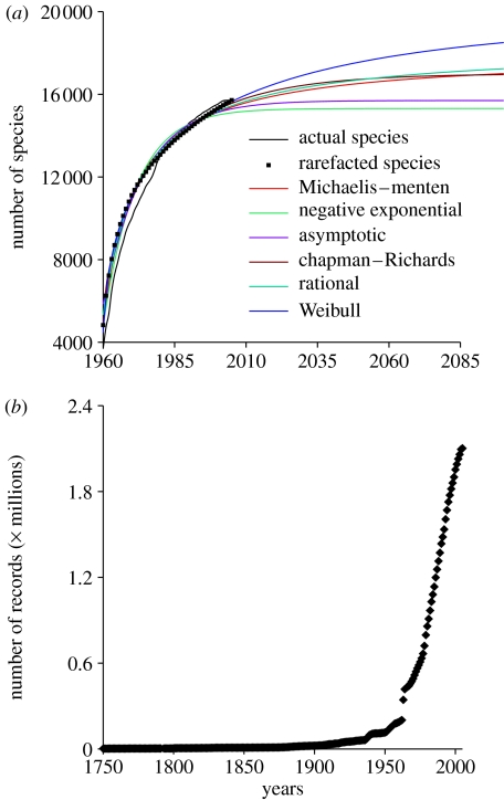
We calculated the completeness of taxonomic inventories within square cells across a range of spatial resolutions from 3° to 36° within the world's oceans and within the high seas and exclusive economic zones (EEZs) of the world. Using geographical information system software, records were assigned to a given cell, high sea or EEZ based on their geographical positions. We used the year of collection for each record to construct an accumulation curve of species over time within each of our spatial units. This temporal accumulation curve may be viewed as analogous to a ‘rate of discovery’ curve (May 1990), since each species only contributes to the curve upon first being reported within each spatial unit, despite any subsequent appearance in a sample. Data collected prior to 1960 were markedly patchy, due to the events such as the two world wars and perhaps varying taxonomic interest (Zapata & Robertson 2007; see also figure 2b). Therefore, data collected prior to that year were added to the models as a y-intercept. As recommended by other studies (Colwell & Coddington 1994; Gotelli & Colwell 2001), we used sample-based rarefaction to reduce biases introduced by inconsistencies and discontinuities in taxonomic effort. Each iteration of this Monte Carlo approach randomly ordered the years of the records to create an accumulation curve (this is equivalent to obtaining a number of species in a sample of n years). We repeated this approach 50 times for the data in each cell, high sea or EEZ, and averaged the resulting curves to get a smoothed species accumulation curve (a detailed description of this approach can be found in Colwell & Coddington (1994) and Gotelli & Colwell (2001)).
Figure 2.
Temporal description of marine fish species worldwide. (a) The species accumulation curve, the smoothed rarefaction curve and the fit of the nonlinear models to the global data. Results for the different models are shown in table 2. (b) The accumulation of records with date stamps in OBIS.
(c) Calculation of completeness
A number of parametric and non-parametric models have been put forward to estimate species richness through the extrapolation of discovery record data. However, comparative studies have indicated that the results of such models may vary considerably depending upon different attributes of the data (e.g. Colwell & Coddington 1994; Walther & Morand 1998; Gotelli & Colwell 2001; Shackell & Frank 2001; Cam et al. 2002; Foggo et al. 2003), and not surprisingly the models recommended by different studies usually vary. To overcome the problem of model selection, we used a model averaging approach (Burnham & Anderson 2002; Johnson & Omland 2003) to combine the results of different nonlinear models. This approach allows us to weight the models based on the support of the data, and to incorporate model selection uncertainty into confidence limits. The use of multimodel averaging has been argued to be statistically more accurate than the simplistic use of a unique model (e.g. Burnham & Anderson 2002). It should be noted that multimodel averaging uses fit estimators, and therefore it is suitable only for parametric models.
To calculate the total number of species occurring at any spatial resolution, we calculated the asymptotes of six nonlinear models fitted to the smoothed rarefaction curves (figure 2a; table 2). We used the bias-corrected form of Akaike's information criterion (AIC) to assess model performance (Burnham & Anderson 2002; Johnson & Omland 2003). AIC penalizes the addition of unnecessary parameters, and thus selects for a model that has the best combination of good fit and minimal number of parameters (i.e. simplicity, parsimony). We used multimodel averaging based on the AIC weight of each model to compute the asymptotic number of species expected. Per cent completeness at each spatial resolution was calculated by dividing the total number of species currently reported within the cell, high sea or EEZ by the averaged asymptotic value. We used the multimodel weighted average unconditional standard errors to calculate 95% CIs. The entire approach, from sorting the data, to running the simulations, to fitting the models, and to calculating completeness, was performed using a macro developed in Microsoft Excel. The models were fitted using DataFitX v. 2.0. by Oakdale Engineering. The results of this program were identical to those of a more popular statistical package such as Statistica. The former was preferred because it can be run directly from Excel allowing full automation of the procedure.
Table 2.
Results of the asymptotic nonlinear models fitted to the accumulation curve based on available records for all marine fish species of the world.
| model name | function | asymptote | 95% CI | AIC |
|---|---|---|---|---|
| Michaelis–Menten | Y=(a*x)/(1+(b*x)) | 17 957 | 17 685–18 229 | 488.4 |
| negative exponential | Y=a*(1−exp((−b)*x)) | 15 312 | 15 046–15 577 | 551 |
| asymptotic | Y=a−(b*(c^x)) | 15 699 | 15 414–15 985 | 525.3 |
| Chapman–Richards | Y=a*((1−exp(−b*x))^c) | 16 999 | 16 634–17 363 | 434 |
| rational | Y=(a+(b*x))/(1+(c*x)) | 18 325 | 18 025–18 639 | 474 |
| Weibull | Y=a*(1−exp(−(b*(x−c))^d)) | 19 800 | 19 082–20 518 | 358 |
(d) Assessment of biases
We defined as biases factors likely to consistently affect the accuracy (i.e. extent to which the predicted value approached the true value) with which our approach (see calculation of completeness above) predicted the true number of species at any given spatial unit. We assessed three factors that we believe may affect accuracy. Firstly, the natural variation in the number of individuals per species in natural communities (i.e. the relative species abundance frequency distribution, RSA). This affects the likelihood of sampling a given species per unit of sampling effort, which is known to affect the shape of the rarefaction curve (Gotelli & Graves 1994). Sampling a community with a more even distribution of individuals among species will detect species more quickly than a community with a long tail of rare species, and hence the rarefaction curve will rise more quickly to an asymptote (Gotelli & Graves 1994). Secondly, we assessed the effects of the temporal variation in sampling effort (figure 2b). Thirdly, the effect of using a variable number of sampled years in a curve. To assess these potential sources of bias, we created hypothetical communities, then simulated these factors and assessed the extent to which they affect the accuracy of our approach in predicting the true number of species.
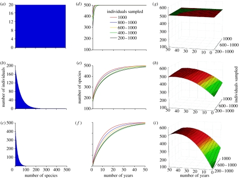
We simulated three hypothetical communities all with 10 000 individuals and 500 species but with different RSAs. The skews of the different RSAs were determined using a geometric series (GS) distribution, with the distribution of individuals among species being even (GS ratio=1.0001), uneven (GS ratio=1.02) and very uneven (GS ratio=1.05), (figure 1a–c). From each of these communities, we surveyed a random number of individuals per time (analogous to 1 ‘year’ of sampling) with an effort ranging from being highly variable to being always consistent (i.e. each time we surveyed between 200 and 1000 individuals, 400 and 1000, 600 and 1000, 800 and 1000 and always 1000). This simulates variable sampling effort that may exist in our database. Using these surveyed individuals, we created five sets of smoothed rarefaction curves (using the Monte Carlo approach described above), each of which used 10, 20, 30, 40 and 50 years of sampling (this simulates the variable number of sampled years that exist in the different analysed spatial units). Therefore, in summary, for each of our three hypothetical communities, we created 25 smoothed rarefaction curves combining variable sampling effort (for any given year) and variable number of years. To each of these curves, we fitted all nonlinear models and calculated the asymptotic maximum number of species in the subject community. This entire approach was repeated 50 times. The mean predicted number of species in the 50 iterations were compared graphically to assess variations in accuracy due to the different factors.
Figure 1.
(a–c) Effects of the RSA distribution and (d–f) variable sampling on the rarefaction curves and (g–i) on the asymptotic number of species predicted by the models. Here, we created three hypothetical communities each with 500 species and 10 000 individuals. (a–c) The number of individuals per species in each community ranged from being equal to very unequal, to generate RSAs with different skews. For each of these communities, we created rarefaction curves (d–f) by sampling a variable number of individuals for each time period (simulating the sampling occurred at any given year). Sampling effort varied by a factor of five: from 200 to 1000 individuals each time period, from 400 to 1000, from 600 to 1000, from 800 to 1000 and exactly 1000 individuals each time. We also created another set of curves (not shown) using 10, 20, 30, 40 and 50 years of sampling. Thus, for each community, we created a total of 25 curves, combining all five sampling efforts and five groups of years. For each of these of curves, we fitted all nonlinear models and applied the approach mentioned in §2 to calculate the predicted asymptotic number of species in the community (g–i).
3. Results and discussion
In assessing the effect of potential biases, we found that our approach tended to underpredict the true number of species among the two communities with some degree of skew in their RSA, and whose curves were based on less than 30 years of sampling (figure 1h,i). In those cases, accuracy decreased with reductions in the number of years included in a curve and with increases in the level of skew of the RSA. Exceptionally, our approach predicted the true number of species with an accuracy of 80% when a minimum of 10 years were included in a curve (figure 1h,i). Although we cannot use the OBIS data to predict the RSA of each community, examining the empirical data show that approximately 54% of the 3°×3° cells have less than 10 years of sampling, 30.6% of the 9°×9° cells, 19% of the 18°×18° cells and 8% of the 36°×36° cells. These results indicate that a higher level of caution should be applied to the results at smaller spatial scales, as these are likely to underestimate the true number of species to a greater degree. However, in those cases, our results will overestimate the true completeness of taxonomic inventories, or in other words, the taxonomic inventories may be more incomplete than what this study shows.
Based on the OBIS data, we found that at the global scale there are currently 15 716 marine fish species publicly described (figure 2a; table 1). We found that such a global census is approximately 79% complete or that approximately 4084 marine fish species remain to be described (figure 2a; table 1). The proportion of species remaining to be described is greater in the open and deep ocean (i.e. bathypelagic, bathydemersal and demersal habitats) and smaller in shallower and coastal areas (i.e. reef and benthopelagic habitats; table 1). These variations in the completeness of inventories among habitats probably reflect variations in the accessibility and facilities available to sample those habitats. For instance, the bathydemersal region, one of the most inaccessible and deepest marine environments, has the lowest census completeness. In contrast, shallower reef habitats are the most complete of all inventoried habitats (table 1). Pelagic fish species have also been well inventoried (table 1), which has previously been attributed to the large body size of most species in this environment and their ease of capture (Zapata & Robertson 2007).
Table 1.
Present-day completeness of the global taxonomic inventory of marine fishes by habitat and as a whole.
| habitat | currently described | asymptotic value | 95% CI | per cent completeness | species remaining |
|---|---|---|---|---|---|
| bathydemersal | 2081 | 3719 | 3594–3843 | 56 | 1638 |
| bathypelagic | 1275 | 1670 | 1591–1749 | 76 | 395 |
| benthopelagic | 908 | 1126 | 1105–1146 | 81 | 218 |
| demersal | 6159 | 8462 | 8039–8886 | 73 | 2303 |
| pelagic | 1052 | 1216 | 1192–1240 | 87 | 164 |
| reef associated | 4241 | 4611 | 4543–4679 | 92 | 370 |
| all species | 15 716 | 19 800 | 19 082–20 518 | 79 | 4084 |
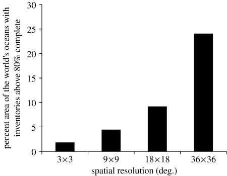
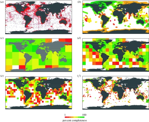
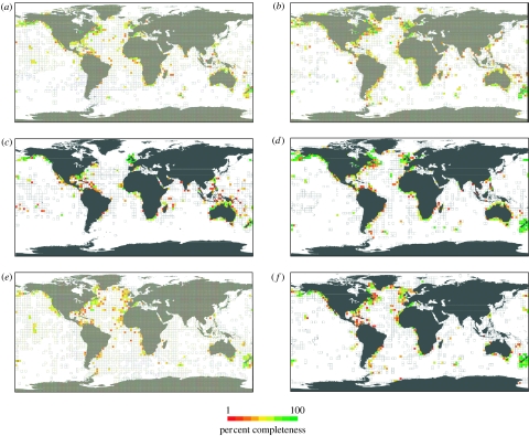
We found that the completeness of taxonomic censuses is highly scale dependent, being particularly low at finer spatial resolutions (figure 3). At a relatively broad 36° resolution, 24% of the world's oceans area has inventories above 80% complete (figures 3 and 4c). In contrast, at a finer 3° resolution, only 1.8% of the world's oceans have inventories above that level of completeness (figures 3 and 4f). These findings highlight a significant issue in current marine biogeographical and conservation research. Firstly, large-scale diversity patterns are built upon species data recorded at finer resolutions (Levin 1992; Roy et al. 1998; Bellwood & Hughes 2001; Macpherson 2002; Mora et al. 2003; Mora & Robertson 2005; Worm et al. 2005). Unfortunately, the few relatively complete inventories are not continuously distributed in space so as to warrant reliable patterns, even at regional scales (figure 4f). Moreover, there was a very poor congruence between current and expected numbers of species, suggesting that patterns based on existing data may not be a good surrogate for true diversity patterns (with the exception of the coarse resolution (i.e. 36° cells), R2 between observed and expected species was smaller than 0.001; figure 4). A problem that may arise due to unreliable diversity patterns is the accuracy of tests about their causes or mechanisms. If existing diversity patterns fail to accurately depict true diversity, then support for inference of causal mechanisms from and for these patterns should be treated with caution. Finally, these results raise uncertainty on the effectiveness of conservation strategies aimed at protecting marine fish biodiversity. For conservation research, the issue is particularly critical because high-resolution data are commonly used as the basis from which to estimate species' extinction risk (Gaston & Blackburn 2000), and because some of the main threats to biodiversity often occur at small scales (Grenyer et al. 2006), and it is at those scales that decisions are made (Roy et al. 1998; Bellwood & Hughes 2001; Macpherson 2002; Mora et al. 2003; Mora & Robertson 2005; Worm et al. 2005; Grenyer et al. 2006) and where data are particularly precarious (figure 4f).
Figure 3.
Area of the world's oceans with taxonomic censuses over 80% complete at various spatial resolutions.
Figure 4.
Taxonomic sampling of the marine fishes of the world. (a) The positions of the approximately 2.1 million georeferenced records used in this study. (b) The completeness of the taxonomic inventories within the high seas and EEZs of the world. (c–f) Resolutions of 36°×36°, 18°×18°, 9°×9°, and 3°×3°, respectively. White areas in the maps indicate locations whose curves have less than 10 years sampled. Congruence between the number of species observed and expected was R2=0.0098, n=1318, p<0.3 (at 3°×3°); R2=0.00002, n=409, p<0.9 (at 9°×9°); R2=0.0001, n=151, p<0.87 (at 18°×18°); and R2=0.85, n=48, p<0.001 (at 36°×36°).
Incomplete taxonomic inventories were not distributed uniformly in space. Globally, most records for marine species have been collected near the vicinity of continental coasts and are concentrated within the EEZs of few countries (figure 4a). Consequently, existing records yield taxonomic inventories over 80% complete for the coasts of only a few developed countries or territories (Canada, Australia, Alaska, the United Kingdom, the United States, Greenland, Republic of South Africa and Bermuda). In general, however, incomplete inventories were common across the range of countries' wealth (completeness versus gross domestic product purchasing power parity (GDP PPP): R2=0.046, n=90 EEZs, p<0.05; completeness versus GDP PPP per capita: R2=0.08, n=90 EEZs, p<0.006). Forty-four countries have inventories between 50 and 80% complete, and 175 countries have inventories below 50% completion (figure 4b). All of the high seas have inventories below 50% completion. Remarkably, tropical areas that are well-known for their diversity have among the lowest completeness of all taxonomic inventories (figure 4c–f). These data gaps occurred regardless of habitat (figure 5; table 2).
Figure 5.
Completeness of taxonomic inventories by marine habitat. Completeness of taxonomic inventories was determined at a 3° resolution for species residing in different marine habitats. Species-specific habitat associations were obtained from Froese & Pauly (2006). They were as follows: (a) pelagic, (b) demersal, (c) reef associated, (d) benthopelagic, (e) bathypelagic and (f) bathydemersal (details of each of the habitats can be found in Froese & Pauly (2006)). For a spatial reference of where the different habitats may occur (i.e. all delimited cells), we selected all the cells where at least one species with a particular habitat association has been described.
Significant efforts have been made to improve and synthesize the taxonomy of marine fishes (e.g. Eschmeyer 1998) and to index information on their biology, distribution and diversity (e.g. Froese & Pauly 2006). However, our results indicate that these enormous efforts fall short for describing the worldwide diversity and distribution of marine fishes with reasonable accuracy, particularly at smaller spatial scales. Fishes are one of the most intensively studied marine taxonomic groups, suggesting that the situation may well be worse among other marine taxa. This scarcity of data occurs nearly 250 years since species first started to be described according to the Linnaean system of classification. Given that current projections on biodiversity change and the extent of human threats predict major biodiversity losses within the next half of a century (Thomas et al. 2004; Worm et al. 2006), many species may be lost without us ever knowing they existed. The precarious nature of existing data also highlights potential flaws in the accuracy of existing patterns. Our spurious knowledge about the current distribution of marine fish species also raises concern upon the effectiveness of existing conservation efforts aimed at protecting biodiversity and upon the future quantification of human-driven extinctions. With biodiversity increasingly being threatened by human-related activities, the uncertainty arising from incomplete data is a problem needing to be rapidly addressed. Though remarkable effort and progress have been made, a solution to this data gap is going to require considerable renewed interest in taxonomy by both researchers and funding agencies, and a continuation of effort among researchers and publishing journals to encourage the storage of raw data in publicly available databases.
Acknowledgments
We extend our thanks to the Ocean Biogeographic Information System and all contributing databases and scientists for making their data freely available. Phoebe Zhang collaborated with the organization and transfer of data. Funding was provided by the Sloan Foundation Census of Marine Life through the Future of Marine Animal Populations (FMAP) programme. We thank Peter Sale, Frederick Grassle, Walter Jetz, Heike Lotze, Boris Worm and Kevin Gaston for their helpful comments.
References
- Bellwood D.R, Hughes T. Regional-assembly rules and biodiversity of coral reefs. Science. 2001;292:1532–1535. doi: 10.1126/science.1058635. doi:10.1126/science.1058635 [DOI] [PubMed] [Google Scholar]
- Burnham K.P, Anderson D.R. Springer; New York, NY: 2002. Model selection and multi-model inference: a practical information-theoretic approach. [Google Scholar]
- Cam E, Nichols J.D, Sauer J.R, Hines J.E. On the estimation of species richness based on the accumulation of previously unrecorded species. Ecography. 2002;25:102–108. doi:10.1034/j.1600-0587.2002.250112.x [Google Scholar]
- Colwell R.K, Coddington J.A. Estimating terrestrial biodiversity through extrapolation. Phil. Trans. R. Soc. B. 1994;345:101–118. doi: 10.1098/rstb.1994.0091. doi:10.1098/rstb.1994.0091 [DOI] [PubMed] [Google Scholar]
- Costello M, Vanden E. ‘Ocean biodiversity informatics’: a new era in marine biology research and management. Mar. Ecol. Prog. Ser. 2006;316:203–214. doi:10.3354/meps316203 [Google Scholar]
- Eschmeyer W.N. California Academy of Sciences Press; San Francisco, CA: 1998. The catalog of fishes. [Google Scholar]
- Foggo A, Attrill M.J, Frost M.T, Rowden A.A. Estimating marine species richness: an evaluation of six extrapolative techniques. Mar. Ecol. Prog. Ser. 2003;248:15–26. doi:10.3354/meps248015 [Google Scholar]
- Froese, R. & Pauly, D. 2006. FishBase See www.fishbase.org
- Gaston K.J, Blackburn T.M. Blackwell Science; Oxford, UK: 2000. Pattern and process in macroecology. [Google Scholar]
- Gotelli N.J, Colwell R.K. Quantifying biodiversity: procedures and pitfalls in the measurement and comparison of species richness. Ecol. Lett. 2001;4:379–391. doi:10.1046/j.1461-0248.2001.00230.x [Google Scholar]
- Gotelli N.J, Graves G.R. Smithsonian Institution Press; Washington, DC: 1994. Null models in ecology. [Google Scholar]
- Grassle J.F. The Ocean Biogeographic Information System (OBIS): an on-line, worldwide atlas for accessing, modeling and mapping marine biological data in a multidimensional geographic context. Oceanography. 2000;13:5–7. [Google Scholar]
- Grenyer R, et al. Global distribution and conservation of rare and threatened vertebrates. Nature. 2006;444:93–96. doi: 10.1038/nature05237. doi:10.1038/nature05237 [DOI] [PubMed] [Google Scholar]
- Johnson J.B, Omland K.S. Model selection in ecology and evolution. Trends Ecol. Evol. 2003;19:101–108. doi: 10.1016/j.tree.2003.10.013. doi:10.1016/j.tree.2003.10.013 [DOI] [PubMed] [Google Scholar]
- Levin S.A. The problem of pattern and scales in ecology. Ecology. 1992;76:1943–1967. doi:10.2307/1941447 [Google Scholar]
- Macpherson E. Large-scale species richness gradients in the Atlantic Ocean. Proc. R. Soc. B. 2002;269:1715–1720. doi: 10.1098/rspb.2002.2091. doi:10.1098/rspb.2002.2091 [DOI] [PMC free article] [PubMed] [Google Scholar]
- May R.M. How many species? Phil. Trans. R. Soc. B. 1990;330:293–304. doi:10.1098/rstb.1990.0200 [Google Scholar]
- Mora C, Robertson D.R. Causes of latitudinal gradients in species richness: a test with the endemic shorefishes of the tropical eastern pacific. Ecology. 2005;86:1771–1782. doi:10.1890/04-0883 [Google Scholar]
- Mora C, Chittaro P.M, Sale P.F, Kritzer J, Ludsin S.A. Patterns and processes in reef fish diversity. Nature. 2003;421:933–936. doi: 10.1038/nature01393. doi:10.1038/nature01393 [DOI] [PubMed] [Google Scholar]
- Myers N, Mittermeier R.A, Mittermeier C.G, da Fonseca G, Kent J. Biodiversity hotspots for conservation priorities. Nature. 2000;403:853–858. doi: 10.1038/35002501. doi:10.1038/35002501 [DOI] [PubMed] [Google Scholar]
- Roberts C.M, et al. Marine biodiversity hotspots and conservation priorities for tropical reefs. Science. 2002;295:1280–1284. doi: 10.1126/science.1067728. doi:10.1126/science.1067728 [DOI] [PubMed] [Google Scholar]
- Roy K, Jablonski D, Valentine J.W, Rosenberg G. Marine latitudinal gradients: test of causal hypotheses. Proc. Natl Acad. Sci. USA. 1998;95:3699–3702. doi: 10.1073/pnas.95.7.3699. doi:10.1073/pnas.95.7.3699 [DOI] [PMC free article] [PubMed] [Google Scholar]
- Shackell N.L, Frank K.T. Marine fish diversity on the Scotian shelf, Canada. Aquat. Conserv. Mar. Freshw. Ecosyst. 2001;13:305–321. doi:10.1002/aqc.554 [Google Scholar]
- Soberon J, Llorente J. The use of accumulation functions for prediction of species richness. Conserv. Biol. 1993;7:480–488. doi:10.1046/j.1523-1739.1993.07030480.x [Google Scholar]
- Soberon J, Jimenez R, Golubov J, Koleff P. Assessing completeness of biodiversity databases at different spatial scales. Ecography. 2007;30:152–160. doi:10.1111/j.2006.0906-7590.04627.x [Google Scholar]
- Thomas C.D, et al. Extinction risk from climate change. Nature. 2004;427:145–148. doi: 10.1038/nature02121. doi:10.1038/nature02121 [DOI] [PubMed] [Google Scholar]
- Walther B.A, Morand S. Comparative performance of species richness estimation methods. Parasitology. 1998;116:395–405. doi: 10.1017/s0031182097002230. doi:10.1017/S0031182097002230 [DOI] [PubMed] [Google Scholar]
- Worm B, Sandow M, Oschlies A, Lotze H.K, Myers R. Global patterns of predators diversity in the open oceans. Science. 2005;309:1365–1369. doi: 10.1126/science.1113399. doi:10.1126/science.1113399 [DOI] [PubMed] [Google Scholar]
- Worm B, et al. Impacts of biodiversity loss on ocean ecosystem services. Science. 2006;314:787–790. doi: 10.1126/science.1132294. doi:10.1126/science.1132294 [DOI] [PubMed] [Google Scholar]
- Zapata F, Robertson D.R. How many species of shore fishes are there in the Tropical Eastern Pacific? J. Biogeogr. 2007;34:38–51. doi:10.1111/j.1365-2699.2006.01586.x [Google Scholar]


