Sparse source imaging in electroencephalography with accurate field modeling

Abstract

We have developed a new L1‐norm based generalized minimum norm estimate (GMNE) and have fully characterized the concept of sparseness regularization inherited in the proposed algorithm, which is termed as sparse source imaging (SSI). The new SSI algorithm corrects inaccurate source field modeling in previously reported L1‐norm GMNEs and proposes that sparseness a priori should only be applied to the regularization term, not to the data term in the formulation of the regularized inverse problem. A new solver to the newly developed SSI has been adopted and known as the second‐order cone programming. The new SSI is assessed by a series of simulations and then evaluated using somatosensory evoked potential (SEP) data with both scalp and subdural recordings in a human subject. The performance of SSI is compared with other L1‐norm GMNEs and L2‐norm GMNEs using three evaluation metrics, i.e., localization error, orientation error, and strength percentage. The present simulation results indicate that the new SSI has significantly improved performance in all evaluation metrics, especially in the metric of orientation error. L2‐norm GMNEs show large orientation errors because of the smooth regularization. The previously reported L1‐norm GMNEs show large orientation errors due to the inaccurate source field modeling. The SEP source imaging results indicate that SSI has the best accuracy in the prediction of subdural potential field as validated by direct subdural recordings. The new SSI algorithm is also applicable to MEG source imaging. Hum Brain Mapp 2008. © 2007 Wiley‐Liss, Inc.

INTRODUCTION

Electroencephalography (EEG) has excellent temporal resolution in the study of human brain activity, and the EEG data are frequently interpreted using source models because of the nonuniqueness of the so‐called inverse problem [Nunez and Srinivasan,2005]. The most basic source model is the equivalent current dipole (ECD) [He et al.,1987; Henderson et al.,1975; Sidman et al.,1978], which assumes that the EEG potentials are generated by one or a few focal currents. Each focal source can be modeled by an ECD with six parameters: three location parameters, two orientation parameters, and one moment (or strength) parameter [He et al.,1987]. The ECDs can be further classified as fixed dipoles, rotating dipoles, or moving dipoles with different freedoms in the parameter space, depending on how much prior knowledge is available for the investigated system. The parameter of importance for ECD is the number of current dipoles which is usually determined according to ad hoc assumptions. Given a specific ECD model, the dipole source localization can then be solved using least‐squares methods by minimizing the difference between the model‐predicted and the measured potentials.

Although the focal currents can be modeled using the ECDs, the distributed current sources are more popularly characterized by a distributed current density source model [Dale and Sereno,1993; Hämäläinen and Ilmoniemi,1984], which reconstructs current sources by finding the most probable current distribution that adequately explains the measured data [He and Lian,2005]. The source space is usually represented by distributed voxels, with small intervoxel distance, each of which stands for a local current source. The voxels normally cover the entire human brain within which the EEG signals are generated. Its inverse problem is fundamentally nonunique, in that there are an infinite number of source configurations that could explain a given measurement [He,1999]. An anatomical constraint has been introduced to constrain the possible source configuration on the cortical gray matter because empirical and theoretical evidence suggests that the majority of the observed scalp EEG signals arise from the cortical gray matter [Dale and Sereno,1993]. However, the highly convoluted human cortex (i.e., sulci and gyri) requires a high‐density voxel representation, and its inverse problem is, therefore, underdetermined and requires either explicit or implicit prior constraints on the allowed source fields to obtain a unique solution. This fact has led to the development of the minimum norm estimate (MNE) that selects the current distribution which explains the measured data with the smallest Euclidean norm (L2‐norm) [Hämäläinen and Ilmoniemi,1984], and its variants [Gorodnitsky et al.,1995; He et al.,2002a; Jeffs et al.,1987; Liu et al.,1998; Pascual‐Marqui et al.,1994]. The MNE algorithms produce low‐resolution solutions of cortical sources spreading over multiple cortical sulci and gyri, which do not reflect the generally sparse and compact nature of most cortical activations evidenced by functional magnetic resonance imaging (fMRI) data. In an attempt to produce more physiologically plausible images that can be obtained using the MNE, the generalized minimum norm estimate (GMNE) algorithms using the L1‐norm instead of the L2‐norm have been explored [Matsuura and Okabe,1995; Uutela et al.,1999; Wagner et al.,1998]. The attractiveness of these approaches is that they can be solved by a linear programming (LP) method, and the properties of LP guarantee that there exists an optimal solution for which the number of nonzero sources does not exceed the number of measurements and the solutions are therefore guaranteed to be sparse and compact. The advantage of these approaches has been investigated in both simulation studies [Silva et al.,2004; Yao and Dewald,2005] and experimental studies [Hann et al.,2000; Pulvermüller et al.,2003].

One problem arising in the currently available L1‐norm GMNEs is that their solutions have an orientation discrepancy which tends to align the dipole source at each voxel with the coordinate axes. Its mathematic explanation will be given later in the Method section. In the first attempt of L1‐norm GMNE [Matsuura and Okabe,1995], such discrepancy was simply ignored due to the fact that LP could not handle it. Wagner et al. [1998] proposed a new decomposition for a vector source in a coordinate system with 12 or even 20 axes to minimize the orientation discrepancy. The number of axes could theoretically be infinite. However, it is still an approximation and, only with an infinite number of axes, the orientation discrepancy will be diminished, which is computationally unrealistic. Uutela et al. [1999] developed a two‐step procedure, i.e., minimum current estimate (MCE). They implemented the L2‐norm GMNE in the first step to estimate source orientations, which were subsequently used to constrain the vector source field into a scalar field in the second step of the L1‐norm GMNE. The accuracy of the L1‐norm GMNE depends on the orientation accuracy estimated by the L2‐norm GMNE.

The aim of the present study is to develop a new sparse source imaging (SSI) technique by solving the orientation discrepancy problem. This task was achieved by second‐order cone programming (SOCP) instead of LP. In the noiseless case, we compared it with the previously reported L1‐norm GMNEs and the imaging error caused by the orientation discrepancy was demonstrated. In the noisy cases, Monte Carlo simulations were used in the comparison studies performed among the proposed SSI algorithm and other L1‐norm and L2‐norm GMNEs. After completing the simulation studies, we further evaluated their performance using scalp and subdural recorded somatosensory evoked potentials (SEPs) in a human subject. The independent measurements of the subdural SEPs provided a way for us to determine whether the solutions obtained with the various source imaging methods were reasonable or not.

METHODS

Sparse Source Imaging

For the distributed current density model, the linear relationship between the EEG recordings and the current sources at any voxel can be expressed as

(1)

where ϕ is the vector of instantaneous EEG recordings, A is the lead field, s is the current source vector, and n is the noise vector. Since the number of sources is larger than the number of measurements, the regularized formulation of the inverse problem can be derived from the Bayesian theory and stated as

(2)

where C(s) is the cost function, ‖ϕ − As‖²is the data term, f(s) is the source field model term, and λ is the regularization parameter. The source field model is known as regularization term which gives prior knowledge about the source field. In GMNEs, the norm of solution vector is used to describe the global strength of source field. The Euclidean norm, f(s) = ‖ s ‖${}_{\text{2}}^{\text{2}}$, is adopted in the L2‐norm GMNE, while f(s) = ‖ s ‖₁ is used in the L1‐norm GMNE. The priors in GMNEs with either the L2‐ or L1‐norm could be interpreted, from the Bayesian theory, as a probabilistic model that describes the expectations concerning the statistical properties of current source field [Baillet and Garnero,1997; Liu et al.,2002]. L2‐norm GMNEs use a Gaussian a priori current field as its probabilistic model which produces the smooth source imaging and, meanwhile, L1‐norm GMNEs adopt an exponential current field (Fig. 1c) that introduces the sparseness a priori into the problem and leads to the SSI.

Figure 1.

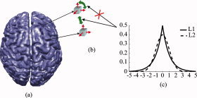
Illustration of the concept of source field modeling. (a) Cortical surface which confines source space. (b) A priori distributions applied to the dipole at each voxel, not to the dipole components at each voxel. (c) A priori distribution of current sources with L1‐ and L2‐norm. [Color figure can be viewed in the online issue, which is available at www.interscience.wiley.com.]

A New SSI

A dipole source at each voxel can be decomposed into three components (Fig. 1b) and the solution vector can be expressed, via stacking up dipole components at all voxels, as s = [s ${}_{\text{T}}^{\text{1}}$, s ${}_{\text{T}}^{\text{2}}$, …, s ${}_{\text{T}}^{\text{N}}$]^T where s _i = ]s _i,x, s _i,y, s _i,z]^T, i = 1,2,…, N indicates the three dipole components at the ith voxel and N is the total number of voxels. Its L2‐norm can be defined by treating dipole components as its basic elements, ‖ s ‖${}_{\text{2}}^{\text{2}}$ = ∑${}_{\mathit{\text{i}}\text{= 1}}^{\mathit{\text{N}}}$ (s ${}_{\text{2}}^{\mathit{\text{i,x}}}$ + s ${}_{\text{2}}^{\mathit{\text{i,y}}}$ + s ${}_{\text{2}}^{\mathit{\text{i,z}}}$). It also can be calculated by treating dipoles as its basic element. In such a condition, the L2‐norm of the dipole at each voxel is first calculated and then the L2‐norm of the solution vector s is obtained by summing them up, ‖ s ‖${}_{\text{2}}^{\text{2}}$ = ∑${}_{\mathit{\text{i}}\text{= 1}}^{\mathit{\text{N}}}$ ‖s _i‖${}_{\text{2}}^{\text{2}}$. Both calculation methods are equivalent for the L2‐norm, while they are different for the L1‐norm. The L1‐norm of s is ‖ s ‖₁ = ∑${}_{\mathit{\text{i}}\text{= 1}}^{\mathit{\text{N}}}$ (| s _i,x| + | s _i,y| + | s _i,z) with dipole components as the basic elements of s. When dipoles are thebasic elements of s, its L1‐norm is the sum of dipole strengths at each voxel, which is defined as its L2‐norm, ‖ s ‖₁ = ∑${}_{\mathit{\text{i}}\text{= 1}}^{\mathit{\text{N}}}$ ‖s _i‖₂.

From the consideration of source field modeling, the prior constraints are supposed to apply only to dipoles, not to dipole components (see Fig. 1), which induces the orientation discrepancy and implicitly constrains solution vector to be aligned with the coordinate axes. To achieve accurate source‐field modeling for both L2‐ and L1‐norm GMNEs, the norm of a solution vector should be estimated by treating dipoles at each voxel as its basic elements. The previous L1‐norm GMNEs solved by LP can only handle linear equalities and inequalities. In this study, we adopt SOCP (see Appendix) to handle nonlinear equalities or inequalities in the resulting cost function. Instead of solving Eq. (2) directly, LP and SOCP are more efficient in solving the same regularization problem with another equivalent formulation

(3)

where β is the regularization parameter similar to λ in Eq. (2) and w is the lead field column normalized weight to compensate the depth bias [Uutela et al.,1999].

To discuss the imaging errors caused by inaccurate sparse source field modeling in L1‐norm GMNEs, simulations without noise were conducted solving the following problem

(4)

As inspired by the two‐step procedure adopted in the MCE approach, we find that such a procedure can also improve the performance of different L1‐norm GMNEs, especially in the presence of noise. The underlying reason is that the size of solution space in the second step is reduced by three times after the determination of source orientations in the first step. The two‐step procedure is thus adopted here using Eq. (3) twice, which estimates orientations in the first step and then estimates locations in the second step using the known orientations.

Regularization Parameter Selection

The purpose of using the problem formulation in Eq. (3) instead of Eq. (2) is to avoid the need to search for the optimal regularization parameter, λ, which is quite difficult in the framework of the L1‐norm. In Eq. (3), it is straightforward to apply the discrepancy principle [Morozov,1966] to choose the regularization parameter, β. We choose β high enough so that the probability that ‖ n ‖₂ ≥ β, where n = ϕ − As, is small. If assuming Gaussianwhite noise with variance σ ², we have (1/σ²) ‖ n ‖${}_{\text{2}}^{\text{2}}$∼ χ${}_{\mathit{\text{m}}}^{\text{2}}$, where χ_m is the distribution with m degrees of freedom, i.e., number of electrodes. From this distribution, the upper bound for ‖ n ‖₂ can be computed easily. In practice, we select β such that the confidence interval [0, β] integrates to a 0.99 probability. The variance, σ ², is known in simulations and can be estimated from experimental data using, for example, prestimulus data of evoked potentials. Although the Gaussian white noise is only an approximation of real noise, other noise models can be incorporated into the earlier method if the distribution of noise is known or can be estimated.

Simulation Protocol

In the present study, simulations were conducted in a three‐shell boundary element (BE) model that simulates the three major tissues (the scalp, skull, and brain) with different conductivity values (0.33, 0.0165, and 0.33 Ω⁻¹ m⁻¹, respectively) [Zhang et al.,2006]. The source space was confined by the surface of the cortex model (Fig. 1a) and defined on a discrete cubic grid with intergrid distance of 5 mm. The forward problem was solved by the BE method [Hämäläinen and Sarvas,1989].

The present SSI was compared with previously reported L1‐norm GMNEs, which include MCE [Uutela et al.,1999], the method from Matsuura and Okabe [1995] (termed L1‐3 since it decomposes each dipole into three components), and the method reported by Wagner et al. [1998] (termed L1‐12 since it decomposes each dipole into 12 components). The first step in MCE could be L2‐norm MNE [Hämäläinen and Ilmoniemi,1984] or LORETA [Pascual‐Marqui et al.,1994]. The L2‐norm GMNEs, i.e., LORETA and sLORETA [Pascual‐Marqui,2002] were also implemented and compared with the L1‐norm GMNEs. We used the same regularization method for all L1‐ and L2‐norm estimates, which has been discussed in the Regularization Parameter Selection section. We use three metrics to evaluate their accuracies. The first is the Euclidean distance between the locations of imaged sources and simulated sources. The second is the angle between the moments of imaged sources and simulated sources which reflects another important aspect regarding the vector source imaging. The last one is the ratio between the strength of imaged sources and the square root of energy in the entire reconstructed source space. In the L2‐norm GMNEs, this is an index to measure the smoothness of inverse solution. In the L1‐norm GMNEs, it is an index to evaluate possible false peaks since the inverse solution using L1‐norm is sparse and compact. In simulations without the presence of noise, we selected a slice along the axial orientation as the possible source plane in order to visualize the results and illustrate some influential factors on the source imaging. The single‐dipole source was simulated at each voxel on the selected plane at each time with randomly generated orientations. In the noisy cases, Gaussian white noise was used to simulate noise‐contaminated electrical signal recordings. Our simulations used a large random sampling, i.e. 500, of single or multiple current dipole source(s) (i.e., 2, 3, and 5) with randomly generated locations, orientations, and noises. The only constraint for multiple sources is that the distance between each pair of sources is larger than 20 mm, since L2‐norm GMNEs have relatively poor spatial resolution which may not be able to distinguish closely‐spaced sources and thus, bias the comparison study. We used statistical analysis methods, i.e., analysis of variance (ANOVA) and t‐test to investigate the influential factors on the source imaging, which include method (METHOD), signal‐to‐noise‐ratio (SNR), source depth (DEPTH), size of solution space (SSS), and number of sources (NUMBER), etc.

Somatosensory Evoked Potential

The advantage of using SEP is that the location of sensory‐motor cortical activity is well described in the literature [Valeriani et al.,2000] and the source orientation has been accurately studied by subdural recordings [He et al.,2002b; Towle et al.,2003]. The different L1‐ and L2‐norm GMNEs were evaluated as compared with direct subdural SEP recordings in a neurosurgical patient. The patient was being evaluated for cortical resection due to medically refractory epilepsy. Informed written consent was obtained according to a protocol approved by the Institutional Review Board. Median nerve SEPs were elicited by 0.2‐ms‐duration electrical pulses delivered to the wrist at 5.7 Hz at motor threshold. Five replications of 500 stimuli were averaged. Using a commercial signal acquisition system (Neuroscan Labs, TX), 32‐channel scalp EEG referenced to C _z was amplified with a gain of 5,000 and band‐pass filtered (1 Hz–1 kHz). The cortical SEPs were recorded from a 4 × 8 rectangular electrode grid with 1 cm interelectrode distance, placed directly on the cortical surface as part of the presurgical diagnostic evaluation. The 32‐channel electrocorticogram (ECoG) referenced to the contralateral mastoid was amplified with a gain of 1,000 and band‐pass filtered (1 Hz–1 kHz) [He et al.,2002b].

The MR images were obtained from the subject with a Siemens 1.5 T scanner using T1‐weighted images composed of 60 continuous sagittal slices with 2.8‐mm slice thickness. The coregistration between the MR images and the scalp electrodes was achieved by fiducial points (nasion, left, and right preauricular points). The subdural recording electrodes were registered to MR images with the help of skull films [Metz and Fencil,1989]. The relative position of subdural electrode array was determined by radio‐opaque markers placed on the contralateral scalp which were identified from a 3D reconstruction of skull films. They were then located on a hybrid skin/brain segmented surface using the surface‐fitting algorithm [Towle et al.,2003].

RESULTS

SSI in Noiseless Case

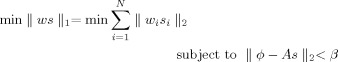
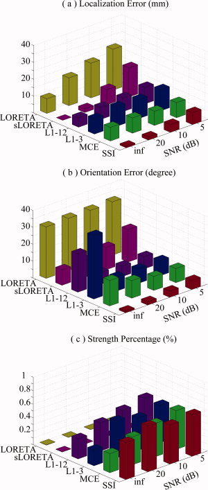
Figure 2 shows the simulation results for the noiseless case using five different L1‐norm GMNEs. The lower quartile, median, and upper quartile of the localization error for SSI is zero and only four voxels show some errors (the Whisker plots in Fig. 2b). Its orientation error is also ∼0°. For the other algorithms, all show the larger localization and orientation errors. The MCE algorithm shows the similar performance using either LORETA or MNE in the first step. The localization errors of L1‐3 and L1‐12 are at the similar level as MCE with the slightly better accuracy of L1‐12 compared with L1‐3. On the other hand, the improvement of orientation estimation by L1‐12 is quite obvious. However, their orientation errors are larger than those from MCE. The errors from different L1‐norm GMNEs seem to exhibit different patterns, with MCE showing obvious depth‐dependence, L1‐3 and L1‐12 showing slight depth‐dependence, and no observed depth‐dependence for SSI. The depth‐dependencies for localization and orientation errors seem to be reversed, especially for MCE. Such observations are further quantitatively analyzed with ANOVA and discussed in the simulation studies with noise below. The strength percentages show that SSI has a much more focused energy distribution as compared with the other four algorithms. Because there is no noise simulated in this condition, the increased errors of source locations and orientations and the decreased energy concentrations in L1‐3 and L1‐12 as compared with SSI must be caused by the inaccurate sparse source field modeling. In MCE, errors are believed to be caused by nonzero systematic bias from L2‐norm GMNEs, even without noise.

Figure 2.

(a) Three evaluation metrics, i.e., localization error (1st row), orientation error (2nd row), and strength percentage (3rd row), of five L1‐norm GMNEs in noiseless case. The simulated sources were at voxels on a selected slice along z‐axis. (b) Whisker plots for three metrics obtained from the simulation results shown in (a) with total 372 samples. [Color figure can be viewed in the online issue, which is available at www.interscience.wiley.com.]

SSI in Noisy Case

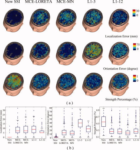
Figure 3 shows the localization errors, orientation errors, and strength percentages of four algorithms (SSI, MCE, L1‐3, and L1‐12) in the presence of noise with SNR of 20 dB using Whisker plots. MCE represents for MCE‐LORETA here. Similar to the noiseless case, SSI still exhibits the lowest localization error (Fig. 3a), the lowest orientation error (Fig. 3c), and the highest energy concentration (Fig. 3d). It is obvious that the localization accuracies are improved in the 2nd step by using the orientations obtained in the 1st step for all four algorithms. A three‐way ANOVA analysis (independent variables are METHOD, SNR, and DEPTH) with more data from different SNRs (shown in Fig. 5) shows statistical significance on the factor METHOD (F = 282.69, n = 3, P < 0.0000). The confidence intervals of localization errors for different methods at a significant level of 0.01 (Duncan correction) revealed by the post hoc test show that the localization error of SSI is significantly lower than the other algorithms (Fig. 3b). While L1‐3 shows the largest localization error, MCE and L1‐12 do not show a significant difference.

Figure 3.

(a) Localization errors for four different L1‐norm GMNEs in two consecutive steps with noise. (b) Plot for factor METHOD produced by post hoc test (Duncan at 0.01) in a three‐way ANOVA analysis. (c) Orientation errors (degree). (d) Strength percentage (%). [Color figure can be viewed in the online issue, which is available at www.interscience.wiley.com.]

Figure 5.

Effects of noise at different SNRs for L1‐ and L2‐norm GMNEs. (a) Mean localization error. (b) Mean orientation error. (c) Mean strength percentage. [Color figure can be viewed in the online issue, which is available at www.interscience.wiley.com.]

Effect of the Size of Solution Space

Although the performance improvements of all L1‐norm GMNEs from the 1st step to the 2nd step have been observed in Figure 3, Figure 4 shows the confidence intervals of localization errors for different sizes of solution spaces in two consecutive steps (Duncan at 0.01), which might explain why the improvements occur. While there are 17,814 unknowns in the optimization problem of the 1st step, the number of unknowns is reduced by three times (5,938, the number of voxels) in the 2nd step using the estimated orientations in the 1st step. In noiseless cases (Fig. 4a), only L1‐3 shows the significant dependence on the factor SSS and, in noisy cases (Fig. 4b), all three algorithms (SSI, L1‐12, L1‐3) show the great dependence on the factor SSS.

Figure 4.

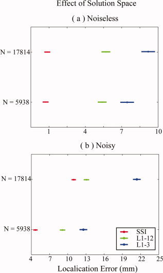
Effects of the size of solution space. (a) Noiseless case; plots are produced by post hoc test (Duncan at 0.01) in a two‐way ANOVA analysis. (b) Noisy case; plots are produced by post hoc test (Duncan at 0.01) in a three‐way ANOVA analysis. [Color figure can be viewed in the online issue, which is available at www.interscience.wiley.com.]

Effect of SNR

A three‐way ANOVA analysis on localization errors (independent variables are METHOD, SNR, and DEPTH) shows the significant effects of factor METHOD (F = 495.67, n = 5, P < 0.0000) and factor SNR (F = 371.08, n = 2, P < 0.0000) among different L1‐ and L2‐norm GMNEs (see Fig. 5). The post hoc test (Duncan at 0.01) indicates that the localization error of SSI is significantly lower than the localization errors of the other five algorithms at every SNR level. Although there is no systematic bias of sLORETA in the noiseless case, its localization error increases much faster than SSI when SNR decreases. The increases of the localization errors in L1‐3 and L1‐12 are not as obvious as SSI when SNR decreases. It may be due to the fact that the errors caused by noises and the orientation discrepancy are not additive. In the conditions of high SNR values, the error due to orientation discrepancy dominates the performance of these two algorithms. A similar phenomenon is observed in MCE which may be caused by the relative poor source imaging accuracy of the L2‐norm GMNE (i.e., LORETA here) in the 1st step, even in the noiseless condition or in the conditions of high SNRs (e.g., 20 dB).

The ANOVA analysis on orientation errors shows significantly the effects of factors METHOD (F = 302.95, n = 5, P < 0.0000) and SNR (F = 14.9, n = 2, P < 0.0000). Among all algorithms, SSI exhibits the significantly lowest orientation error at every noise level. The post hoc test (Duncan at 0.01) indicates that the orientation errors of L1‐norm GMNEs (SSI, MCE, L1‐3, and L1‐12) are significantly smaller than those of L2‐norm GMNEs (LORETA and sLORETA) in noisy conditions. It is interesting that the orientation errors of MCE, L1‐3, and L1‐12 in the noiseless case are significantly (Duncan at 0.01) larger than the cases with noise, which must be caused by the over fit to scalp EEG data in the noiseless case without proper regularization to accommodate the model noise caused by the orientation discrepancy. Comparing the orientation errors of L1‐3 and L1‐12, the latter shows relatively smaller values because it allows more possible orientations (12 versus 6). The large orientation error of MCE may originate from the poor orientation estimation accuracy of LORETA in its first step.

SSI shows significantly (F = 125.46, n = 3, P < 0.0000) concentrated energy in these four L1‐norm GMNEs. The energy distributions for the L2‐norm GMNEs are always smoothed (Fig. 5c).

Dependence Between Source Localization and Orientation Estimates

Figure 6 shows the dependence between the localization error and orientation error for the noiseless case (Fig. 6a) and for the noisy case with a SNR of 20 dB (Fig. 6b). The sources at simulated voxels are each represented by a small dot with different colors for different L1‐norm GMNEs. The dots belonging to the same algorithm are modeled by linear regression and the results are plotted with colored lines. These lines are defined by two parameters: intercept (β ₁) and slope (β ₂). The null hypothesis of whether β ₁ and β ₂ were equal to zero was tested by t‐test [DeGroot and Schervish,2002]. β ₁ not equal to zero means that orientation error is present, even if there is no localization error. β ₂ not equal to zero indicates that there is significant dependence between the localization error and orientation error. The null hypothesis was rejected (P < 0.0000) against both β ₁ and β ₂ in all cases. But comparing the actual β ₁ values, SSI has the lowest intercept, which confirms that SSI has the best orientation estimation accuracy as discussed in the previous section. Similar slope values for all algorithms, especially in the noisy case, indicate the errors for location and orientation estimates are correlated. The larger localization errors normally occur with larger orientation biases.

Figure 6.

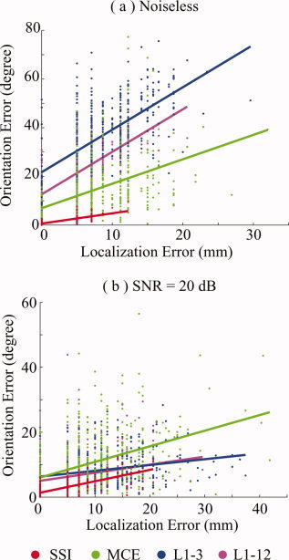
Interdependence of the localization error and orientation error for SSI, MCE, L1‐3, and L1‐12 in (a) noiseless case; and (b) noisy case at SNR = 20 dB. [Color figure can be viewed in the online issue, which is available at www.interscience.wiley.com.]

Dependence of Imaging Accuracy in 2nd Step on Accuracy in 1st Step

In Figure 7, we present the data that examine the dependence of imaging accuracy in the 2nd step based upon the accuracy in the 1st step using the same t‐test as described in the previous section. We used the orientation error at the reconstructed source voxel as the index to measure the imaging accuracy of the 1st step and investigated the dependence of both localization and orientation errors of the 2nd step on this index. The β ₂ values for all curves in Figure 7 are significantly larger than zero (P < 0.001) which confirms that the imaging accuracy of the 2nd step is dependent upon the orientation estimation accuracy of the 1st step. The t‐test shows that only SSI has zero β ₁ for the localization error and the lowest β ₁ value for the orientation error. However, the small orientation errors in the 1st step for the other three algorithms can lead to the large localization error in the 2nd step due to the relative large β ₁ value.

Figure 7.

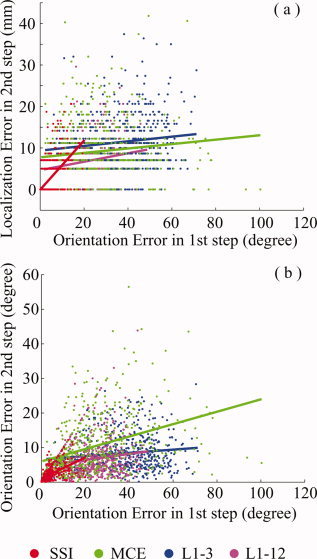
Dependence of the imaging accuracies, i.e., (a) localization accuracy, and (b) orientation accuracy, of the 2nd step on the accuracy of the 1st step for SSI, MCE, L1‐3, and L1‐12. [Color figure can be viewed in the online issue, which is available at www.interscience.wiley.com.]

Effect of Depth

According to the three‐way ANOVA analysis discussed earlier, in which the simulated sources were categorized into three groups (i.e., superficial, middle, and deep) based on their distances to the cortical surface, the significant effects were observed by the factor DEPTH on the localization errors (F = 57.41, n = 2, P < 0.0000) and orientation errors (F = 273.46, n = 2, P < 0.0000). For different algorithms, the depth‐dependence patterns seemed to be quite different. For most algorithms (see Fig. 8), the localization error increases as the simulated source deepens, while the orientation error increases when the simulated source becomes superficial. The slight depth‐dependence of localization error of SSI is not as significant as the depth‐dependencies of L1‐3 and L1‐12. The depth‐dependence of localization error of MCE is more complicated, which may be caused by the contrary depth‐dependencies of the localization error and orientation error. In the 1st step of MCE, LORETA shows the most significant depth‐dependence of orientation error (Duncan at 0.01) (Fig. 8c) as compared with the other L1‐norm GMNEs. Thus, this represents a significant influence on the localization error in the 2nd step of MCE.

Figure 8.

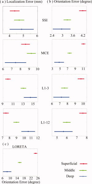
Effects of source depth for four L1‐norm GMNEs. Plots are produced by post hoc test (Duncan at 0.01) in a three‐way ANOVA analysis. (a) Localization error. (b) Orientation error. (c) Orientation error of LORETA as the 1st step of MCE. [Color figure can be viewed in the online issue, which is available at www.interscience.wiley.com.]

Effect of Multiple Current Sources

Figure 9 shows the performance of the six GMNE algorithms with multiple current sources (2, 3, and 5). A two‐way ANOVA analysis on localization errors (independent variables are METHOD and NUMBER) shows the significant effects of the factor METHOD (F = 90.02, n = 5, P < 0.0000) and by factor NUMBER (F = 195.84, n = 2, P < 0.0000). The post hoc test (Duncan at 0.01) (Fig. 9d) indicates that the localization errors of SSI, MCE, and L1‐12 are significantly lower than these of the other algorithms. Although there is no significant difference among SSI, MCE, and L1‐12, SSI is still the one with the smallest localization error (Fig. 9d). It may be due to the fact that the error caused by number of sources dominates over the error due to orientation discrepancy which makes the error differences, among different algorithms, smaller. The ANOVA analysis shows the significant effects of the factors METHOD (F = 514.13, n = 5, P < 0.0000) and NUMBER (F = 545.55, n = 2, P < 0.0000) on the orientation error. Furthermore, the post hoc test (Duncan at 0.01) suggests that SSI has the significantly lower orientation error in all algorithms (Fig. 9e). It also indicates that the orientation errors of L1‐norm GMNEs are significantly smaller than those of L2‐norm GMNEs. The ANOVA analysis further shows that SSI and MCE have similar energy concentrations, which are higher than those of L1‐3 and L1‐12.

Figure 9.

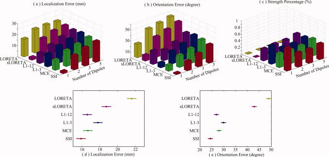
Effects of number of sources for L1‐ and L2‐norm GMNEs. (a) Mean localization error. (b) Mean orientation error. (c) Mean strength percentage. [Color figure can be viewed in the online issue, which is available at www.interscience.wiley.com.]

Algorithm Evaluation in Human Experimentation

Six algorithms (SSI, MCE, L1‐3, L1‐12, sLORETA, LORETA) were applied to the SEP data at its N/P30 component, 30 ms after the stimulus. All of the algorithms showed strong activity in the contralateral sensory‐motor cortex as indicated by the subdural SEP recording (Fig. 10a). We identified the voxel with maximal current source strength in the sensory‐motor cortex as the location of current dipole generating the bipolar potential pattern of N/P30 component in the subdural SEP. These current dipoles from all algorithms are clustered at the posterior edge of subdural ECoG grid, which is close to the central sulcus (CS) (Fig. 10a). It can be observed that there are small discrepancies between the different algorithms for both the estimated locations and orientations. Structurally, the current dipole from SSI is located on the CS. The dipole from MCE appears to be more posterior and the dipoles from L1‐3, L1‐12, sLORETA, and LORETA appear to be more anterior and mesial. To make a quantitative comparison, we calculated the potential fields defined on the subdural ECoG electrodes by two methods. In the first method, we only used the current dipole of maximal activity, as identified earlier to calculate the subdural potentials by solving the forward problem (Fig. 10, left column); and in the second method, the current dipoles at all voxels in the solution space, i.e., the current density distribution, were used to calculate the subdural potentials (Fig. 10, right column). The subdural potential field generated by the dipole from SSI has the most similar pattern to the ECoG recordings suggested by the highest coefficient correlation (CC), i.e., above 0.8. For the other algorithms, in the potentials reconstructed from the dipole with the maximal activity, the maximal potential positivity and negativity are shifted possibly due to the inaccurate location estimations (Fig. 10d,f,g). The obvious rotation and asymmetric strengths of the associated pattern between positivity and negativity should be caused by the inaccurate orientation estimations (Fig. 10c,e,f). The CC values from the other algorithms range between 0.5 and 0.6 which is significantly lower than the CC value from SSI. In the potentials reconstructed from the current density distribution, the improvements in MCE, LORETA, and sLORETA are very obvious. It indicates that the inherited smooth nature of L2‐norm GMNEs, and that the accurate potential field predictions from them need more distributed current density, even though the real source is not distributed (as in this case where the neural generators are considered to be focal instead of distributed [Towle et al.,2003]). Furthermore, the separation between the maximal positivity and maximal negativity in the results from L2‐norm GMNEs seems bigger than the subdural recording (Fig. 10a) and the result from SSI (Fig. 10b), which also reflects their smoothness. The improvement in MCE is possibly due to the same reason, which is caused by the L2‐norm estimation in its first step.

Figure 10.

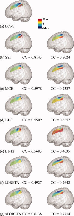
Source imaging results using human SEP data obtained in six algorithms. (a) Subdural SEP recordings and the imaged sources at the voxels within the sensory‐motor cortex with maximal activity from six algorithms (spheres: locations of these voxels; bars: orientations of sources at these voxels; different colors for different algorithms). The predicted subdural SEP by (b) SSI, (c) MCE, (d) L1‐3, (e) L1‐12, (f) LORETA, and (g) sLORETA using two different methods. One used the single dipole source at the voxel with maximal activity (left column); and another used the entire current density distribution (right column). [Color figure can be viewed in the online issue, which is available at www.interscience.wiley.com.]

DISCUSSION

Sparseness Regularization

The L1‐norm GMNE introduces an exponential a priori source field into the inverse problem based upon the distributed current density model. Such regularization, i.e. the sparseness regularization, leads to SSI as opposed to the smooth source imaging achieved by L2‐norm GMNEs. The L2‐norm GMNEs usually give an inverse solution with a highly dispersed energy distribution (less than 0.01% energy concentration at the imaged source voxel) as shown in Figures 3d and 5c. In other simulation studies, its smooth characteristics have been illustrated, e.g. LORETA [Ding et al.,2005], and evaluated quantitatively using crosstalk and point spread metrics [Liu et al.,2002]. The conservative average crosstalk and point spread values of 5–10% from Liu et al. [1998] study indicated the similar energy concentration (i.e., 0.01%). Liu et al. [1998] used an inverse solution regularized by fMRI data that can significantly reduce the crosstalk and point spread, which, however, could not change the smooth nature of L2‐norm GMNEs. The sparse nature of the L1‐norm GMNE is thus attractive, especially, in the inverse source imaging constrained by fMRI. Its lesser popularity as compared with the L2‐norm GMNE may be due to two reasons. The first is the similar source localization accuracy as L2‐norm GMNEs in previously reported L1‐norm GMNEs (Fig. 3a for the 1st step). The second reason is its relative difficulty in solving a nonlinear optimization problem due to the use of the L1‐norm while the L2‐norm GMNE can basically be solved by a linear operator. In the present study, we have introduced a new method to accurately model a sparse source field which corrects the orientation discrepancy in other L1‐norm GMNEs (see Fig. 2). We have further implemented a novel nonlinear optimization solver, i.e. SOCP, to obtain its mathematical solution. In the present study, the L1‐norm GMNE shows significant improvements in location and orientation estimations as compared with the L2‐norm GMNE in both simulations (Figs. 5 and 9) and experimental data analysis (see Fig. 10).

In previously reported L1‐norm GMNEs [Matsuura and Okabe,1995; Uutela et al.,1999; Wagner et al.,1998], the concept of sparseness regularization has not been fully interpreted. The L1‐norm was only mathematically implemented to replace the L2‐norm and the sparseness of the inverse solution was then observed. In some studies [Fuchs et al.,1999], the L1‐norm was not only applied to the regularization term, but also to the data term in Eq. (2). However, the sparse constraint on the noise field which is defined by the data term appears inappropriate since it is unusual that the measurement noise is sparsely distributed or focused on several channels instead of approximately homogeneously distributed over all channels. To distinguish the present algorithm from other L1‐norm algorithms, we term it SSI as interpreted from the Bayesian theory. In the present study, the performance of the new SSI is dependent upon the size of solution space (see Fig. 4), noise level (see Fig. 5), and number of sources (see Fig. 9). However, unlike the other algorithms, it is not depth‐dependent (see Fig. 10). The new SSI also has the most concentrated energy (Figs. 2, 3, and 5) which indicates that it suffers less from the false peak problem. Furthermore, in cases with multiple sources, the error caused by the orientation discrepancy is dominated by the error due to the increased number of sources. The advantage of SSI over other L1‐norm GMNEs thus becomes less significant (see Fig. 9).

Orientation Consideration and Estimation in L1‐ and L2‐Norm GMNEs

In various L1‐norm GMNEs, L1‐3 and L1‐12 show larger orientation errors than SSI in both the simulation and experimental data. This shall be caused by the inaccurate orientation consideration in these two algorithms. As shown in Fig. 10, prediction of the potential field generated by cortical sources depends not only on the accurate estimation of source locations, but also on the accurate estimation of source orientations. The sources imaged by L1‐3 and L1‐12 responsible for the N/P30 potential seem to be more radially oriented to the local curvature of cortical surface as compared with the more tangentially oriented sources imaged by SSI. Because the sparseness a priori in L1‐3 and L1‐12 is applied to the source components at each voxel, the orientations of imaged sources are aligned to the coordinate axes as closely as possible. Thus, the preferred orientations of L1‐3 and L1‐12 are limited which introduces the orientation discrepancy as witnessed in the noiseless case (see Fig. 2) and less so in the noisy cases due to regularization (Figs. 3 and 5). The large orientation error leads to the large localization error in the MCE, L1‐3, and L1‐12 algorithms (Figs. 2, 3, and 5) because of the interdependence of these two types of errors as indicated in Fig. 6. The performance improvement from L1‐3 to L1‐12 is due to the greater number of allowed source orientations. It is worth to point out that the L2‐norm GMNE did not produce accurate orientation estimations, e.g. >30° in all noise levels for LORETA (Figs. 5 and 9b), which may be due to the smooth regularization. Comparing the subdural potentials reconstructed by a single current dipole in the voxel of maximal activity with these by the entire current density distribution, the present results suggest that the voxel of maximal activity in a smooth source distribution from L2‐norm GMNEs may be a reasonable estimate for source location, but not a good estimate for source orientation.

Size of Solution Space

Although the two‐step procedure was first introduced to estimate source orientations at each voxel by MCE [Uutela et al.,1999], we have found that such a two‐step procedure is also helpful in reducing the localization error (Fig. 3a), orientation error (Fig. 3c), and possibility of false peaks (Fig. 3d) for SSI, L1‐3, and L1‐12. The reason for this is that the second step has a smaller‐sized solution space than the first step (i.e., three times). The performance dependence of SSI on the size of the solution space is suggested by simulation in noisy cases (see Fig. 4), which indicates that this effect is closely related to the regularization. The ill‐posedness in underdetermined problem becomes more severe when the number of unknowns increases dramatically. By significantly reducing the number of unknowns from the first step to the second, the regularization becomes more efficient in controlling the ill‐posedness. Figure 7 shows significant dependence of the accuracy of the L1‐norm GMNE in the second step on the accuracy in the first step. The SSI algorithm exhibits the lowest orientation estimation error in the first step (Fig. 3c), and thus has the highest accuracy in location and orientation estimations in the second step (Fig. 3a,c). Such a two‐step procedure implies that SSI can be realized iteratively. First, a coarse grid of voxels can be formed to approximately represent the solution space. The grid can then be iteratively updated to reduce source representation error due to the coarse grid by refining the local neighborhood of voxels exhibiting activity and abandoning voxels without activity to keep the size of the solution space as small as possible. More interestingly, the solution space can be further constrained using prior information from other imaging modalities such as fMRI.

Second‐Order Cone Programming

SOCP, like LP, is an efficient and globally convergent algorithm to solve the sparseness regularization problem in the presence of the L1‐norm. The use of SOCP is due to the presence of nonlinear terms in Eq. (3), while LP can only handle linear equalities or inequalities. The most important advantage of sparseness regularization, i.e., strong sparseness of the inverse solution, is reserved in SOCP as it is in LP. Furthermore, due to the same reason, the selection of regularization parameters was approximated by LP in L1‐3, L1‐12 [Fuchs et al.,1999], and MCE [Uutela et al.,1999]. In SOCP, we used the discrepancy principle [Morozov,1966] in all L1‐ and L2‐norm GMNEs. One limitation of the present SSI is that there is no limit to the strength of the current source at each voxel, which possibly makes the source estimation over focused. And, in the present study, we only investigated the source configurations with their complexity defined by the number of sources, not the source extent. However, the lower and upper limits to the source strength can be applied by introducing additional inequalities in SOCP as discussed in Appendix. These lower and upper limits can be found using the reported estimates of dipole moment density on the cortical surface which is based upon electrophysiological measurements generally ranging between 25 and 250 pAm/mm² [e.g., Hämäläinen et al.,1993]. These values can also be introduced as additional constraints, which will not allow the single dipole at each voxel of unlimited strength and make sparse source reconstruction with each source of certain extent possible. The ability of SOCP to incorporate more constraints gives additional flexibility to the current SSI in order to take advantage of prior information as compared with the relatively fixed linear operators that are popular in L2‐norm GMNEs.

CONCLUSIONS

In the present study, we have introduced the concept of sparseness regularization achieved using the L1‐norm in GMNE. From the Bayesian theory, the L1‐norm could be interpreted as exponential a priori source field modeling which results in strong sparseness of the inverse solution. Based upon this framework, we have developed a new SSI method by accurately modeling the sparse source field. The new SSI was studied by a series of simulations and evaluated using human SEP experimental data with subdural recordings as compared with other various L1‐ and L2‐norm GMNEs. The present simulation results indicate that the new SSI has significantly improved performance in the estimations of source location and orientation. The human evaluation study using independent subdural measurements further confirms that the new SSI has the best prediction of the subdural potential field in the SEP protocol. Most attractive about the new SSI is the strong sparseness of inverse solution as well as the flexibility of solver (i.e., SOCP) which is able to incorporate many physiologically meaningful priors for the purpose of multimodal imaging. While we examined the performance of SSI in EEG source imaging, the proposed SSI concept and algorithm should also be applicable to MEG source imaging.

Second‐Order Cone Programming and Its Implementation in SSI

Although the L1‐norm regularized inverse imaging problem has a convex cost function, the solution is by no means trivial. This is because the cost function is neither linear nor quadratic when the L1‐norm appears for vector data. Such a problem cannot be formulated as LP or quadratic programming. Fortunately, the use of the L1‐norm for vector data can be reformulated as SOCP [Nemirovski and Ben Tal,2001] which has an efficient globally convergent solver known as the interior point methods. This method has been implemented in a MATLAB package named SeDuMi (which stands for self‐dual‐minimization) [Sturm,2001]. Since the methods to solve SOCP problems have been intensively studied theoretically and implemented practically, we will focus our discussions on what kind of problems can be solved by the SOCP and how to reformulate the SSI problem into the framework of SOCP.

SOCP explicitly deals with the constraints of form ‖ x ₂, … x _n ‖₂ ≤ | x ₁| which are known as the Lorentz cone [Nemirovski and Ben Tal,2001] if x = [x ₁, x ₂, …, x _n]^T is the solution vector for a SOCP problem. SOCP has two standard forms over a pair of so‐called selfdual homogeneous cones, i.e., the primal form (left) and the dual form (right):

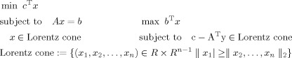(A1)

where b and c are the coefficient vectors and A is the coefficient matrix, which are defined specifically in each given problem. SeDuMi implements the selfdual embedding technique [Sturm,2001] for optimization over the selfdual homogeneous cones defined above and estimates values for the solution vector, x. Note that the solution vector, x, here is not the same as the source vector, s, in Eqs. (3) and (4) from SSI. The Eq. (A1) expresses the standard forms of a SOCP problem which could be solved by SeDuMi while the SSI problems formulated in Eqs. (3) and (4) are not in such standard forms yet. Certain intermediate variables need to be introduced in order to reformulate a SSI problem into a SOCP problem. The solution vector therefore consists of the source vector and the intermediate variables introduced during the problem reformulation. The SSI problem can be reformulated into either the primal form or the dual form and, here, we use the primal form to represent the problem without noise:

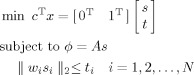(A2)

where the coefficient vector c = 1^T and b = ϕ, and the coefficient matrix A is the lead field defined in Eq. (1). The solution vector is defined as x = [s ^T t ^T]^T and ‖ w _i s _i‖₂≤ t _i is the Lorentz cone defined for the second‐order cone constraints where t is the introduced intermediate variable. Note that there are multiple Lorentz cones with each one only involving a dipole at each voxel. Each Lorentz cone constrains the weighted L2‐norm of each dipole element, as defined in Eq. (4), to an intermediate variable t_i and the L1‐norm of the source vector s is minimized by summing all t_i. Note that all equalities or inequalities in the standard form, i.e. Eq. (A1), involves every element of the solution vector, x, which may not be true in the realization of a specific problem, e.g. Eq. (A2). A practical way is to assign zero values to the coefficients in A, b, and c corresponding to the uninvolved elements. In Eq. (A2), those uninvolved elements are simply ignored to keep it easy for understanding.

The SSI problem with the presence of noise can be similarly formed as

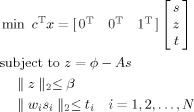(A3)

The solution vector x = [s ^T z ^T t ^T]^T, where z and t are intermediate variables. t is a vector with each element representing the weighted amplitude of dipole source at each voxel as in Eq. (A2), while z represents the measurement error vector. The introduction of z splits the nonlinear constraint, ‖ ϕ − As ‖₂ < β, into the linear constraint, z = ϕ − As, and the second order cone constraint, ‖ z ‖₂ < β, which are standard forms for a SOCP problem. Other formulations are similar as Eq. (A2).

All other L1‐norm GMNEs studied in the article can be formulated similarly as a SOCP problem which can be solved by SeDuMi. Note that SOCP formulations were used for all L1‐norm GMNE algorithms since they used the same regularization method which required a Lorentz cone representation. The regularization method is discussed in the Regularization Parameter Selection section.

REFERENCES

- Baillet S, Garnero L ( 1997): A Bayesian approach to introducing anatomo‐functional priors in the EEG/MEG inverse problem. IEEE Trans Biomed Eng 44: 374–385. [DOI] [PubMed] [Google Scholar]
- Dale AM, Sereno MI ( 1993): Improved localization of cortical activity by combining EEG and MEG with MRI cortical surface reconstruction: A linear approach. J Cogn Neurosci 5: 162–176. [DOI] [PubMed] [Google Scholar]
- DeGroot MH, Schervish MJ ( 2002): Probability and Statistics, 3rd ed. Boston, MA: Addison Wesley. [Google Scholar]
- Ding L, Lai Y, He B ( 2005): Low resolution brain electromagnetic tomography in a realistic geometry head model: A simulation study. Phys Med Biol 50: 45–56. [DOI] [PubMed] [Google Scholar]
- Fuchs M, Wagner M, Kohler T, Wischmann HA ( 1999): Linear and nonlinear current density reconstructions. J Clin Neurophysiol 16: 267–295. [DOI] [PubMed] [Google Scholar]
- Gorodnitsky IF, George JS, Rao BD ( 1995): Neuromagnetic source imaging with FOCUSS: A recursive weighted minimum norm algorithm. Electroencephalogr Clin Neurophysiol 95: 231–251. [DOI] [PubMed] [Google Scholar]
- Hämäläinen MS, Ilmoniemi RJ ( 1984): Interpreting measured magnetic fields of the brain: Estimates of current distributions. Technical Report TKK‐F‐A559, Helsinki University of Technology.
- Hämäläinen M, Sarvas J ( 1989): Realistic conductor geometry model of the human head for interpretation of neuromagnetic data. IEEE Trans Biomed Eng 36: 165–171. [DOI] [PubMed] [Google Scholar]
- Hämäläinen MS, Hari R, Ilmoniemi RJ, Knuutila J, Lounasmaa OV ( 1993): Magnetoencephalography—Theory, instrumentation, and applications to noninvasive studies of the working human brain. Rev Mod Phys 65: 413–497. [Google Scholar]
- Hann H, Streb J, Bien S, Rösler F ( 2000): Individual cortical current density reconstructions of the semantic N400 effect: Using a generalized minimum norm model with different constraints (L1 and L2 norm). Hum Brain Mapp 11: 178–192. [DOI] [PMC free article] [PubMed] [Google Scholar]
- He B ( 1999): Brain electric source imaging: Scalp Laplacian mapping and cortical imaging. Crit Rev Biomed Eng 27: 149–188. [PubMed] [Google Scholar]
- He B, Lian J ( 2005): Electrophysiological neuroimaging In: He B, editor. Neural Engineering. London, UK: Kluwer Publishers; pp 221–262. [Google Scholar]
- He B, Musha T, Okamoto Y, Homm S, Nakajima Y, Sato T ( 1987): Electrical dipole tracing in the brain by means of the boundary element method and its accuracy. IEEE Trans Biomed Eng 34: 406–414. [DOI] [PubMed] [Google Scholar]
- He B, Yao D, Lian J, Wu D ( 2002a): An equivalent current source model and Laplacian weighted minimum norm current estimates of brain electrical activity. IEEE Trans Biomed Eng 49: 277–288. [DOI] [PubMed] [Google Scholar]
- He B, Zhang X, Lian J, Sasaki H, Wu D, Towle VL ( 2002b): Boundary element method based cortical potential imaging of somatosensory evoked potentials using subjects' magnetic resonance images. Neuroimage 16: 564–576. [DOI] [PubMed] [Google Scholar]
- Henderson CJ, Butler SR, Glass A ( 1975): The localization of equivalent dipoles of EEG sources by the application of electrical field theory. Electroenceph Clin Neurophysiol 39: 117–130. [DOI] [PubMed] [Google Scholar]
- Jeffs B, Leahy R, Singh M ( 1987): An evaluation of methods for neuromagnetic image reconstruction. IEEE Trans Biomed Eng 34: 713–723. [DOI] [PubMed] [Google Scholar]
- Liu AK, Belliveau JW, Dale AM ( 1998): Spatiotemporal imaging of human brain activity using fMRI constrained MEG data: Monte Carlo simulations. Proc Natl Acad Sci USA 95: 8945–8950. [DOI] [PMC free article] [PubMed] [Google Scholar]
- Liu AK, Dale AM, Belliveau JW ( 2002): Monte Carlo simulation studies of EEG and MEG localization accuracy. Hum Brain Mapp 16: 47–62. [DOI] [PMC free article] [PubMed] [Google Scholar]
- Matsuura K, Okabe Y ( 1995): Selective minimum‐norm solution of the biomagnetic inverse problem. IEEE Trans Biomed Eng 42: 608–615. [DOI] [PubMed] [Google Scholar]
- Metz CE, Fencil LE ( 1989): Determination of three‐dimensional structure in biplane radiography without prior knowledge of the relationship between the two views: Theory. Med Phys 16: 45–51. [DOI] [PubMed] [Google Scholar]
- Morozov AV ( 1966): On the solution of functional equations by the method of regularization. Soviet Math Dokl 7: 414–417. [Google Scholar]
- Nemirovski A, Ben Tal A ( 2001): Lectures on Modern Convex Optimization Analysis, Algorithms and Engineering Application, SIAM. Philadelphia, US: Society for Industrial & Applied Mathematics (SIAM). [Google Scholar]
- Nunez PL, Srinivasan R ( 2005): Electric Fields of the Brain: The Neurophysics of EEG, 2nd ed. USA: Oxford University Press. [Google Scholar]
- Pascual‐Marqui RD ( 2002): Standardized low resolution brain electromagnetic tomography (sLORETA): Technical detail. Methods Find Exp Clin Pharmacol 24D: 5–12. [PubMed] [Google Scholar]
- Pascual‐Marqui RD, Michel CM, Lehmann D ( 1994): Low resolution electromagnetic tomography: A new method for localizing electrical activity in the brain. Int J Psychophysiol 18: 49–65. [DOI] [PubMed] [Google Scholar]
- Pulvermüller F, Shtyrov Y, Ilmoniemi R ( 2003): Spatiotemporal dynamics of neural language processing: An MEG study using minimum‐norm current estimates. Neuroimage 20: 1020–1025. [DOI] [PubMed] [Google Scholar]
- Sidman RD, Giambalvo V, Allison T, Bergey P ( 1978): A method for localization of sources of human cerebral potentials evoked by sensory stimuli. Sens Process 2: 116–129. [PubMed] [Google Scholar]
- Silva C, Maltez JC, Trindade E, Arriaga A, Ducla‐Soares E ( 2004): Evaluation of L1 and L2 minimum norm performances on EEG localizations. Clin Neurophysiol 115: 1657–1668. [DOI] [PubMed] [Google Scholar]
- Sturm JS ( 2001): Using SeDuMi 1.02, a Matlab toolbox for optimization over symmetric cones. Technical Report, Department of Econometrics, Tilburg University, Netherlands.
- Towle VL, Khorasani L, Uftring S, Pelizzari C, Erickson RK, Spire JP, Hoffmann K, Chu D, Scherg M ( 2003): Noninvasive identification of human central sulcus: A comparison of gyral morphology, functional MRI, dipole localization, and direct cortical mapping. NeuroImage 19: 684–697. [DOI] [PubMed] [Google Scholar]
- Uutela K, Hamalainen M, Somersalo E ( 1999): Visualization of magnetoencephalographic data using minimum current estimates. NeuroImage 10: 173–180. [DOI] [PubMed] [Google Scholar]
- Valeriani M, Le Pera D, Niddam D, Arendt‐Nielsen L, Chen A ( 2000): Dipolar source modeling of somatosensory evoked potentials to painful and nonpainful median nerve stimulation. Muscle Nerve 23: 1194–1203. [DOI] [PubMed] [Google Scholar]
- Wagner M, Wischmann HA, Fuchs M, Kohler T, Drenckhahn R ( 1998): Current density reconstruction using the L1 norm. Advances in Biomagnetism Research: Biomag96. New York: Springer‐Verlag; pp 393–396. [Google Scholar]
- Yao J, Dewald JPA ( 2005): Evaluation of different cortical source localization methods using simulation and experimental EEG data. NeuroImage 25: 369–382. [DOI] [PubMed] [Google Scholar]
- Zhang Y, van Drongelen W, He B ( 2006): Estimation of in vivo human brain‐to‐skull conductivity ratio in humans. Appl Phys Lett 89: 223903. [DOI] [PMC free article] [PubMed] [Google Scholar]