Log Normal Distribution of Cellular Uptake of Radioactivity: Statistical Analysis of Alpha Particle Track Autoradiography

Abstract

Recently, the distribution of radioactivity among a population of cells labeled with ²¹⁰Po was shown to be well described by a log normal distribution function (J Nucl Med 47, 6 (2006) 1049-1058) with the aid of an autoradiographic approach. To ascertain the influence of Poisson statistics on the interpretation of the autoradiographic data, the present work reports on a detailed statistical analyses of these data.

Methods

The measured distributions of alpha particle tracks per cell were subjected to statistical tests with Poisson (P), log normal (LN), and Poisson – log normal (P – LN) models.

Results

The LN distribution function best describes the distribution of radioactivity among cell populations exposed to 0.52 and 3.8 kBq/mL ²¹⁰Po-citrate. When cells were exposed to 67 kBq/mL, the P – LN distribution function gave a better fit, however, the underlying activity distribution remained log normal.

Conclusions

The present analysis generally provides further support for the use of LN distributions to describe the cellular uptake of radioactivity. Care should be exercised when analyzing autoradiographic data on activity distributions to ensure that Poisson processes do not distort the underlying LN distribution.

INTRODUCTION

Autoradiography has been used for decades to quantify the distribution of radioactivity in tissues following administration of radiochemicals (1-6). Recently, alpha particle track autoradiography was used to determine the distribution of ²¹⁰Po-citrate among a clonal cell population of Chinese hamster V79 lung fibroblasts (7). Analysis of the data revealed a log normal distribution of cellular activity, a distribution that can have a substantial effect on the biological response of the cell population (7,8). To arrive at this distribution, the number of alpha particle tracks per cell was scored in >1000 cells. However, it was necessary to limit the number of counted tracks per cell to less than ten to ensure accurate scoring. The statistical uncertainties associated with measuring these low numbers of tracks per cell can affect the measured track distribution and thereby potentially distort the underlying activity distribution among the cell population (9,10).

As pointed out by Kvinnsland et al. (9), it is the statistical nature of radioactive decay that can influence the measured distribution of alpha particle tracks, particularly at the low numbers of tracks per cell studied by Neti et al. (7). Therefore, it may be necessary to “peel off” the distribution associated with the statistics of radioactive decay in order to arrive at the underlying activity distribution. It has been hypothesized that in radioactive decay, all atoms are identical; independent; and the chance for an atom to disintegrate during a given time interval is the same for all time intervals of equal size. Accordingly, after the discovery of radioactivity, initial experiments suggested that the decay process, and particle counting associated with its observation, are well approximated by simple Poisson processes. Subsequently, while studying α–particle emission rates, a quantum self-interference phenomenon was proposed to account for 1/f fluctuations (11). Experiments showed that α–emission is in fact not a simple Poisson process, and particle counting is not adequately described by Poisson statistics (12). However, there is also a report that 1/f fluctuations are not present in the decay of ²¹⁰Po at decay frequencies in excess of 10⁻⁶ Hz (13). The mean track numbers for the range of ²¹⁰Po-citrate concentrations discussed in the present report fall in the window of ~ 0.16 − 1.6 × 10⁻⁶ Hz. Consequently, it is unlikely that 1/f fluctuations play a significant role in interpreting our experimental alpha particle track data (7). Nevertheless, Poisson statistics may play a role. Therefore, it is necessary to examine whether the log normal distribution obtained from our ²¹⁰Po alpha particle track data is influenced by the Poisson distribution associated with its decay. Accordingly, in this report, we subject our α–particle track data to statistical tests with Poisson (P), log normal (LN) and Poisson-log normal (P – LN) distribution functions (14).

METHODS

Summary of published experimental data and analyses

The methods used to obtain the α–particle track data that are statistically analyzed herein are explained in detail in ref. (7). Briefly, cultured cells were labeled with ²¹⁰Po-citrate, washed, and coated with autoradiographic emulsion. Decays were allowed to accumulate for various times to obtain scoreable track data that covered the entire range of cellular activities encountered in a given labeled cell population. Accordingly, the emulsion was developed for two or three different exposure times. For each emulsion exposure time, 500-1200 cells were examined and the number of tracks in each cell was recorded. Cells with 0-9 tracks per cell were scored as such. Cells with >9 tracks could not be accurately counted and were simply scored as >9 tracks. The entire process was repeated for ²¹⁰Po-citrate labeling concentrations of 0.52, 3.8, and 67 kBq/mL that resulted in mean cellular activities of 0.054, 0.12, and 1.8 mBq/cell, respectively. The numbers of tracks per cell from the short exposure times were decay corrected to the longest exposure time and then normalized. All data sets for a given labeling concentration were then combined into a single convolved track distribution with the longest exposure time data providing the distribution for the lower multiplicity of convolved tracks and the short exposure time data providing the distribution of the higher multiplicity. A nonlinear least squares fit of the resulting convolved track distribution was carried out with a log normal function (7).

Experimental mean number of alpha particle tracks per cell

The arithmetic mean number of tracks per cell <n> can be calculated for the track data corresponding to the shortest emulsion exposure times for each labeling concentration. These data have no cells with > 9 tracks and therefore the mean is obtained by simply tallying the total number of tracks and dividing by the number of cells. A different approach was required to calculate <n> for the data sets corresponding to longer emulsion exposure times that contained cells with > 9 tracks. Regardless of the mathematical nature of the track distribution, the total number of tracks n_total recorded in the cell population at time point t₁ can be projected to a later time point t₂ according to Eq. (1),

$$n_{\mathit{total}}(t_1\Rightarrow t_2)=n_{\mathit{total}}(t_1)\frac{(1-e^{-0.693t_2/T_{\mathrm{p}}})}{(1-e^{-0.693t_1/T_{\mathrm{p}}})}$$ (1)

where T_p is the physical half-life of the radionuclide (T_p = 138 d for ²¹⁰Po). In the same manner, <n(t₁)> (shortest exposure time with all cells having < 9 tracks) can be used to calculate <n(t₂)> (longer exposure time with some cells having > 9 tracks).

Statistical distributions and analyses

Poisson distribution

It is generally accepted that if each cell in the population had the same activity, one would anticipate a Poisson distribution of tracks per cell. There is evidence to suggest that a 1/f distribution may be expected (12), however, there is a report indicating that 1/f fluctuations are not present in the decay of ²¹⁰Po for frequencies in excess of 10 ^{− 6} Hz (13), a frequency range that encompasses our data. Thus, in this report, the Poisson distribution is assumed to adequately describe the statistical distribution associated with the decay of ²¹⁰Po. Given knowledge of <n> for each set of track distribution data, the Poisson probability of n discrete tracks per cell is given by

$${\mathrm{P}}_P(n)=e^{-<n>}\frac{<n{>}^n}{n!}(n=0,1,2,\mathrm{\dots })$$ (2)

For non-integer values of n, which may result due to decay correction (Eq. (1)), truncated values are used to calculate the probability.

Log normal distribution

The log normal (LN) probability density function is given by,

$${\mathrm{P}}_{\mathit{LN}}(n)=\frac{g}{n\mathrm{\sigma }}{e}^{\frac{-{(\ln n-{\text{μ}}_n)}^2}{2{\mathrm{\sigma }}^2}},n>0$$ (3)

where μ_n is the scale parameter, σ is the shape parameter, and g is a constant. The scale parameter is related to the mean according to μ_n = ln<n> - σ²/2. The properties of this function and its use in analysis of the distribution of tracks per cell are given in Ref. (7). Detailed information on log normal distributions can be found in Refs. (15) and (16).

Poisson log normal distribution

The P – LN compound probability of obtaining a realization n and all its possible Poisson realizations k is given by (17),

$${\mathrm{P}}_{P-LN}(n|<n>)=\sum _{k=1}^{\infty }\frac{1}{\sqrt{2\pi }\sigma n}{e}^{-\frac{{\left(\ln \frac{n}{k}-\frac{{\mathrm{\sigma }}^2}{2}\right)}^2}{2{\sigma }^2}}{e}^{-<n>}\frac{<n{>}^n}{n!}$$ (4)

Chi-square analyses

To quantitatively assess which of the above statistical distributions best describe the observed track distribution data, a reduced chi-square analysis (χ̂²) was performed. This quantity is given by Eq. (5),

$${\widehat{\chi }}^2=\frac{1}{v}\sum _{i=1}^{i_{\max }}\frac{{(n_i-n_{\mathrm{expected},i})}^2}{n_i}$$ (5)

where n_i is the number of tracks per cell for the i^th experimental datum, n_expected,i is the expected value based on the assumed distribution, v is the degrees of freedom (v = i_max − p − 1), and p is the number of parameters in the assumed distribution.

Least-squares fit

Least squares (LS) fits of the data to a LN distribution function (Eq. (3)) were performed with Sigmaplot (Systat Software, San Jose, CA). The LS fit of the LN distribution function to the data corresponding to emulsion exposure times where >9 tracks were observed was carried out by two methods: 1) <n> was calculated by decay correcting <n(t₁)> to obtain <n(t₂)>, and then <n(t₂)> was constrained to obtain σ; 2) both <n> and σ were allowed to vary. No constraints were placed on the LS fit of the LN distribution function to the convolved data.

RESULTS

Statistical analysis for cells exposed to 0.52 kBq/mL

To study the effect of Poisson statistics on our analyses, the three discrete raw data sets from Fig. 3A in Ref. (7) (0.52 kBq/mL) are first revisited. The three sets of track distributions were acquired from autoradiographs that were developed at t = 7, 26, and 52 d, as shown in Figure 1A, 1B and 1C, respectively. Each set of track distribution data include the number of cells scored with 0-9 tracks per cell, as well as the number of cells with an unscoreable number of tracks (>9 tracks). The t = 7 d data have a maximum of 6 tracks in any given cell and there are no cells having >9 tracks. The mean value for the t = 7 d data is 1.0 tracks/cell. The values of <n> for t = 26 d and t = 52 d cannot be obtained directly from the respective data sets because some of the cells have >9 tracks. Thus, the projected <n> values, obtained with Eq. (1), are 3.6 and 6.7 for the 26 d and 52 d data, respectively. Using these <n>, the Poisson probabilities for each of 0-9 discrete tracks per cell are calculated at t = 7, 26, and 52 d. These probabilities can be used to assess the extent to which our experimental data represent a Poisson distribution. As shown in Figure 1A, the t = 7 d experimental data follow the general trend of a Poisson distribution which suggests that Poisson statistics may have some impact on these data. The t = 26 d (Figure 1B) and t = 52 d (Figure 1C) data sets do not follow a Poisson distribution, although this does not rule out a Poisson component in these distributions.

Figure 1.

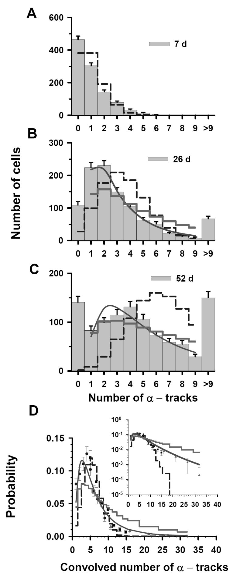
Statistical analysis of α-particle track distribution in V79 lung fibroblasts that were labeled in culture medium containing 0.52 kBq/mL ²¹⁰Po-citrate. The vertical bars with standard errors in panels A, B, and C represent the experimental track distributions (discrete) when scored after decays were allowed to accumulate for 7, 26, and 52 d, respectively (7). The data points in Panel D represent a normalized convolution of the experimental track data obtained at 7 d (▲), 26 d (■), and 52 d (●). Error bars represent standard errors. In each panel, the predicted probabilities, based on Poisson, Poisson-log normal (P – LN), and log normal (LN) functions, are given by the dashed step line, thick solid step line and solid curve, respectively. The parameters of the three probability density functions are enumerated in Table 1. To compare the trends of these probability functions relative to the experimental data at high numbers of convolved tracks, the inset in panel D plots the ordinate on a log scale.

To assess the possible Poisson component, we return to the t = 52 d data set. This is the primary data set, covers the range of 0–9 tracks in our convolved data, and primarily dictates the shape of the probability distribution. For the t = 52 d data, the χ̂² values for the Poisson, LN, and P – LN distributions were 149, 3.2, and 6.5, respectively. The latter two values were obtained via a χ̂² minimization procedure with respect to the shape parameter (σ). The values of σ were 0.81 and 1.1 for the LN and P – LN distributions, respectively. The lowest χ̂² value was obtained for the LN distribution as shown in Table 1, suggesting that Poisson corrections are not required for the t = 52 d data. Furthermore, the σ obtained with the LN distribution corresponding to the discrete t = 52 d data was the same as that obtained by LS fit of the convolved data which included the t = 7, 26, and 52 d data.

TABLE 1.

Statistical analysis of ²¹⁰Po α–particle track distribution data (7) using Poisson, log normal (LN) and Poisson-log normal (P – LN) functions.

Labeling concentration (kBq/mL)†	Exposure Time (d)	Function		<n> ‡ (tracks/cell)	σ §	v	χ̂2	R2
0.52 ± 0.051	52d	Poisson	}	6.7*	—	7	149
		LN			0.81	6	3.2	—
		P – LN			1.1	6	6.5
		Constrained LS fit to LN		6.7* ± 1.1	0.80 ± 0.097	5	3.9	0.78
		LS fit to LN		8.2 ± 1.7	0.88 ± 0.11	6	3.2	0.81
	Convolved (52, 26, 7d)	Poisson	}	5.5	—	19	7.7E+07
		LN			0.71	18	3.6	—
		P – LN			0.96	18	12
		LS fit to LN		7.1 ± 0.63	0.80 ± 0.056	18	3.1	0.92
3.8 ± 0.36	4 d	Poisson	}	7.3*	—	7	25
		LN			0.64	6	0.5	—
		P – LN			0.60	6	1.1
		Constrained LS fit to LN		7.3* ± 0.32	0.61 ± 0.029	5	1.2	0.98
		LS fit to LN		7.4 ± 0.33	0.62 ± 0.029	6	0.9	0.98
	Convolved (0.67, 4d)	Poisson	}	6.1	—	16	1.2E+07
		LN			0.62	15	2.8	—
		P – LN			0.57	15	2.1
		LS fit to LN		6.9 ± 0.22	0.59 ± 0.023	15	1.9	0.98
67 ± 6.6	1 d	Poisson	}	5.7*	—	7	1.1
		LN			0.54	6	5.6	—
		P – LN			0.28	6	0.66
		Constrained LS fit to LN		5.7* ± 0.33	0.48 ± 0.044	5	15	0.88
		LS fit to LN		6.5 ± 0.29	0.52 ± 0.033	6	9.5	0.95
	Convolved (0.25, 1d)	Poisson	}	5.7	—	14	9.6E+06
		LN			0.62	13	8.4	—
		P – LN			0.49	13	1.7
		LS fit to LN		6.7 ± 0.25	0.54 ± 0.029	13	6.3	0.97

^*The arithmetic mean <n> with * is decay corrected for t₂ > t₁, otherwise <n> is obtained from the raw data. σ, v are the log normal shape parameter and degrees of freedom, respectively. The values are shown upto two significant digits.

^†Errors are based on SD of triplicate measurements of scintillation counts and cell counts.

^‡Standard Errors are provided by least-squares fit of the data to a LN function using SigmaPlot (SPSS).

^§Optimized value of σ (shape parameter) obtained via minimization of chi-square (χ̂²) procedure.

Now that the LN distribution has been firmly established with the primary t = 52 d data, we return to the now ancillary t = 7 and 26 d data where the Poisson distribution may play a more significant role. These data represent cells from the tail of the LN distribution and therefore contain little information about the overall shape of the entire activity distribution in the cell population. Accordingly, although a LN distribution with σ = 0.8 fits these data extremely well, it is not appropriate to apply this distribution to this subset of data. For the same reason, the P – LN distribution cannot be used to assess the significance of the Poisson distribution in these data. This makes it difficult to tease the possible Poisson influence out of the underlying distributions in the t = 7 and 26 d data sets. With this limitation in mind, it is worth revisiting the convolved data where these distributions are applicable. The 52 d data were used for the low multiplicity of convolved tracks/cell (1–9 tracks), the 26 d data were used for the middle multiplicity (5–15 tracks), and the 7 d data were used for high multiplicity (10–32 tracks). Importantly, within the overlapping regions (see Fig. 1D), there is considerable agreement between the data points from independent data sets. Furthermore, a χ̂² analysis of the convolved data gives 7.7 × 10⁷, 3.6, and 12 for the Poisson, LN, and P – LN, respectively. The difference between the convolved data and the three predicted probability curves can be seen in the inset of Figure 1D at very small probabilities. Again, the data are best described by the LN distribution (Table 1). This suggests that the convolved t = 7 d and 26 d data follow the expected trend of the LN distribution and any Poisson-component in these data has a negligible impact on the overall distribution.

Statistical analysis for cells exposed to 3.8 kBq/mL

An approach similar to that described above was also applied to the two discrete data sets that were obtained at a labeling concentration of 3.8 kBq/mL. The two sets of track distributions were acquired from autoradiographs that were developed at t = 0.67, and 4 d, as shown in Figure 2A and 2B, respectively. In this case, the t = 4 d data set is the primary data set, covers the range of 0–9 tracks of convolved data, and primarily dictates the shape of the probability distribution. The <n> for the t = 0.67 d data, where all cells have <9 tracks per cell, is 1.2 tracks/cell. The mean number of tracks per cell for the 4 d data can be obtained with Equation (1) which results in <n> = 7.3. The Poisson probabilities for each of 0-9 discrete tracks per cell are calculated for <n> = 1.2 (t = 0.67 d), and 7.3 (t = 4 d) (Figure 2A and 2B). The χ̂² values for the Poisson distribution are 96 and 25 for 0.67 and 4 d data sets, respectively. The χ̂² values for all three distribution functions are given in Table 1. Upon minimization of χ̂² , the values of σ were 0.64 and 0.60 for the LN and P – LN, respectively. The lowest χ̂² value was obtained for the LN distribution (Table 1), thereby again suggesting that Poisson corrections are not required for the t = 4 d data. Furthermore, the σ obtained for the LN distribution corresponding to the t = 4 d data was the same as that obtained by a LS fit to the convolved data. There is good agreement between the data points within the overlapping regions of the convolved data sets (see Fig. 2C). The arithmetic mean (<n>) value of 6.1 for the convolved data set was obtained from a LS fit of the convolved data to the LN distribution. Furthermore, χ̂² analysis of the convolved data gives 1.2 × 10⁷, 2.8, and 2.1 for the Poisson, LN, and P – LN, respectively. The difference between the convolved data and the three predicted probability curves is shown in the inset of Figure 2C. Again, the data is best described by the LS fit of the convolved data to a LN distribution function (Table 1, χ̂² =1.9).

Figure 2.

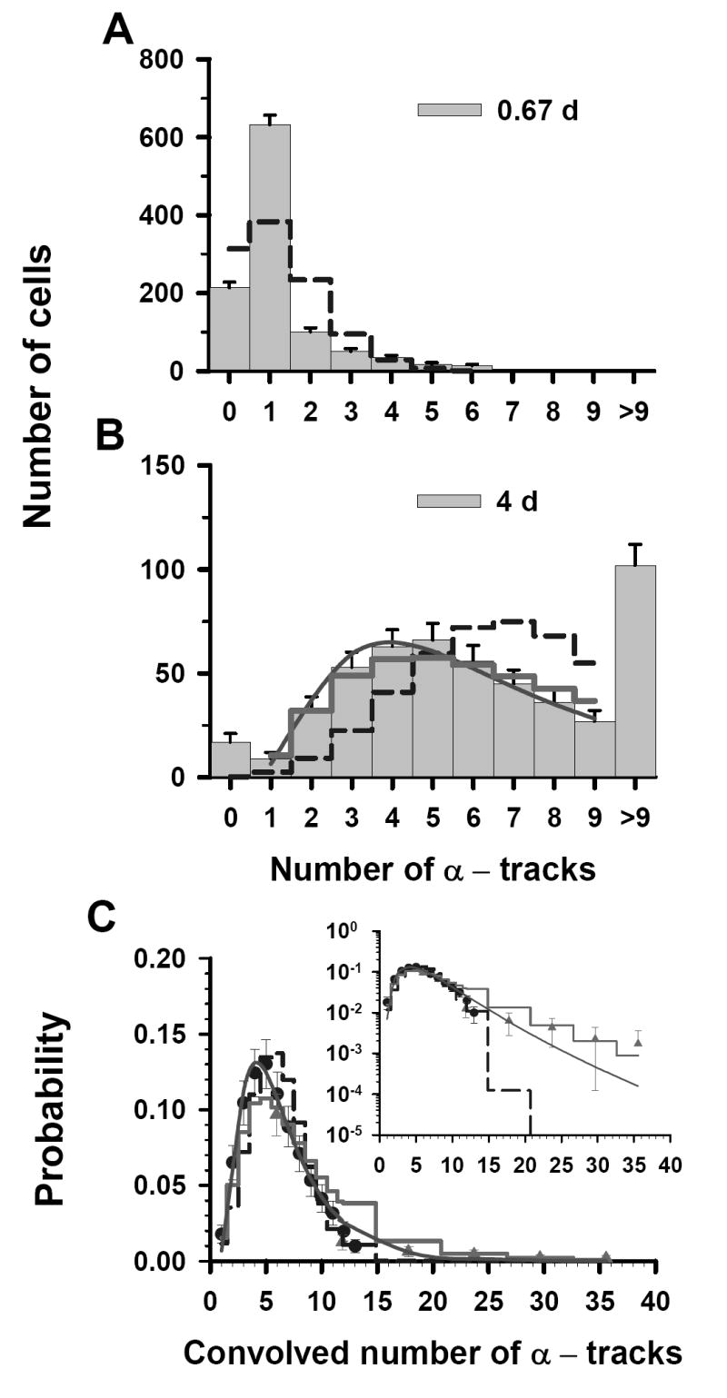
Statistical analysis of α-particle track distribution in V79 lung fibroblasts that were labeled in culture medium containing 3.8 kBq/mL ²¹⁰Po-citrate. Decays were allowed to accumulate for 0.67 d (A) and 4 d (B). The data points in Panel C represent a normalized convolution of the experimental track data obtained at 0.67 d (▲) and 26 d (●). Error bars, dashed step line, thick solid step line, solid curve and the inset are all as explained in Fig. 1. The parameters of the three probability density functions are also enumerated in Table 1.

Statistical analysis for cells exposed to 67 kBq/mL

Finally, the results are somewhat different at the highest labeling concentration 67 kBq/mL. In this case, the two sets of track distributions were acquired from autoradiographs that were developed at t = 0.25, and 1 d (Figs. 3A and 3B). The <n> for the t = 0.25 d data is 1.4 tracks/cell and, using Equation (1), <n> = 5.7 for the 1 d data. The Poisson probabilities for each of 0-9 discrete tracks per cell are calculated with Equation (2) for each <n>. As shown in Figure 3A, the t = 0.25 d data set do not follow a Poisson distribution (χ̂² = 91). However, the t = 1 d data are better described by the Poisson distribution (χ̂² = 1.1) than the LN distribution (χ̂² = 5.6). The P – LN distribution function provides the best fit to the data suggesting a significant Poisson contribution (χ̂² = 0.66). The values of σ were 0.54 and 0.28 for the LN and P – LN, respectively. The σ obtained for the LN distribution corresponding to t = 1 d data was the same as that obtained by LS fit for the convolved data (Table 1). Again, within the overlapping regions, of the convolved data there is considerable agreement between the data points from independent data sets (see Fig. 3C). Furthermore, χ̂² analysis of the convolved data gives 9.6 × 10⁶, 8.4, and 1.7 for the Poisson, LN, and P – LN, respectively. A comparison between the convolved data and the three predicted probability curves is provided in the inset of Figure 3C. The data are much better described by the LS fit of the convolved data to a LN distribution function (Table 1, χ̂² =6.3) than to a Poisson distribution (χ̂² =9.6×10⁶), but best explained by the P – LN model (χ̂² = 1.7).

Figure 3.

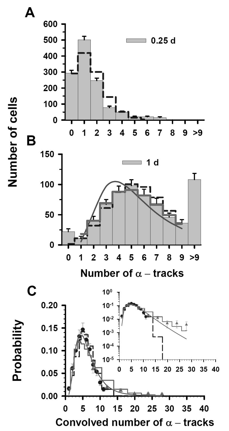
Statistical analysis of α-particle track distribution in V79 lung fibroblasts that were labeled in culture medium containing 67 kBq/mL ²¹⁰Po-citrate. Decays were allowed to accumulate for 0.25 d (A) and 1 d (B). The data points in Panel C represent a normalized convolution of the experimental track data obtained at 0.25 d (▲) and 1 d (●). Error bars, dashed step line, thick solid step line, solid curve and the inset are all as explained in Fig. 1. The parameters of the three probability density functions are also enumerated in Table 1.

DISCUSSION

As described above, a variety of approaches were used to analyze our ²¹⁰Po alpha particle track distribution data. These involve statistical analyses of both the raw track data and the convolved track data using P, LN, and P-LN functions. The results, summarized in Table 1, indicate that the P distribution alone does not adequately describe the observed track distributions as it would if the cellular activity was distributed equally among all the cells in the population. In fact, with the exception of the data corresponding to the highest concentration of ²¹⁰Po, a pure LN distribution generally provides the best description of the data. In the case of the highest concentration (67 kBq/mL), the data are best described by the P-LN distribution which suggests that the Poisson statistics associated with radioactive decay plays a significant role in the analysis of this set of autoradiographic data. Nevertheless, the underlying distribution of activity in this cell population is well described by a LN distribution.

It is interesting to more closely examine the conditions under which Poisson statistics play a significant role in interpreting our alpha particle track data. Figures 1C, 2B, and 3B show that the autoradiographic track data appear become more Poissonian as the concentration of ²¹⁰Po-citrate in the culture medium is increased. This is supported by the χ̂² values for the Poisson, LN and P – LN distributions. Notably, for the 1 d data set (67 kBq/mL), the corresponding values are 1.1, 5.6 and 0.66, respectively (Table 1). The reason for the increased Poisson influence at higher concentrations of ²¹⁰Po-citrate may be related to a decrease in the time interval for the observation (i.e. short emulsion exposure time). However, the χ̂² values for Poisson fits to the very short time interval 0.25 d data set (67 kBq/mL) and the 0.67 d data set (3.8 kBq/mL) are 91 and 96 (data are not shown in Table 1). These high values are indicative of a poor fit which suggests that the time interval may not be a significant factor.

It is also possible that the Poisson distribution plays a bigger role with increasing concentration of ²¹⁰Po-citrate because of a reduction in nonuniformity in the distribution of radioactivity among the cell population. To further pursue this possibility, the value of the log normal shape parameters (σ) obtained by the various methods described above are graphically compared in Fig. 4. The dashed line connects what we believe are the best values for σ, where best is defined as the lowest χ̂² (Table 1). Based on the linearity of the three data points on a logarithmic scale, the shape parameter is exponentially dependent on the extracellular concentration. A decreasing value of σ implies more uniform distribution of radioactivity among the cell population. This implies that the nonuniformity of the cellular uptake of ²¹⁰Po-citrate decreases with increasing extracellular concentration (7,8). Figure 6 in Ref. (7) shows that this will result in a more exponential survival curve rather than the saturating dose response curves that are expected for log normal distributions with large σ values.

Figure 4.

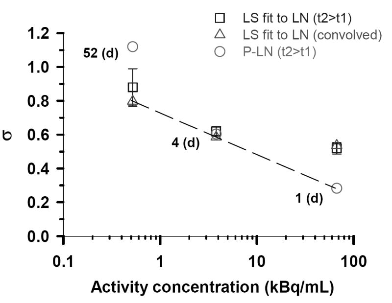
Log normal shape parameters (σ) for the three different activity concentrations of ²¹⁰Po-citrate. The open squares (□) represent the values of σ obtained, when <n> was constrained, by least squares fits of the experimental track data corresponding to the longest decay accumulation times (i.e. t₂>t₁, Figs. 1C, 2B, 3B) to a LN distribution function. Standard errors of these fitted σ values are indicated by the vertical lines. The corresponding σ values obtained for these same data using the P–LN distribution function are shown as open circles (○). The open triangles (△) correspond to least squares fits of the convolved data (Figs. 1D, 2C, 3C) to the LN function. Finally, the dashed line passes through what are considered the best σ values as defined by the lowest χ̂².

In our earlier article we used the convolution approach to analyze the experimental alpha particle track data (7). Kvinnsland et al. expressed concern regarding the convolution approach in relation to the impact of Poisson statistics on the resulting distribution (9). It is worth emphasizing again here that the overlapping regions of convolved data from independent data sets (Figs. 1D, 2C, 3C) suggest that the data can be convolved. The shape parameters obtained by LS fit of the primary data set (1-9 tracks, t₂ > t₁) and the convolved data to a LN function are also similar for the 0.52 and 3.8 kBq/mL cases which also supports the convolution approach. However, as shown in Fig. 4, the convolution approach is not satisfactory for the 67 kBq/mL data sets. In this case, as described above, the underlying LN distribution must be extracted from the measured distribution using the P-LN function. Thus, caution must be exercised when implementing the convolution approach. With this in mind, it should also be noted that the σ values obtained directly from the 52 d data and the 4 d data are very similar to those obtained from the convolved data. Therefore, provided that one has a single autoradiograph that covers most of the track distribution (e.g. Figs. 1C or 2B), one may be able to obtain σ without resorting to convolution.

In order to test the potential use of LN distributions to describe the cellular uptake of other radiochemicals within a population of cells, the data of Lehman et al. are revisited (18). Their cells were labeled with ³³P, an emitter of beta particles with a mean energy of 76.9 keV, under unstirred and stirred conditions, and the frequency distribution of autoradiographic grains per cell was measured. The authors noted that the distribution of background grains per cell was adequately described by a Poisson distribution, but the experimental treatments (stirred and unstirred mixtures) were not explained by a simple Poisson distribution. Consequently, they employed a Neyman’s Type A distribution which consists of a composite of two Poisson processes, one that describes grain counting statistics and the other process pertains to the randomness of radioactive decay (19). They fit their data to this distribution and obtained χ̂² values of 0.68 and 1.7 for the stirred and unstirred conditions, respectively. To assess the capacity of the LN distribution to describe their data, the arithmetic mean (<n>) was calculated for each mixture and a χ̂² analysis was conducted for Poisson, LN, P – LN. Furthermore, an unconstrained least squares fit of the data to a LN function was performed. The results of these fits show that the LN, P-LN, and LS fit to LN generally yield similar values of χ̂² and log normal shape parameters (Table 2). Thus, the underlying distribution of radioactivity among the cell population is well described by a log normal distribution.

TABLE 2.

The relevant parameters for the β–particle tracks per cell in a track autoradiography experiment (18) by employing the Poisson, LN and P – LN functions along with the quantities of statistical tests (χ̂² and/or R²) for the stirred and unstirred mixture.

Type	Predicted function	<n> ‡	σ§	v	χ̂2	R2
Stirred mixture	Poisson	8.7	—	22	0.15	—
	LN	8.7	0.70	20	0.0071	—
	P – LN	8.7	0.80	20	0.0064	—
	LS fit to LN	12 ± 1.4	0.79 ± 0.075	20	0.0048	0.79
Unstirred mixture	Poisson	7.8	—	21	0.99	—
	LN	7.8	0.67	20	0.0077	—
	P – LN	7.8	0.68	20	0.0046	—
	LS fit to LN	8.2 ± 0.37	0.57 ± 0.033	20	0.018	0.93

The value of arithmetic mean (<n>) and the shape parameter (σ) are obtained from the raw data of (18) and the minimization of χ̂² value, respectively.

^{‡, §}and the Standard Errors are as described in Table 1.

The analyses above support the conclusion that the distribution of radioactivity in a cell population can often be well represented by a LN distribution. Log normal distributions have been shown to describe a variety of natural processes. Bulmer (20) fitted the species abundance data which showed truncated, grouped LN distributions provided a satisfactory fit over the logarithmic and P – LN models, omitting zero class. There are also other models that can be useful for explaining data with a priori knowledge of the underlying distribution, such as multivariate P – LN distributions (21), bivariate Poisson distributions (19), etc. However, log normal distributions are ubiquitous and have been observed across many fields (22,23).

Finally, this exercise was undertaken to demonstrate the statistical significance of the log normal distribution that was obtained for ²¹⁰Po-citrate using an alpha particle track autoradiographic approach (7). The reliability of this approach stems from its use of emitted radiations to ascertain the distribution. Other experimental techniques, such as flow cytometry (24,25), can also be used to derive the distribution. Because of the ubiquitous presence of LN distributions, many investigators studying radiobiological responses to radiopharmaceuticals and other radiochemicals may find this distribution useful to fold into their dose response models (8,24,26). Its implementation is facilitated by a number of factors. First, and foremost, it is an analytical function that is described by only two parameters (σ, μ). Second, the LN probability density function is provided in standard subroutine libraries (e.g. National Algorithm Group (NAG)) for computational purposes.

CONCLUSIONS

Statistical tests show that the log normal distribution function is favored as a general form to describe the distribution of cellular uptake of ²¹⁰Po among a population of cells exposed to the same concentration of ²¹⁰Po-citrate. Furthermore, there is evidence to suggest that this distribution is likely to be applicable to a variety of radiopharmaceuticals.

References

- 1.Leblond CP, Wilkinson GW, Belanger LF, Robichon J. Radio-autographic visulization of bone formation in the rat. The Journal of NIH Research. 1997;9:44–55. doi: 10.1002/aja.1000860205. [DOI] [PubMed] [Google Scholar]
- 2.Soremark R, Hunt VR. Autoradiographic studies of the distribution of polonium-210 in mice after a single intravenous injection. Int J Rad Biol. 1966;11:43. doi: 10.1080/09553006614550781. [DOI] [PubMed] [Google Scholar]
- 3.Jönsson B-A, Strand S-E, Larsson BS. A quantitative autoradiographic study of the heterogeneous activity distribution of different indium-111-labeled radiopharmaceuticals in rat tissues. J Nucl Med. 1992;33:1825–1832. [PubMed] [Google Scholar]
- 4.Roberson PL. Quantitative autoradiography for the study of radiopharmaceutical uptake and dose heterogeneity. J Nucl Med. 1992;33:1833–1835. [PubMed] [Google Scholar]
- 5.Humm JL, Macklis RM, Bump K, Cobb LM, Chin LM. Internal dosimetry using data derived from autoradiographs. J Nucl Med. 1993;34:1811–1817. [PubMed] [Google Scholar]
- 6.Akabani G, Kennel SJ, Zalutsky MR. Microdosimetric analysis of alpha-particle-emitting targeted radiotherapeutics using histological images. J Nucl Med. 2003;44:792–805. [PubMed] [Google Scholar]
- 7.Neti PVSV, Howell RW. Log normally distributed cellular uptake of radioactivity: Implications for biological responses to radiopharmaceuticals. J Nucl Med. 2006;47:1049–1058. [PMC free article] [PubMed] [Google Scholar]
- 8.Neti PVSV, Howell RW. Biological response to nonuniform distributions of 210Po in multicellular clusters. Radiat Res. 2007;168:332–340. doi: 10.1667/RR0902.1. [DOI] [PMC free article] [PubMed] [Google Scholar]
- 9.Kvinnsland Y, Stokke T, Aurlien E. Log normal distribution of cellular uptake of radioactivity. J Nucl Med. 2007;48:327. author reply 327-328. [PubMed] [Google Scholar]
- 10.Neti PV, Howell RW. Reply: log normal distribution of cellular uptake of radioactivity. J Nucl Med. 2007;48:327a–328. [PMC free article] [PubMed] [Google Scholar]
- 11.Handel PH. Quantum approach to 1/f noise. Phys Rev A. 1980;22:745–757. [Google Scholar]
- 12.Kousik GS, Gong J, Van Vliet CM, et al. Flicker noise fluctuations in α-radioactive decay. Can J Phys. 1987;65:365–375. [Google Scholar]
- 13.Azhar MA, Gopala K. Search for 1/f fluctuations in α decay of 210Po. Phys Rev A. 1989;39:5311–5313. doi: 10.1103/physreva.39.5311. [DOI] [PubMed] [Google Scholar]
- 14.Miller G. Statistical modelling of Poisson/Log-normal data. Radiat Prot Dosimetry. 2007 doi: 10.1093/rpd/ncl544. [DOI] [PubMed] [Google Scholar]
- 15.Aitchison J, Brown JAC. The Log-normal Distribution. Cambridge: Cambridge University Press; 1957. [Google Scholar]
- 16.Crow EL, Shimizu K. Lognormal distributions: theory and applications. New York: Marcel Dekker; 1988. [Google Scholar]
- 17.Fors O, Núñez J, Richichi A. CCD drift-scan imaging lunar occultations: A feasible approach for sub-meter class telescopes. Astronomy & Astrophysics. 2001;378:1100–1106. [Google Scholar]
- 18.Lehman JT, Scavia D. Microscale nutrient patches produced by zooplankton. Proc Natl Acad Sci U S A. 1982;79:5001–5005. doi: 10.1073/pnas.79.16.5001. [DOI] [PMC free article] [PubMed] [Google Scholar]
- 19.Johnson NL, Kotz S. Discrete distributions. Boston: Houghton-Mifflin; 1969. [Google Scholar]
- 20.Bulmer MG. On fitting the Poisson lognormal distribution to species-abundance data. Biometrics. 1974;30:101–110. [Google Scholar]
- 21.Aitchison J, Ho CH. The multivariate Poisson-log normal distribution. Biometrika. 1989;76:643–653. [Google Scholar]
- 22.Mitzenmacher M. A brief history of generative models for power law and lognormal distributions. Internet Mathematics. 2004;1:226–251. [Google Scholar]
- 23.Limpert E, Stahel WA, Abbt M. Log-normal distributions across the sciences: keys and clues. Bioscience. 2001;51:341–352. [Google Scholar]
- 24.Kvinnsland Y, Stokke T, Aurlien E. Radioimmunotherapy with alpha-particle emitters: microdosimetry of cells with a heterogeneous antigen expression and with various diameters of cells and nuclei. Radiat Res. 2001;155:288–296. doi: 10.1667/0033-7587(2001)155[0288:rwapem]2.0.co;2. [DOI] [PubMed] [Google Scholar]
- 25.Pinto M, Howell RW. Concomitant quantification of targeted drug delivery and biological response in individual cells. Biotechniques. 2007;43:64, 66–71. doi: 10.2144/000112492. [DOI] [PMC free article] [PubMed] [Google Scholar]
- 26.Ballangrud AM, Yang WH, Palm S, et al. Alpha-particle emitting atomic generator (Actinium-225)-labeled trastuzumab (herceptin) targeting of breast cancer spheroids: efficacy versus HER2/neu expression. Clin Cancer Res. 2004;10:4489–4497. doi: 10.1158/1078-0432.CCR-03-0800. [DOI] [PubMed] [Google Scholar]