Gene-set analysis and reduction

Abstract

Gene-set analysis aims to identify differentially expressed gene sets (pathways) by a phenotype in DNA microarray studies. We review here important methodological aspects of gene-set analysis and illustrate them with varying performance of several methods proposed in the literature. We emphasize the importance of distinguishing between ‘self-contained’ versus ‘competitive’ methods, following Goeman and Bühlmann. We also discuss reducing a gene set to its subset, consisting of ‘core members’ that chiefly contribute to the statistical significance of the differential expression of the initial gene set by phenotype. Significance analysis of microarray for gene-set reduction (SAM-GSR) can be used for an analytical reduction of gene sets to their core subsets. We apply SAM-GSR on a microarray dataset for identifying biological gene sets (pathways) whose gene expressions are associated with p53 mutation in cancer cell lines. Codes to implement SAM-GSR in the statistical package R can be downloaded from http://www.ualberta.ca/~yyasui/homepage.html.

GENE-SET ANALYSIS METHODS

Increasing use of DNA microarrays in biomedical research has been stimulating methodological research on data-analytical approaches that help gain insights into biological functions of genes and pathways. One important goal of microarray data analyses is to evaluate the association of a priori defined gene sets with a phenotype of interest, i.e. gene-set analysis. Using gene sets, often taken from databases, such as Gene Ontology, KEGG and BioCarta, many gene-set analysis methods follow a two-step algorithm:

Gene-set analysis algorithm

1. A test statistic that is intended to measure the deviation of gene-set expression measurements from the null hypothesis of no association with the phenotype is calculated.

2. Statistical significance (P-value) for each gene set is calculated based on permutations of samples.

When there are a large number of gene sets being evaluated, the statistical significance for each gene set is often corrected for multiple testing of many hypotheses (gene sets) [1] or a false discovery rate [2] of each gene set is calculated instead.

The gene-set analysis methods vary by the test statistic used in (1). In their review paper, Nam and Kim [3] lists gene-set analysis methods, availability and reference in Tables 1 and 2, as well as gene-set databases for various organisms in Table 3. We give here details on several gene-set analysis methods, including their capability to handle various phenotypes. Gene-set enrichment analysis (GSEA), proposed by Mootha et al. [4] and improved by Subramanian et al. [5], for example, uses an enrichment score based on a Kolmogorov–Smirnov statistic as the test statistic. GSEA is currently the most popular method for gene-set analysis, with a user-friendly desktop application, which can be downloaded from www.broad.mit.edu/gsea. An extensive collection of gene sets and pathways are also available from the same website. Significance analysis of function and expression (SAFE) proposed by Barry et al. [6] extends GSEA to cover multiclass, continuous and survival phenotypes, and gives analysts more options for the test statistic: Wilcoxon rank sum; Kolmogorov–Smirnov and Hypergeometric statistic. SAFE is available as an R package in Bioconductor: http://bioconductor.org/packages/2.0/bioc/html/safe.html. Jiang and Gentleman [7] extend GSEA to allow for covariates adjustments and discuss the use of principal component analysis to reduce the gene sets prior to the enrichment analysis. Goeman et al. [8] employed a score test based on a random-effect logistic model fit for each gene set, and subsequently extended their method to multiclass, continuous and survival phenotypes, and allowed for covariate adjustments [9]. Their method is available as an R package called GlobalTest: http://bioconductor.org/packages/2.0/bioc/html/globaltest.html. Mansmann and Meister [10] used an analysis of covariance (ANCOVA) F-test to measure the deviation of gene sets from the null hypothesis, and their method accommodating multiclass, continuous phenotypes and covariate adjustments, is available as an R package in Bioconductor: http://bioconductor.org/packages/2.2/bioc/html/GlobalAncova.html. To account for the multivariate structure of the gene sets, Kong et al. [11] uses Hotelling's T² and either the original data or an orthonormal projection, depending if the dimensionality assumption for the multivariate test holds or not. Dinu et al. [12] pointed out critical problems of GSEA and extended a single-gene analysis by significance analysis of microarray (SAM) [13] to gene-set analysis (SAM-GS). Their test statistic was the L₂ norm of the vector of the SAM statistics, corresponding to the genes in the gene set of interest. The use of the SAM statistic accounted for the small variability of a subset of genes, a characteristic feature of microarray data [13]. SAM-GS software is available in Excel, Python and R (www.ualberta.ca/~yyasui/homepage.html). In line with the work of Dinu et al. [12] and Goeman et al. [8, 9], Adewale et al. [14] proposed a unified gene-set analysis approach of diverse phenotypes, including multi-class, continuous and censored-survival phenotypes, while allowing covariate adjustments and correlated phenotypes by use of regression methods. Implementations for various phenotypes are available in R.

Table 1:

P-values for the three ‘self-contained null hypothesis’ and three ‘competitive null hypothesis’ approaches for the genes sets with P-value ≤ 0.001 by any of the six methods

p53 link	Gene set	Self-contained null hypothesis						Competitive null hypothesis
		Before standardization			After standardization
		Global	ANCOVA	SAM-GS	Global	ANCOVA	SAM-GS	SAFEa	GSEAa	Fishera
Pathway member	ATM pathway	<0.001	<0.001	<0.001	<0.001	0.002	<0.001	0.494	0.215	0.984
	p53 signaling pathway	0.112	0.101	<0.001	0.003	0.003	0.001	0.289	0.013	0.994
	p53_UP	0.003	0.004	<0.001	<0.001	<0.001	<0.001	0.413	<0.001	1.000
	p53hypoxia pathway	0.626	0.622	<0.001	<0.001	<0.001	<0.001	0.343	<0.001	1.000
	p53 pathway	0.142	0.150	<0.001	<0.001	<0.001	<0.001	0.273	<0.001	1.000
	Radiation_sensitivity	0.119	0.135	<0.001	<0.001	<0.001	<0.001	0.204	0.002	0.998
	CR_DEATH	0.001	0.004	0.008	0.029	0.017	0.004	0.718	0.314	0.833
Apoptosis	BAD pathway	<0.001	0.007	<0.001	<0.001	<0.001	<0.001	0.029	0.044	0.996
	Hsp27pathway	0.047	0.044	<0.001	<0.001	0.001	<0.001	0.027	<0.001	1.000
	Mitochondria pathway	0.002	0.002	<0.001	0.007	0.007	<0.001	0.543	0.329	0.923
	bcl2family & reg. network	0.102	0.100	0.001	0.001	0.005	<0.001	0.064	0.426	0.880
	Ceramide Pathway	0.002	0.006	0.001	0.004	0.004	<0.001	0.421	0.308	0.891
p53-induced proline oxidase mediates apoptosis via a calcineurin-dependent pathway	Calcineurin pathway	0.068	0.084	<0.001	0.007	0.002	<0.001	0.668	0.138	0.933
Cell cycle	Cell cycle regulator	0.021	0.017	<0.001	0.002	0.001	<0.001	0.025	0.293	0.969
	Raccycd pathway	0.177	0.181	<0.001	0.001	<0.001	<0.001	0.117	0.565	0.891
Integrated negative feedback loop between Akt and p53	SA_TRKA_RECEPTOR	0.254	0.252	<0.001	0.001	<0.001	<0.001	0.362	0.347	0.792
NA	HUMAN_CD34 _ ENRICHED_TF_ JP	0.584	0.566	0.699	0.734	0.721	0.471	0.989	0.3703	0.001

^aThe only additional gene set identified with P <0.001 by any of SAFE, GSEA and Fisher was HUMAN_CD34_ENRICHED_TF_ JP. For this gene set, Fisher P-value was <0.001, but all the other five methods gave P-values >0.37.

Table 2:

Extracting core subsets for p53 cell-lines

Gene set	Gene-set size	Core pathway size	Percent reduction	Core pathway members (SAM-GS P-values)
ATM Pathway	19	2	89.5	CDKN1A (0.001), MDM2 (0.001)
BAD Pathway	21	2	90.5	BAX (0.001), BCL2 (0.001)
bcl2family & reg. network	23	1	95.7	BAX (0.001)
Calcineurin pathway	18	1	94.4	CDKN1A (0.001)
Cell cycle regulator	23	2	91.3	CDKN1A (0.001), BTG2(0.002)
D _DAMAGE_SIG_LLING	90	5	94.4	CDKN1A (0.001), BAX (0.001), DDB2 (0.001), MDM2 (0.001), BTG2 (0.003)
drug_resistance_and_metabolism	95	2	97.9	CDKN1A (0.001), BAX (0.001)
g2 pathway	23	2	91.3	CDKN1A (0.001), MDM2 (0.001)
hsp27 pathway	15	4	73.3	FAS (0.001), TNFRSF6 (0.001), BCL2 (0.002), IL1A (0.002)
p53 signaling	87	3	96.6	CDKN1A (0.001), BAX (0.001), MDM2 (0.001)
p53hypoxia pathway	20	3	85.0	CDKN1A (0.001), BAX (0.001), MDM2(0.001)
p53 Pathway	16	3	81.3	CDKN1A (0.001), BAX (0.001), MDM2 (0.001)
Raccycd pathway	22	1	95.5	CDKN1A (0.001)
radiation_sensitivity	26	3	88.5	CDKN1A (0.001), BAX (0.001), MDM2 (0.001)
SA_TRKA_RECEPTOR	16	1	93.8	CDKN1A (0.001)
P53_UP	40	5	87.5	CDKN1A (0.001), BAX (0.001), DDB2 (0.001), MDM2 (0.001), BTG2 (0.003)
breast_cancer_estrogen_sig lling	97	3	96.9	CDKN1A (0.001), TNFRSF6 (0.001), ESR2 (0.003)
Ceramide pathway	22	1	95.5	BAX (0.001)
CR_DEATH	70	1	98.6	BAX (0.001)
Mitochondria pathway	19	1	94.7	BAX (0.001)
g1 pathway	26	1	96.2	CDKN1A (0.001)
SIG_IL4RECEPTOR_IN_B_LYPHOCYTES	26	1	96.2	STAT6 (0.001)
ST_Interleukin_4_Pathway	24	1	95.8	STAT6 (0.001)
ets pathway	16	2	87.5	SIN3B (0.003), CSF1R (0.004)
ca_nf_at_sig lling	95	2	97.9	CDKN1A (0.001), BCL2 (0.002)
cell_cycle_arrest	30	1	96.7	CDKN1A (0.001)
Cellcycle pathway	23	1	95.7	CDKN1A (0.001)
Chemical pathway	21	1	95.2	BAX (0.001)
ST_Fas_Sig ling_Pathway	56	1	98.2	BAX (0.001)
Cytokine pathway	21	2	90.5	IL1A (0.002), IFNA1(0.005)
Hivnef pathway	54	2	96.3	MDM2 (0.001), TNFRSF6 (0.001)

Core subsets extracted by SAM-GSR, for 31 sets significant at 0.01, using a cutoff c = 0.1 for c_k values.

In addition to the several examples listed above, many gene-set analysis methods have been proposed. Tian et al. [15] emphasized the importance of distinguishing between the gene-sampling versus subject-sampling methods. In an extensive review, Goeman and Bühlmann [16] Discussed methodological principles behind gene-set analysis and established the distinction between testing ‘self-contained null hypotheses’ that use subjects/specimens as the sampling units and testing ‘competitive null hypotheses’ that use genes as the sampling units. The former evaluates self-contained null hypothesis in the sense that the test statistic requires only the gene expression measurements of the gene set being tested. The latter evaluates competitive null hypothesis in the sense that the test statistic compares the gene expression measurements of the gene set being tested to those of the genes outside of this set. Goeman and Bühlmann [16] strongly recommended against the testing of competitive null hypotheses with the use of gene-sampling methods, on the grounds of its untenable statistical independence assumption across genes. Delongchamp et al. [17] also commented on how ignoring the correlations within the sets can overstate significance, and propose meta-analysis methods for combining P-values with a modification to adjust for correlation. In their review paper, Nam and Kim [3] revisited the two different null hypotheses for testing the association of a gene set with a phenotype, as introduced by Tian et al. [15]. The first type of hypothesis, called Q1, is competitive and tests whether the level of association of a gene set with the phenotype is equal to those of the other gene sets. The second type of hypothesis, called Q2, is self-contained and tests whether gene expressions of a gene set differ by the phenotype. They ran a simulation study and compare the performance of competitive, self-contained and GSEA methods. We would like to emphasize that the data used by Nam and Kim [3] simulation study was generated under Q1, and therefore it is expected that competitive methods would return a uniform P-value, and self-contained methods would identify most of the sets as being differentially expressed. In their simulation study, 30% of all genes were truly differentially expressed and each gene set was built such that 30% of genes in each gene set are differentially expressed. The competitive-methods community thinks that no gene set generated according to this simulation scheme should be called differentially expressed because all gene sets have the same level of association with the phenotype. On the other hand, the self-contained-methods community thinks that all genes sets should be called differentially expressed because 30% of genes of each gene set are differentially expressed. This fundamental disagreement on the concept of, not the methods for identifying, differentially expressed gene sets has not been recognized in the literature, and it is a key point in the debate between the self-contained versus competitive methods.

To further illustrate this disagreement, we performed a simulation study based on Q2, and showed that it is supportive of self-contained methods over competitive ones. This study compared the distribution of P-values obtained from the analyses of the three hypotheses Q1, Q2 and Q3 on simulated data. We generated expression profiles of 4000 genes with two groups, each having 20 samples. The first 2000 genes were divided into 100 gene sets, each of which contained 20 genes. The expression values in each of the 100 sets followed a multivariate normal distribution, with mean vector zero, and variance–covariance matrix with constant off-diagonal entry generated from Unif (0.5, 0.9) (i.e. no gene was differentially expressed between the two groups, and pairs of genes within each set have a constant correlation generated uniformly from 0.5 to 0.9). The expression values for the remaining 2000 genes were sampled from a standard normal distribution in both groups (i.e. no gene was differentially expressed between the two groups and the gene expression values are uncorrelated). Similar to the simulation study of Nam and Kim [3], we compared the difference of the three hypotheses using the average t-statistic in a gene set as the test statistic. Since none of the genes were differentially expressed, no gene sets were expected to be identified as significant. Indeed, the self-contained method (Q2) recognized no differentially expressed sets so the P-values were distributed uniformly (Figure 1). However, the competitive method (Q1) detected 27 of the 100 sets as differentially expressed with a P-value cutoff of 0.05. The mixed approach, GSEA, identified 64 of the sets as differentially expressed, which is a consequence of the fact that GSEA tests clustering of the genes in the correlation order, and this aspect has also been illustrated and explained by Dinu et al. [12]. Also, we would like to mention that when the set size was increased to 100 with a constant correlation of 0.9 within each set, competitive method identified 40 of the sets as being significant. This illustrates the wrong use of the gene sampling technique in situations where gene expressions within a set exhibit large correlations, a situation not uncommon in gene-set analysis of microarray data. Chen et al. [18] also argue their preference for Q2 over Q1, because the P-values computed under Q2 are consistent with the principle of statistical significance testing, while the P-values computed under Q1 do not take into account correlations among genes.

Figure 1:

The P-value distributions of 100 gene sets for the three GSA approaches on simulated data. A total of 10 000 permutations were performed for gene or sample randomizations on the average t-score.

Based on the simulation study, Nam and Kim [3] recommended the use of GSEA, because it is a mixed approach and its performance is in between the competitive and self-contained methods. We disagree that GSEA can be considered a mixed approach or that its performance is in between competitive and self-contained (Figure 1). Dinu et al. [12] showed how GSEA calls gene sets with genes clustered in the low correlation region as significant. GSEA is testing the ‘clustering’ of the gene-set's genes in the degree of association with a phenotype. Gene-set analysts would like to find gene sets that cluster at the high degree of association with the phenotype: these gene sets are truly differentially expressed. But GSEA will find gene sets whose genes cluster at any degree of association, including no association. This tendency for leading to false positive findings is one major problem of GSEA. Also, GSEA has a tendency for leading to false negative findings if differentially expressed gene sets have genes whose degrees of association with the phenotype are heterogeneous (i.e. a mix of differentially expressed genes and not differentially expressed genes). The testing of clustering is not going to pick up gene sets that have mixed degrees of association (i.e. not all genes are clustered).

Another aspect we would like to comment on is that Nam and Kim [3] recommends using all methods simultaneously, if possible, with biological analyses. We agree that it is useful to compare different methods, as long as the user is aware of their advantages and limitations.

Care must be exercised when conducting simulation studies to compare self-contained and competitive methods. Any simulation study based on data generated under either Q1 or Q2 would be naturally supportive of competitive or self-contained methods, respectively. We agree about a concern on the self-contained methods that a small number of genes in the gene set can make the set significantly differentially expressed. In this situation, we recommend the use of gene-set reduction to a core subset that can be further interpreted by the scientist. We present an approach to gene-set reduction, and illustrate its use on a real data set, in the next two sections.

Although a large number of gene-set analysis methods have been proposed, little attention has been paid to comparative performances of the various methods. Liu et al. [19] compared the performance of three ‘self-contained null hypothesis’ testing methods, global test [9], ANCOVA global test [10] and SAM-GS [12], via simulated and real-world microarray data analyses, both statistically and biologically. They found that global test and ANCOVA global test require an appropriate standardization of gene expression measurements across genes for proper performance. After standardization of these two methods, the performance of all three methods was very similar, when using permutation-based inference, with a slight power advantage in SAM-GS (Table 1). Liu et al. [19] also applied three ‘competitive null hypothesis’ testing methods in the real data comparisons: GSEA [5]; SAFE [6] and Fisher's exact test [20]. Note that, while Fisher's exact test is truly a ‘competitive’ method, GSEA and SAFE are hybrids between ‘self-contained’ and ‘competitive’ approaches: their test statistic is motivated by a gene-sampling model of ‘competitive’ methods, whereas a subject-sampling model of ‘self-contained’ methods is used for calculating statistical significance of phenotype-associated differential gene expression of each gene set [19]. Liu et al. [19] showed clearly diverging results between ‘self-contained’ and’competitive’ methods. These results, summarized in Table 1, show low power of the ‘competitive’ methods for identifying differential expression by phenotype of gene sets that are known to have biological links to p53. To exemplify, the ‘self-contained’ methods identified as differentially expressed all the seven gene sets containing p53 as a member, whereas SAFE and Fisher's exact test missed on all these sets and GSEA missed on two of the seven sets. The five gene sets involved in apoptosis were identified by the ‘self-contained’ methods, whereas SAFE and GSEA missed on three of them, and Fisher's exact test did not identify any of them. To summarize, the ‘self-contained’ methods (two global tests and SAM-GS) identified properly the gene sets with biological links to p53 as significant, whereas the ‘competitive’ methods missed on an appreciable proportion of these sets. These findings are in line with the methodological discussions offered by Goemann and Bühlmann [16] in their review paper. Goemann and Bühlmann [16] state that they expect these differences in performance between the two types of methods to be more evident when dealing with datasets where a large number of genes are differentially expressed.

Gene-set reduction

Gene-set analysis considers gene sets and pathways that are fixed a priori, typically from databases such as Gene Ontology, KEGG and BioCarta. In many applications, this meets the central goal of microarray data analyses. In other applications, however, gene sets are not well-established a priori and scientific interest may focus on the membership of gene sets based on the information provided in the microarray data being analyzed. Suppose, for example, there was a preliminary in-house gene set that was a priori assembled and hypothesized by a research team for its differential gene expression by the phenotype of interest. If a gene-set analysis identifies differential expression of this gene set in the microarray data, a natural next step would be to ask: ‘are all members of this gene set essential, or is a subset sufficient, in considering its link with the phenotype of interest?’ We consider here a method for extracting a core set of genes that chiefly contribute to the statistical significance of differential expression of a given gene set by a phenotype. The method is referred to as SAM-GS reduction (SAM-GSR), an extension of our SAM-GS analysis [12] to the gene-set reduction problem. We discuss the performance of the proposed method using simulations. Results and their biological interpretations of a SAM-GSR analysis, applied to a microarray study for identifying differentially expressed biological pathways by p53 mutation in cancer cell lines, are presented. Code to implement SAM-GSR in the statistical package R can be downloaded from http://www.ualberta.ca/~yyasui/homepage.html.

For gene-set analysis, SAM-GS [12] combines the t-like statistics of individual genes into a measure of association of a gene set with the phenotype. For a gene set S, SAM-GS is the L₂ norm of the t-like statistics:

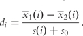
where d_i = x₁ (i) - x₂ (i) / s(i) + s₀ is calculated for each gene i, x₁ (i) and x₂ (i) are the sample averages corresponding to each of the two groups of the phenotype, s(i) is a pooled standard deviation over the two groups of the phenotype, and s₀ is a small positive constant that adjusts for the small variability in microarray measurements [12]. Statistical significance of S is obtained based on a phenotype-label permutation test.

Given a statistically significant association of the gene set S with the phenotype, we may consider a gene-set reduction analysis for S. We apply SAM-GS sequentially to subsets of the significant gene set S and identify a core set of genes that chiefly contribute to the statistical significance of S. In reducing the gene set S, we use the following principle: for a pair of genes in S, genes i and j, |d_i | > | d_j | suggests that gene j belongs to a subset only if gene i belongs to the subset. This principle is motivated by the fact that d_i² is the each gene's contribution to the test statistic SAM-GS and the core subset must consist of genes with larger contributions.

SAM-GSR gradually partitions the entire set S, into two subsets, based on the principle above and evaluates their association with the phenotype. SAM-GSR can be summarized in a few steps:

SAM-GSR Steps for a given gene set S:

(1) For each of the N genes, calculate the statistic d as in SAM for an individual-gene analysis as above:

(2) For k = 1, …, |S| − 1, select the first k genes with largest statistic |d| to form a reduced set R_k. Let R_k be the complement of R_k in S, and c_k be the SAM-GS P-value of R_k.

(3) The reduced set R_k corresponds to the least k such that c_k is larger than a threshold c, chosen by the analyst.

We note that by removing genes with joint statistical significance, as a set, above a threshold, i.e. c_k > c, we are protected against losing genes that are not significant by themselves, but collectively, they form a set that is significant. This gene-set scenario was discussed by GSEA developers, both [4] and [5], and it is not unusual in pathway analysis. Since SAM-GSR is based on joint statistical significance of subsets, it will tend to keep members of a set that are not significant by themselves, but as a set they become significant. The work on well-defined inferential criteria for gene selection, such as FDR, abounds and one can think of applying such criteria to extract core subsets, by simply using an FDR cutoff within the gene set, for example. However, we would like to point out that SAM-GSR selects core subsets by combining the contribution of each gene into an overall measure of association, rather than looking at individual FDR values. Also, an interesting aspect of pathway analysis is that by combining the genes into a measure of association, a tendency of multiple genes to work together towards the significance of the set is taken into account. A set consisting only of moderately associated genes can still be significant. SAM-GSR will tend to keep all members of such sets, because the subsets consisting of moderately associated genes can still be significant, while an individual FDR value criterion may be missing on moderately associated genes, and drop them from the set. This aspect will be exemplified in the next section.

We explain here the rationale behind selecting the core subsets based on c_k values rather than p_k values. We note that if a gene set is significantly associated with a phenotype, the reduced set will also be significant. Therefore, the p_k values can be really low in magnitude—we encountered the situation where they were all zero, even if R_k contains noise genes—making it difficult to choose a core pathway based on these values. On the other hand, the increasing trend in the c_k values, exhibited at the beginning of the reduction process, enables the user to choose from a range of cutoff values from more conservative such as 0.05 to more liberal such as 0.5, giving the user the flexibility to gradually include more genes in the core pathway.

We evaluated the performance of SAM-GSR in a simple simulation study as a proof-of-principle experiment. The results of the simulations are presented in the Appendix.

Extracting core subsets for p53 cancer cell-lines

To illustrate the application of SAM-GSR, we performed gene-set reduction analysis using a microarray dataset considered in Ref. [5], in which two types of cancer cell-lines were compared: 17 cell-lines with wild-type p53, and 33 cell-lines with mutant p53. Briefly, the microarray data were obtained by hybridizing mRNA to Affymetrix HGU95Av2 chip. These arrays contain 12 625 probe sets whose expressions were reduced from the probe level to the gene level of 10 100 unique genes, by taking the maximum probe set expression of each gene in each sample, as described in Ref. [5]. For gene sets, we used Subramanian et al.'s gene-set subcatalogs C2 from Ref. [5]. Catalog C2 consisted of 472 sets containing genes reported in manually curated databases, and 50 sets containing genes reported in various experimental papers. Following Ref. [5], we restricted the set size to be between 15 and 500, resulting in 308 gene sets.

SAM-GS analysis reveals 31 gene sets in the C2 catalog that are significantly associated with p53 wild-type versus mutant cancer cell-lines phenotype, at a cutoff P-value of 0.01, FDR of 0.033. We calculated the c_k values, k = 1, …, |S| − 1 for each of these sets. Intuitively, by gradually eliminating genes with large |d| statistic, the c_k values should increase, and this is confirmed throughout our results, see Figure 2 for an illustration using p53 signaling pathway. Table 2 shows the core subsets extracted by SAM-GSR, for these 31 sets, using a cutoff c = 0.1 for c_k values. On average, SAM-GSR reduced the number of genes in the 31 gene sets by 93%. Cyclin-dependent kinase inhibitor 1A, CDKN1A, a gene known to be regulated by p53 [21], appears most frequently in the 31 core subsets. Some well-characterized targets or regulators of p53 showing up in the core subsets include: BCL2-associated X protein (BAX) [22], B-cell leukemia/lymphoma 2 (BCL2) [22], MDM2 [23] and tumor necrosis factor receptor superfamily, member 6 (TNFRSF6) [24].

Figure 2:

Increasing trend of c_k, C_k,k = 1, …, |S| − 1, for p53 signaling. For k = 1, …, |S| − 1, we select first k genes with largest statistic |d| to form a reduced set R_k; c_k is the SAM-GS P-value of R_k, the complement of R_kin S.

We exemplify below the advantage of SAM-GSR over individual gene FDR cutoffs, for genes sets consisting of genes moderately correlated with the phenotype. One example of this sort is given by hsp27 Pathway: all the genes in this pathway exhibit moderate correlation with the phenotype, with individual FDR values ranging from 0.17 to 0.74. If we chose to reduce the set based on individual genes’ FDR values (cutoff 0.25, for example), we end up with a reduced set consisting of only two genes. It is unclear then if we kept all important genes in this way: in fact, the remaining genes actually formed a set with a fairly large SAM-GS statistic (P = 0.004). Other examples similar to this one are ets Pathway (individual gene FDR values ranging from 0.28 to 0.74) and cytokine Pathway (individual gene FDR values ranging from 0.30 to 0.74). We would like to point out that the FDR values are based on the total number of genes in the array, and therefore may be over-conservative when reported in the context of the selected sets, since these sets have been selected based on P-value cutoff 0.01, and FDR of 0.033. On the other hand, reporting the FDR values based on only the genes present in the selected sets, is not without problem, as it ignores the tens of thousands of genes tested across the array.

We encountered situations where a whole gene set is reduced to a single gene. That suggest the subset consisting of the remaining genes is not differentially expressed. If the significance of a set is due to only one gene, the set should be examined biologically with caution: for example, functional roles of the significant gene within the gene set may be considered subsequent to this finding.

To gain more insight into SAM-GSR behavior, we varied the cutoff c, incrementally from 0.05 to 0.5. Median FDR values, together with the inter-quartile range, from 25%-tile to 75%-tile were calculated for: (i) members of each core pathway, and (ii) members of the complement of the core pathway in the corresponding set. These summaries of FDR values of individual genes within the pathway, and also within its complement, were plotted for each cutoff value c, ranging from 0.05 to 0.5, in Supporting Text. There is a considerable separation between median FDR values corresponding to members of the core pathway and its complement. In addition, there is very little overlap between the FDR inter-quartile ranges of the core pathway and its complement. The median and inter-quartile ranges tend to get closer for larger cutoffs c as expected. These results are consistent throughout the 31 gene sets, indicating that SAM-GSR is useful in extracting core subsets.

DISCUSSION

We reviewed here some key issues associated with gene-set analysis methods, and emphasized the discrepancy between the two types of methods dividing the literature devoted to this topic: self-contained versus competitive methods. Gene-set analysts must know that, while a large number of gene-set analysis methods are available, their performances are greatly different and they do not lead to the same scientific conclusions. In particular, in a study of p53 wild-type versus mutant cancer cell-lines, the ‘competitive’ methods missed on many of the gene sets linked to p53, whereas the ‘self-contained’ methods identified these sets as important.

We also explore a new direction: gene-set reduction. Large gene sets may achieve statistical significance for their association with the phenotype, although not all members are essential: we illustrated here the use of SAM-GSR to reduce gene sets to smaller sets. We would like to emphasize that SAM-GSR does not change the list of significant genes. SAM-GSR is not testing any specific null hypothesis. It is simply a useful analytical tool to reduce a gene set that has previously been found differentially expressed, to a core set, by gradually exploring the association of remaining genes as a set with a phenotype. Its stopping rule (i.e. the cutoff value) is arbitrarily chosen by the analyst without any claimed statistical properties associated with a given specific choice. The analyst can choose the cutoff (possibly multiple cutoffs) conservatively or liberally and consider the reduced set(s) with respect to the whole set in biological terms. Using different cutoffs for different gene sets is possible for a more flexible reduction.

Reducing a significant gene sets to core subsets is a useful step towards understanding biological mechanisms underlying the gene-set association with the phenotype of interest: a smaller number of genes are easier to understand and facilitate biological insight into disease processes. Other arguments for gene set reduction are listed below. Reduction to the most predictive genes might allow for targeted therapies and intervention strategies [25]. Limiting the number of genes facilitates a change of platform from a high-throughput microarray technology to alternative methods, such as real-time PCR that are cheaper and quicker, increasing the applicability to routine clinical setting for diagnostic purposes [25–27]. If there are redundant genes, examination of their expression levels would not improve clinical decisions but increases unnecessary costs. Finally, validation studies for robustness, reliability, patenting and commercialization, implementation in different centers with different platforms are greatly facilitated by using core subsets.

Key Points.

• Review gene-set analysis methods.

• Give gene-set analysts practical guidance in choosing between the many methods.

• Emphasize the discrepancy between self-contained versus competitive methods.

• Explore a new direction: gene-set reduction using SAM-GSR.

• Illustrate the use of SAM-GSR in extracting core subsets, by taking a study of p53 wild-type versus mutant cancer cell-lines, together with biologically defined gene sets, as an example.

FUNDING

National Cancer Institute—the Seattle Colorectal Family Registry (grant CA074794 to J.D.P.); Genome Canada, Genome Alberta, Roche Molecular Systems, Hoffmann La-Roche Canada, University of Alberta Hospitals Foundation, Alberta Innovation and Science, Roche Organ Transplant Research Foundation, the Canadian Institutes of Health Research, Kidney Foundation of Canada, Roche Germany, Astellas Canada, and the Muttart Foundation (to Halloran Lab.); Canada Research Chair Program (to P.H. and Y.Y.); the Alberta Heritage Foundation for Medical Research (to I.D., A.J.A. and Y.Y.); Canadian Institute of Health Research (to Y.Y.).

Supplementary Data

Supplementary data are available online at http://bib.oxfordjournals.org/.

Biographies

Irina Dinu is an assistant professor in the School of Public Health, University of Alberta. She received her PhD in applied statistics from the University of Alberta. Dr Dinu's main research focus is to develop biostatistical tools for analysis of microarray data.

John D. Potter is Director of International Research, Public Health Sciences Division, Fred Hutchinson Cancer Research Center. He focuses on etiology and the prevention of colon cancer; gene environmental interactions and the etiology of cancer; and how plan foods lower risk of cancer.

Thomas Mueller is an assistant professor in the Department of Medicine, University of Alberta. Dr Mueller's; research focuses on lymphocyte depletion and immune reconstitution, immune monitoring and gene expression profiles in organ transplantation.

Qi Liu received her master degree in Statistics from the University of Alberta in 2005. She is a full-time research assistant in the School of Public Health, University of Alberta, focusing on childhood cancer survivor study and biomarker discovery study.

Adeniyi J. Adewale finished his PhD in Statistics at University of Alberta in 2006. His research interests include the development of biostatistical methods for design and analysis of microarray experiments, issues in robust design and analysis of experiments (in particular, clinical trials). In December 2007, he started to work as a Biometrician for Merck Research Laboratories (Merck & Co, Inc.).

Gian S Jhangri is an assistant professor in the School of Public Health. His research interests include occupational cancer case-control studies, survival analysis, design and analysis of clinical trials, and statistical/epidemiological methods.

Gunilla Einecke is currently completing a PhD program in the Department of Medical Microbiology and Immunology, University of Alberta. Her current focus of study is the regulation of gene expression in transplant kidneys undergoing rejection, and the use of Affymetrix microarrays to show how the pathology generated by an immunological process corresponds in its elements to the changes in the transcriptome.

Konrad S. Famulski received his PhD and DSc from the Nencki Institute of Experimental Biology at the Polish Academy of Sciences. As a research associate in the Department of Medicine, University of Alberta, he focuses on signal transduction, genomics and proteomics.

Philip Halloran is currently the Director of the Alberta Transplant Applied Genomics Centre and is a professor in the Departments of Medicine and Medical Microbiology & Immunology at the University of Alberta, and the recipient of a Canada Research Chair in Transplant Immunology. His recent interests have focused on the diagnostic applications of microarrays in organ transplantation.

Yutaka Yasui is a professor in the School of Public Health, University of Alberta, and the recipient of a Canada Research Chair in Biostatistics and Epidemiologic Methods. His research is focused on developing and applying biostatistical and epidemiologic methods in the intersection of biology and clinical/public health sciences, especially on quantitative issues in biomarker discovery research.

APPENDIX—GENE-SET REDUCTION SIMULATION EXPERIMENT

We evaluated the performance of SAM-GSR in a simple simulation study as a proof-of-principle experiment. We randomly generated gene expression levels for a gene set of size n, for a total of M subjects, M/2 in each of two phenotype groups. Out of the n genes, s were differentially expressed, and the remaining genes were from i.i.d. N(0,1) distribution. The s differentially expressed genes were generated from MVN(μ_i,∑) where μ_1,j = γ, and μ_2,j = 0, for j = 1, …, s, so that the difference between the two phenotype groups’ means is μ_1,j − μ_2,j = γ, and the s × s matrix ∑ was block-diagonal with two identical blocks whose diagonal and off-diagonal elements were 1 and 0.5, respectively. We checked if SAM-GSR selects core subsets consisting of the s differentially expressed genes.

In the simulation experiment, we generated sets of n = 10, 20, 60 and 100 genes, such that s of them were differentially expressed. We used a sample size of M = 40, with 20 subjects in each group. We varied the distance between means of the two phenotype groups, γ = 0, 1, 2 and 5, and also the number of differentially expressed genes s, were given as the percent of genes in the gene set that are differentially expressed: 0%, 5%, 10%, 50% and 100%. We checked if SAM-GSR selects core subsets consisting of the s differentially expressed genes. Table A1 shows the results in term of percent of genes selected by SAM-GSR in the reduced sets, corresponding to cutoffs c = 0.05, c = 0.1 and c = 0.2, averaged over 1000 iterations.

Table A1:

Performance of SAM-GSR

γ	Percent genes differentially expressed	c = 0.05				c = 0.1				c = 0.2
		Set size				Set size				Set size
		10	20	60	100	10	20	60	100	10	20	60	100
0	0	0.4(2)	0.3(1.4)	0.1(.5)	0.1(.3)	0.5(2.7)	0.4(1.8)	0.2(0.7)	0.1(0.5)	0.7(3.8)	0.5(2.5)	0.2(1.1)	0.2(0.8)
1	5	–	5.3(1.4)	2.5(1.3)	2.3(1.3)	–	5.5(2.2)	2.9(1.6)	2.8(1.5)	–	6.1(3.2)	3.7(2.1)	3.4(1.8)
	10	10.4(2.2)	6.3(2.5)	5.4(2.5)	5.6(2.3)	10.9(3.3)	7.1(3.2)	6.3(2.7)	6.3(2.3)	12.2(5.3)	8.6(4.3)	7.4(2.9)	7.3(2.5)
	50	36.6(10.8)	37.8(8.7)	39.6(7.3)	39.6(7.2)	40.5(10.6)	40.5(8.3)	41.6(6.6)	41.4(6.5)	45(10.4)	43.9(7.9)	43.7(6)	43.3(5.8)
	100	86(16.7)	86.9(15)	86.8(14.4)	88.1(13.7)	91.8(13.4)	91.5(12.4)	91.1(11.8)	92(10.9)	96.2(9.5)	95.4(9.5)	94.7(8.9)	95.3(7.9)
2	5	–	5.3(1.6)	4.8(0.9)	4.6(0.7)	–	5.6(2.3)	5(1)	4.8(0.8)	–	6.3(3.4)	5.4(1.3)	5.2(1)
	10	10.5(2.4)	10.1(1.4)	9.6(1)	9.5(0.9)	11(3.5)	10.5(1.9)	9.9(1.1)	9.8(1)	12.5(5.5)	11.3(2.9)	10.4(1.4)	10.2(1.2)
	50	50.4(2.4)	50.1(1.5)	49.6(1)	49.5(0.8)	51(3.4)	50.6(2)	50(1)	49.7(0.8)	52.5(5.2)	51.3(3)	50.4(1.3)	50.1(1)
	100	100(0)	100(0)	100(0)	100(0)	100(0)	100(0)	100(0)	100(0)	100(0)	100(0)	100(0)	100(0)
5	5	–	5.3(1.6)	5.1(0.5)	5.1(0.4)	–	5.6(2.3)	5.2(0.8)	5.2(0.6)	–	6.3(3.4)	5.5(1.2)	5.4(0.9)
	10	10.6(2.5)	10.3(1.2)	10.1(.5)	10.1(0.4)	11(3.6)	10.6(1.8)	10.2(0.8)	10.2(0.6)	12.7(5.5)	11.3(2.9)	10.5(1.2)	10.4(0.9)
	50	50.5(2.3)	50.2(1.2)	50.1(.5)	50.1(0.3)	51(3.4)	50.6(1.9)	50.2(0.7)	50.2(0.5)	52.2(5.2)	51.3(3)	50.5(1.1)	50.3(0.8)
	100	100(0)	100(0)	100(0)	100(0)	100(0)	100(0)	100(0)	100(0)	100(0)	100(0)	100(0)	100(0)

Percent of genes selected in the reduced set, for three cutoffs, c = 0.05, c = 0.1 and c = 0.2, averaged over 1000 iterations, together with standard errors. Sampling 5% does not apply for a set size as small as 10.

For cutoff c = 0.05 and 0.1, the percent of genes selected in the reduced set is close to the percent of genes differentially expressed, indicating that the performance of SAM-GSR is overall good, tending to improve with increased set size and γ, the mean expression difference between the two phenotype groups. SAM-GSR performance is poorer for the more liberal cutoff c = 0.2.

References

- Dudoit S, Shaffer JP, Boldrick JC. Multiple hypothesis testing in microarray experiments. Stat Sci. 2003;18(1):71–103. [Google Scholar]
- Benjamini Y, Hochberg Y. Controlling the false discovery rate: a practical and powerful approach to multiple testing. J R Stat Soc Ser B Methodol. 1995;57(1):289–300. [Google Scholar]
- Nam D, Kim SY. Gene-set approach for expression pattern analysis. Brief Bioinform. 2008;9:189–97. doi: 10.1093/bib/bbn001. [DOI] [PubMed] [Google Scholar]
- Mootha VK, Lindgren CM, Eriksson KF, et al. PGC-1alpha-responsive genes involved in oxidative phosphorylation are coordinately downregulated in human diabetes. Nat Genet. 2003;34:267–73. doi: 10.1038/ng1180. [DOI] [PubMed] [Google Scholar]
- Subramanian A, Tamayo P, Mootha VK, et al. Gene set enrichment analysis: a knowledge-based approach for interpreting genome-wide expression profiles. Proc Natl Acad Sci USA. 2005;102(43):15545–50. doi: 10.1073/pnas.0506580102. [DOI] [PMC free article] [PubMed] [Google Scholar]
- Barry WT, Nobel AB, Wright FA. Significance analysis of functional categories in gene expression studies: a structured permutation approach. Bioinformatics. 2005;21:1943–9. doi: 10.1093/bioinformatics/bti260. [DOI] [PubMed] [Google Scholar]
- Jiang, Z, Gentleman R. Extensions to gene set enrichment. Bioinformatics. 2007;23:306–13. doi: 10.1093/bioinformatics/btl599. [DOI] [PubMed] [Google Scholar]
- Goeman JJ, van de Geer SA, de Kort F, et al. A global test for groups of genes: testing association with a clinical outcome. Bioinformatics. 2004;20:93–9. doi: 10.1093/bioinformatics/btg382. [DOI] [PubMed] [Google Scholar]
- Goeman JJ, Oosting J, Cleton-Jansen AM, et al. Testing association of a pathway with survival using gene expression data. Bioinformatics. 2005;21:1950–7. doi: 10.1093/bioinformatics/bti267. [DOI] [PubMed] [Google Scholar]
- Mansmann U, Meister R. Testing differential gene expression in functional groups. Goeman's global test versus an ANCOVA approach. Methods Inf Med. 2005;44:449–53. [PubMed] [Google Scholar]
- Kong SW, Pu WT, Park PJ. A multivariate approach for integrating genome-wide expression data and biological knowledge. Bioinformatics. 2006;22:2373–80. doi: 10.1093/bioinformatics/btl401. [DOI] [PMC free article] [PubMed] [Google Scholar]
- Dinu I, Potter JD, Mueller T, et al. Improving gene set analysis of microarray data by SAM-GS. BMC Bioinformatics. 2007;8:242. doi: 10.1186/1471-2105-8-242. [DOI] [PMC free article] [PubMed] [Google Scholar]
- Tusher VG, Tibshirani R, Chu G. Significance analysis of microarrays applied to the ionizing radiation response. Proc Natl Acad Sci USA. 2001;98(9):5116–21. doi: 10.1073/pnas.091062498. [DOI] [PMC free article] [PubMed] [Google Scholar]
- Adewale AJ, Dinu I, Potter JD, et al. Pathway analysis of microarray data via regression. J Comput Biol. 2008;15(3):269–77. doi: 10.1089/cmb.2008.0002. [DOI] [PubMed] [Google Scholar]
- Tian L, Greenberg SA, Kong SW, et al. Discovering statistically significant pathways in expression profiling studies. Proc Natl Acad Sci USA. 2005;102:13544–9. doi: 10.1073/pnas.0506577102. [DOI] [PMC free article] [PubMed] [Google Scholar]
- Goeman JJ, Bühlmann P. Analyzing gene expression data in terms of gene sets: methodological issues. Bioinformatics. 2007;23:980–7. doi: 10.1093/bioinformatics/btm051. [DOI] [PubMed] [Google Scholar]
- Delongchamp R, Lee T, Velasco C. A method for computing the overall statistical significance of a treatment effect among a group of genes. BMC Bioinformatics. 2006;7(Suppl. 2):S11. doi: 10.1186/1471-2105-7-S2-S11. [DOI] [PMC free article] [PubMed] [Google Scholar]
- Chen JJ, Lee T, Delongchamp RR, et al. Significance analysis of groups of genes in expression profiling studies. Bioinformatics. 2007;23:2104–12. doi: 10.1093/bioinformatics/btm310. [DOI] [PubMed] [Google Scholar]
- Liu Q, Dinu I, Adewale AJ, et al. Comparative evaluation of gene-sets analysis methods. BMC Bioinformatics. 2007;8:431. doi: 10.1186/1471-2105-8-431. [DOI] [PMC free article] [PubMed] [Google Scholar]
- Draghici S, Khatri P, Martins RP, et al. Global functional profiling of gene expression. Genomics. 2003;81:98–104. doi: 10.1016/s0888-7543(02)00021-6. [DOI] [PubMed] [Google Scholar]
- Zhang J, Krishnamurthy PK, Johnson GV. Cdk5 phosphorylates p53 and regulates its activity. J Neurochem. 2002;81(2):307–13. doi: 10.1046/j.1471-4159.2002.00824.x. [DOI] [PubMed] [Google Scholar]
- Fridman JS, Lowe SW. Control of apoptosis by p53. Oncogene. 2003;22:9030–40. doi: 10.1038/sj.onc.1207116. [DOI] [PubMed] [Google Scholar]
- Shieh SY, Ikeda M, Taya Y, Prives C. DNA damage-induced phosphorylation of p53 alleviates inhibition by MDM2. Cell. 1997;91(3):325–34. doi: 10.1016/s0092-8674(00)80416-x. [DOI] [PubMed] [Google Scholar]
- Muller M, Wilder S, Bannasch D, et al. p53 activates the CD95 (APO-1/Fas) gene in response to DNA damage by anticancer drugs. J Exp Med. 1998;188(11):2033–45. doi: 10.1084/jem.188.11.2033. [DOI] [PMC free article] [PubMed] [Google Scholar]
- Ein-Dor L, Zuk O, Domany E. Thousands of samples are needed to generate a robust gene list for predicting outcome in cancer. Proc Natl Acad Sci USA. 2006;103(15):5923–8. doi: 10.1073/pnas.0601231103. [DOI] [PMC free article] [PubMed] [Google Scholar]
- West M, Ginsburg GS, Huang AT, et al. Embracing the complexity of genomic data for personalized medicine. Genome Res. 2006;16(5):559–66. doi: 10.1101/gr.3851306. [DOI] [PubMed] [Google Scholar]
- Pittman J, Huang E, Dressman H, et al. Integrated modeling of clinical and gene expression information for personalized prediction of disease outcomes. Proc Natl Acad Sci USA. 2004;101(22):8431–6. doi: 10.1073/pnas.0401736101. [DOI] [PMC free article] [PubMed] [Google Scholar]
Associated Data
This section collects any data citations, data availability statements, or supplementary materials included in this article.