Phylogenetic inference under recombination using Bayesian stochastic topology selection

Abstract

Motivation: Conventional phylogenetic analysis for characterizing the relatedness between taxa typically assumes that a single relationship exists between species at every site along the genome. This assumption fails to take into account recombination which is a fundamental process for generating diversity and can lead to spurious results. Recombination induces a localized phylogenetic structure which may vary along the genome. Here, we generalize a hidden Markov model (HMM) to infer changes in phylogeny along multiple sequence alignments while accounting for rate heterogeneity; the hidden states refer to the unobserved phylogenic topology underlying the relatedness at a genomic location. The dimensionality of the number of hidden states (topologies) and their structure are random (not known a priori) and are sampled using Markov chain Monte Carlo algorithms. The HMM structure allows us to analytically integrate out over all possible changepoints in topologies as well as all the unknown branch lengths.

Results: We demonstrate our approach on simulated data and also to the genome of a suspected HIV recombinant strain as well as to an investigation of recombination in the sequences of 15 laboratory mouse strains sequenced by Perlegen Sciences. Our findings indicate that our method allows us to distinguish between rate heterogeneity and variation in phylogeny caused by recombination without being restricted to 4-taxa data.

Availability: The method has been implemented in JAVA and is available, along with data studied here, from http://www.stats.ox.ac.uk/~webb.

Contact: cholmes@stats.ox.ac.uk

Supplementary information: Supplementary data are available at Bioinformatics online.

1 INTRODUCTION

Recombination is one of the fundamental mechanisms that creates diversity within species; as such it is of great interest to understand the ways in which it shapes evolution and the imprint it leaves on the genomes of related organisms. The relationship between different species is typically described using a phylogeny and recombination can be viewed as a process which induces varying dependent phylogenies as we move along the genome. Conventionally, methods of phylogenetic inference assume that a single phylogeny is sufficient to characterize the relatedness across the entire sequence thus ignoring the effects of recombination. Since this assumption will be violated, we cannot be sure that our inference on the data will be correct (Schierup and Hein, 2000). We note that since our focus is on reticulate evolution, the approach we develop is only appropriate for considering phylogenies that represent closely related taxa that have had the opportunity to undergo recombination in their evolutionary history.

There has been much work on trying to incorporate recombination into phylogenetic analysis. One simplifying assumption is to assume independence between differing phylogenies across the genome. An example of such methods includes those based on moving a window along the sequence to try to identify regions with a dissimilar phylogeny using some sort of divergence score (Grassly and Holmes, 1997; McGuire et al., 1997; McGuire and Wright, 2000). However, these suffer from the problem of multiple testing and also the possible sensitivity to the size of the window used. Our approach follows others in adopting a hidden Markov model (HMM) with the states representing unrooted topologies which allows us to efficiently calculate the marginal likelihood of the data given a set of states. Importantly, the HMM structure allows us to integrate over the k^L possible recombination breakpoints (where k is the number of states and L is the length of the sequence) using the Forwards-Backwards algorithm instead of, for instance, requiring a MCMC procedure to place the breakpoints such as in Suchard et al. (2003) or Minin et al. (2005). However, a problem with the HMM approach is that the state space is vast for even moderate number of taxa, of order (2k-5)!/2^k−3(k−3)! distinct topologies for k taxa. For example, with k=10 taxa there are 21 027 025 unrooted topologies. To overcome this we introduce a stochastic topology selection approach, analogous to stochastic variable selection in regression models (George and McCulloch, 1995), whereby only a random subset of topologies dictated by the data is maintained. Most topologies have very little probabilistic support under the data and these are effectively removed from the inference leading to massive computational savings. Conceptually, we can imagine an indicator variable, γ_j on each of the j = 1, …, (2k−5)!/2^k−3(k−3)! potential topologies such that if γ_j = 0 then the state is excluded from the HMM, equivalent to setting the in-going state transition probability to zero; and if γ_j=1 the topology is included as a candidate for a local phylogeny. Using Markov chain Monte Carlo, we are able to perform analytic marginal sampling on the set of indicator variables {γ₁, …, γ_{(2k−5)!/2^k−3(k−3)!}} integrating over all potential breakpoints and branch lengths; thus obtaining a marginal probability of support for the corresponding topology. This is analogous to a probabilistic threshold such that if the j-th topology has limited marginal likelihood under the data then the corresponding state will be removed from the HMM. We also include a separate HMM to model rate variation along the sequence since ignoring this can lead to spurious recombination detection (Husmeier and McGuire, 2002).

Our method has similarities and differences with previous methods which are discussed below. Previous methods only deal with up to four taxa, and our aim was to develop a method which scales competitively with the number of taxa whilst still exploring the phylogeny space effectively and thus achieve more accurate location of recombination breakpoints and inference of phylogenetic trees than previous methods. Husmeier and McGuire (2003) used a HMM to detect recombination. The states of their model represent the three possible unrooted phylogenies relating 4-taxa and by using standards techniques for HMMs they are able to calculate the posterior probabilities of each topology at each site of their alignment including inference on the branch lengths, whereas we attempt to integrate over the branch lengths to reduce the computational complexity. However, since the number of possible topologies increases super exponentially with the number of taxa, and the algorithms used with HMMs are computationally intensive, their method is restricted to 4 taxa data. Husmeier (2005) extended this model to incorporate rate heterogeneity and our approach also follows this. Similary, Hobolth et al. (2007) use a HMM with the states representing coalescent trees to infer recombination and speciation between humans, chimps and gorillas. Again, this approach is restricted to four taxa although could in theory be extended. We also use the states of an HMM to represent topologies but we do not fix them beforehand. Instead we allow the data to dictate how many and which topologies should be used. Suchard et al. (2003) and Minin et al. (2005) attempt to capture what they call spatial phylogenetic variation using a multiple change-point model. They allow for varying phylogenies and evolutionary parameters along the sequence by assuming that changepoints occur along the alignment and within each section there is a separate phylogeny and mutation rate matrix. The locations of the breakpoints, the phylogenies and mutation parameters within each section, and various other parameters are all updated in a reversible-jump Markov chain Monte Carlo scheme (Green, 1995). In comparison, our approach uses an HMM which due to its structure allows us to more effectively change back to a previously visited topology and also account for the uncertainty of the location of breakpoints by integrating over all potential ones using the Forwards-Backwards algorithm. This massively reduces the problem to focusing the search on probable topologies.

2 METHODS

Given an alignment, A, of n DNA sequences of length L we wish to model the extent of recombination in the evolutionary history of the sequences. Our alignment can be represented as a vector a = {a₁,a₂,…,a_L} where the elements of this vector are columns of our alignment. Each a_i is an element of Bⁿ where B = {A,C,G,T,–}, the four possible nucleotide bases or a gap character. Each column of our alignment is a realization of a continuous time Markov evolutionary process on some topology, T_i, with branch lengths b_Ti}. This process will be governed by a matrix, Q, the infinitesimal rate matrix. The topology is an unrooted tree characterizing the relationships of the n taxa and it is changes in this topology that will inform our inference of recombination.

There are several choices of parameterization for the matrix Q, but we choose to use the HKY matrix of Hasegawa et al. (1985). This allows for differing rates between nucleotide transitions and transversions and for not necessarily identical stationary probabilities, π = (π_A, π_G, π_C, π_T), for the four nucleotides. The matrix can be written as

(1)

where the ‘–’ in each row is the negative sum of the remaining elements of that row. The matrix can instead be parametrized in terms of κ= α/ β which in this article will be set to 2 but can be estimated beforehand if an alternative value is appropriate. For identifiability between branch lengths t and Q we apply the constraint ∑⁴_{i = 1} Q_ii π_i= −1 (Minin et al., 2005) which also gives the branch lengths the interpretation of expected number of substitutions per site. The equilibrium frequencies, π, are calculated from the data and fixed at their observed values.

In order to model recombination and rate variation, two HMMs are introduced, one to model the topologies underlying the data and one to take account of rate heterogeneity. Our approach is similar to that of Husmeier (2005) where HMMs were used to detect recombination but due to computational complexity this was restricted to 4-taxa data. Each site, a_i, of our alignment, A, will be assumed to be generated from an underlying topology, T_i, with associated branch lengths, b_Ti. As we move along the alignment we can change topology with probability

(2)

where K_T is the number of states currently in the topology HMM. The parameter ρ_T is as in Husmeier (2005) and represents the probability of not changing topology between sites. Given a matrix Q we can calculate the probability of a site of our alignment, Pr(a_i | T_i, b_Ti) using the Pruning algorithm of Felsenstein (1981). However, since we do not know the branch lengths, b_Ti, we would need to average this probability over all possible branch lengths for topology T_i. To reduce the complexity, we place an exponential prior distribution on the branch lengths, b, as in Suchard et al. (2003)

(3)

Since this is conjugate to the likelihood from the Pruning algorithm, we are able to calculate the marginal probability of change along a branch

(4)

This relies on the parameter R_i which is the average branch length of topology T_i. To account for rate heterogeneity, we allow this parameter to vary along the alignment using another HMM. Similar to the transition probability for the topology HMM, we change state with probability

(5)

where the parameter ρ_R represents the probability of not changing rate between states and K_R is the number of states in the rate HMM. Finally, a conjugate prior is placed on ρ_T and ρ_R, which is a beta distribution

(6)

Here θ=ϕ = 1 provides us with the uniform distribution, so as to give an uninformative prior for the ρ parameters. The prior on the branch lengths assumes that the branches at each site are independent. The standard phylogenetic model does not include this assumption, since a single set of branch lengths are assigned to each topology. The consequence of this assumption is that in certain situations the method is susceptible to ‘long-branch attraction’ and spurious recombination can be inferred. Husmeier and Mantzaris (2008) discuss this issue in greater detail.

3 INFERENCE

In order to infer the topologies and rates underlying the data, we employ a Markov chain Monte Carlo approach to find the posterior probability of topology T_i and average branch length R_i for each site in the data. For cases where the topologies are easily enumerable (i.e. for four or five taxa) we can use one state in our topology HMM for each of these. However, in order to avoid exploring the entire space of topologies for larger numbers of taxa, since many of them would contribute little to the likelihood of the data, we need to restrict our set of topologies. We propose to do this dynamically via the use of a sampling scheme analagous to a Stochastic Search Variable Selection approach (George and McCulloch, 1995). Conceptually we can imagine an indicator variable γ_j on each of the (2k−5)! /2^k−3(k−3)! possible topologies such that if γ_j=0 then the corresponding j-th state (topology) is not included in the HMM and if γ_j=1 then it is included.

Thus the (i +1)-th sample is obtained by sampling

(7)

(8)

(9)

(10)

where T and R represent a sample path through the topology and rate HMM, respectively. For the sampling step in (7), we first allow the topology HMM to update, then we sample a new path given the current states using the stochastic Forwards-Backwards algorithm of Boys et al. (2000).

Each time we update the topology HMM we may

1. add a new state to the HMM, i.e. select a state such that γ_j = 0 and propose to set γ_j =1;

2. remove an existing state from the HMM, i.e. select a state with γ_j =1 and set to γ_j=0, or; and

3. make a local rearrangement of an existing state (topology) in the HMM.

In order to jump between models with different numbers of included states we need a prior on the number of states ∑_j γ_j in the topology HMM. A natural choice for this is a Poisson distribution. Let K_T be the current number of states in the topology HMM, K_T = ∑_j γ_j, then

(11)

a truncated Poisson distribution with mean λ. I(K_T < L) is the indicator function taking value 1 if K_T < L and 0 otherwise since we need at most L topologies to explain the data, which would correspond to one topology for each site in the alignment. The λ is chosen a priori as the xpected number of regions in the data. It can be given as input to the method and throughout this article we set λ = 5. We sample from the posterior by choosing one of the above moves at each step and then recording a path through the data using the stochastic Forwards-Backwards algorithm of Boys et al. (2000).The moves occur with probabilities

(12)

respectively, where c is a tuning constant. These are as in Suchard et al. (2003) and satisfy the detailed balance condition a_KTq(K_T) = r_KT+1q(K_T+1).

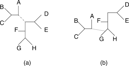
If we choose to add a topology a random n-taxa unrooted tree is generated from the prior. When removing a state we choose at random. When updating an existing topology we choose randomly and perform a local rearrangement by selecting a branch in the tree and cutting it. The two resulting subtrees are then joined together with a new branch (Fig. 1). The resulting model is accepted or rejected according to the Metropolis-Hastings ratio:

(13)

Since we do not propose parameters that change across dimension, the Jacobian is equal to 1.

Fig. 1.

When we choose to update an existing topology, we perform a local rearrangement. A branch in the tree is selected [the dashed branch in subplot (a)] and this branch is removed. The resulting subtree is rejoined to the main tree at a new location [via the dotted branch in subplot (b)]

For the sampling step in (8), we again sample a path through the data, this time through the states of the rate HMM, using the algorithm of Boys et al. (2000). In order to update the ρ parameters we can sample from a beta distribution. Let C_T = ∑^L−1_i=1 δ (T_i,T_i+1) and C_R =; ∑^L−1_i=1 δ (R_i,R_i+1). Then

(14)

(15)

4 DATA

The proposed method has been tested on several datasets, both simulated and real. The datasets described below and the implemented method are available from http://www.stats.ox.ac.uk/~webb

4.1 Simulated data

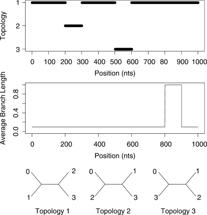
Initially we consider a 4-taxa dataset which was generated using the BARGE program of Husmeier (2005). This generated a 1000 bp alignment using the Kimura model of substitution. Two recombination events were simulated as well as a 100 bp region of increased branch lengths of the topologies as shown in Figure 2. Full details of the simulation are given in Husmeier (2005).

Fig. 2.

Simulated recombination in a 4-species alignment. A change in topology is simulated between sites 200 and 300 and between sites 500 and 600. The average branch length of the topologies is increased by a factor of 10 between sites 800 and 900.

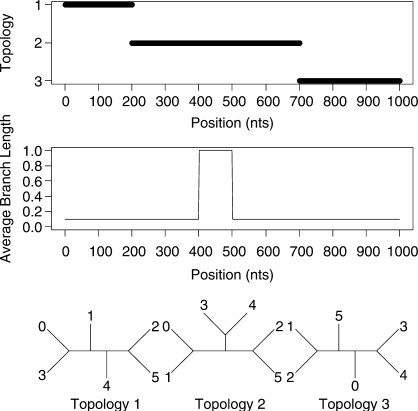
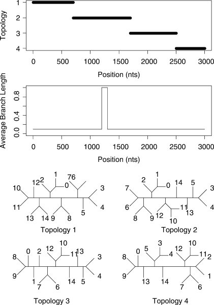
We will also consider two datasets with more than four taxa. A 6-taxa dataset of length 1000 bp and a 15-taxa dataset of length 3000 bp were both generated using the program SeqGen of Rambaut and Grassly (1997). Data were simulated under an HKY model of mutation with a stationary distribution of (0.1, 0.4, 0.4 and 0.1) for the four nucleotides and a transition transversion ratio of 2.0. Rate heterogeneity was incorporated into the simulation by assigning different branch lengths in different parts of the tree. The average branch length for most of the alignment was 0.1 but each dataset contains a 100 bp region where the average length is increased to 1.0. The topologies and rates used to simulate the data are shown in Figure 3 and Figure 4 for the 6-taxa and 15-taxa datasets, respectively. As mentioned by a reviewer, our inference of recombination will be affected by the rate of substitution. This is explored in the Supplementary Materials.

Fig. 3.

Simulated recombination in a 6-species alignment. A change in topology is simulated at sites 200 and 700. The average branch length undergoes a 10-fold increase between sites 400 and 500.

Fig. 4.

Simulated recombination in a 15-species alignment. A change in topology is simulated at sites 700, 1700 and 2500. The relative rate of evolution undergoes a 10-fold increase between sites 1200 and 1300.

The MCMC algorithm was run for 50 000 iterations with the first 25 000 discarded as burn-in. The ρ parameters were initialized to be ρ_T = ρ_R = 0.9, since we do not expect recombination events or changes in rate to be common in our alignment. The resulting samples are used to form our posterior distribution on the probability of each topology at each site of the alignment.

4.2 An HIV recombinant

As an application to a real dataset, we apply our method to the genome of an HIV-1 isolate, KAL153 (accession number AF193276). The isolate is aligned with consensus sequences of HIV-1 subtypes A, B and F since Liitsola et al. (1998) showed that KAL153 has genes originating from subtypes A and B. This dataset has previously been analyzed by (Minin et al., 2005) in their DualMCP method which will provide a useful comparison to our approach. The algorithm was again run for 50 000 iterations and 25 000 were taken as our sample from the posterior.

4.3 15 inbred mouse strains

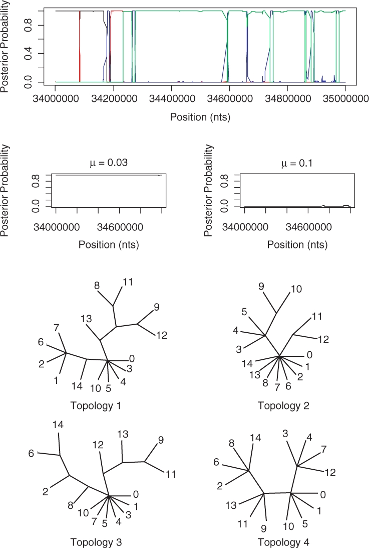
Finally, we consider SNPs spanning the genomes of 15 strains of mice. Recently Yang et al. (2007) and Frazer et al. (2007) studied these data and attempted to identify varying ancestral origin of the 11 classical strains using the wild-derived strains as reference sequences for each subspecies. We study a 1 Mb region of chromosome 4 which has been mapped for ancestral origin by Frazer et al. (2007). The results in Frazer et al. (2007) are presented as blocks representing which of the four wild types each of the classical strains is derived from (Fig. 2 of their paper). Due to the larger number of taxa the algorithm was run for 100 000 iterations with the final 25 000 being used to make our posterior sample.

5 RESULTS

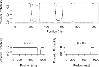
Figure 5 shows the predicted structure of the 4-taxa alignment using our Stochastic Topology HMM (STHMM). We have accurately recovered the locations of the changes in topology and evolutionary rate. The results are very similar to those of Husmeier (2005) for a similarly generated dataset. While this is not surprising, it does demonstrate the ability of the STHMM to infer recombination and rate heterogeneity correctly. The posterior probability shown in the figure is calculated as the average number of times each topology is present in the sampled path for each site of the alignment. The posterior probabilities are close to 1 for Topology 1 for most of the alignment and we see an obvious change in probability at the appropriate points giving us high confidence in the ability of the method to predict the changepoints.

Fig. 5.

Results from the 4-taxa data simulated using the BARGE program of Husmeier (2005). The solid line corresponds to topology 1, the dashed line to topology 2 and the dotted line to topology 3. We have successfully recovered the recombination events. The bottom plots show the posterior probability for the different states in the rate HMM. The values of the average branch length are restricted to {0.001, 0.003, 0.01, 0.03, 0.1, 0.3, 1.0, 3.0, 10.0, 100.0}. Only rates with a posterior P ≥ 0 are shown in the plot. The proposed method has picked up a change in rate between sites 800 and 900.

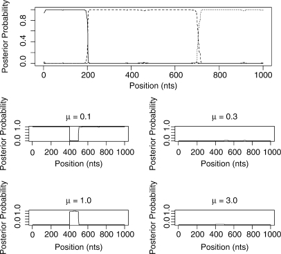
Our main goal is to be able to go beyond the case of 4-species alignments. Figure 6 shows the outcome of the STHMM when run on the simulated data for six taxa. Again we have successfully recovered the true trees under which the data were simulated as well as the changepoints for the factorial HMM. The STHMM was run on 100 replicates of the data to test for consistency. The average breakpoint location was taken across all samples in all runs and is shown in Table 1. In each of the 100 replicates, the true topologies used to generate the data were recovered by the STHMM. The method seems robust to other types of rate heterogeneity. Results are shown in the Supplementary Materials.

Fig. 6.

Results from the 6-taxa data simulated using the SeqGen program of Rambaut and Grassly (1997). The solid line corresponds to topology 1, the dashed line to topology 2 and the dotted line to topology 3. We have successfully recovered the recombination events. The bottom plots show the posterior probability for the different states in the rate HMM as described in Figure 5. We have inferred a change in rate between sites 400 and 500.

Table 1.

Average breakpoint locations from 100 replicates of the 6-taxa and 15-taxa simulated data

	Breakpoint 1	Breakpoint 2	Breakpoint 3
6 Taxa	198.97 (0.83)	702.59 (0.47)	−
15 Taxa	701.95 (0.61)	1696.45 (2.62)	2499.56 (0.56)

The averages for the 15-taxa data were taken over the datasets which contained that breakpoint (Table 2). The standard errors are shown in brackets.

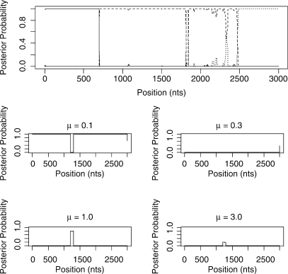
Figure 7 shows the inferred structure from the 15-taxa simulation. Again the STHMM has managed to recover the change in rate between sites 1200 and 1300. The changes in topology presented more of a problem here, due to the vastly increased state space (7, 905, 853, 580, 625 possible unrooted trees). We have not managed to detect all the breakpoints. Where one of the breakpoints is not located, the regions that are joined into one are represented by one ‘compromise’ topology. Table 1 shows the average breakpoint locations from 100 replicates and Table 2 shows the proportion of times we recover a breakpoint at approximately the correct location (within 50 bp) and the average Robinson-Foulds distance between the inferred and true trees. This should give us a measure of how close our trees are to the ones used to generate the data. The Robinson-Foulds distance was calculated using the Split-Dist program of Mailund (2003). Since the state space is so large it is likely that we have not been able to propose the true trees underlying the data. In fact, if the ST-HMM algorithm is initialized with the four correct topologies it maintains them throughout and the likelihood is higher than that reached in any replicate where the truth is not recovered. Ideally, we would be able to propose to add new trees to the topology HMM that can be reached in one recombination event from an existing tree in the model. This idea is discussed in the Discussion section.

Fig. 7.

Results from one run of the STHMM on the 15-taxa data simulated using the SeqGen program of Rambaut and Grassly (1997). We have inferred, correctly, a breakpoint at positions 700 and 2500, however we are not certain of the topology between sites 1700 and 2500. The trees inferred in this example are correct except for the region 3 tree which has a Robinson-Foulds distance of 3 from the true tree. The bottom plots show the posterior probability for the different states in the rate HMM as described in Figure 5. We have correctly inferred a change in rate between sites 1200 and 1300.

Table 2.

Proportion of times each breakpoint was located and the average Robinson-Foulds distance between the inferred and true trees for each region over 100 replicates of the 15-taxa simulated data

Breakpoint 1	Breakpoint 2	Breakpoint 3
0.88	0.51	0.81
Topology 1	Topology 2	Topology 3	Topology 4
0.3 (0.09)	0.75 (0.11)	1.15 (0.13)	0.8 (0.18)

The standard error for the Robinson-Foulds distance is shown in brackets.

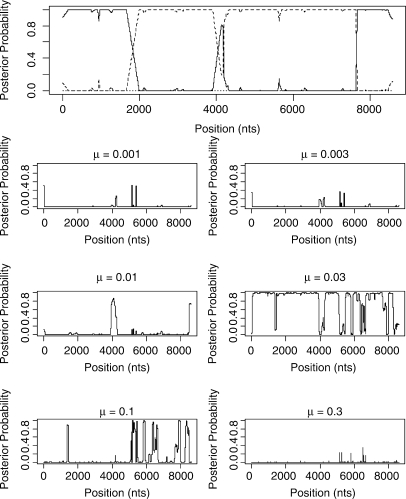
We now apply the STHMM to two real datasets, one alignment of four HIV strains which has been studied in Minin et al. (2005) and SNP data from 15 strains of inbred laboratory mice that have been investigated for variation in ancestral origin by Frazer et al. (2007). The results for the HIV-1 alignment are shown in Figure 8. Subtypes A and B correspond to the taxon labels 1 and 2, respectively, and the KAL153 isolate is taxon 3. As we can see, the inferred structure of the suspected recombinant is (A,B,A,B,A). This is very similar to the result from the DualMCP (Minin et al., 2005). However, we infer a change in topology at around site 4000 which is not inferred by the DualMCP.

Fig. 8.

Results from the KAL153 isolate. The solid line corresponds to topology 1, the dashed line to topology 2 and the dotted line to topology 3 as in Figure 2. The inferred recombinant structure is (A,B,A,B,A).

Figure 9, shows the results for the 15 inbred mouse strains. In Frazer et al. (2007), a HMM is created with five states, one for each of the four ancestral strains and a state representing unknown origin. Each SNP for each classical strain is then assigned to one of these states by using the Viterbi algorithm. The STHMM is very consistent with the positions of the recombination breakpoints. However, it seems unable to resolve several of the splits in the tree and hence explores a large number of similar trees and we end up assigning a small posterior probability to many of them. To illustrate the results, we have therefore collected together the probabilities for several trees and represented them with a single tree with multifurcations.

Fig. 9.

Results from the 15 inbred mouse strains. The trees output by the STHMM have been collected together into trees with multifurcations. The lines correspond to the following topologies: black—1, red—2, blue—3, green—4. The labels on the trees refer to the strains: 0—DBA/2J, 1—A/J, 2—BALB/cByJ, 3—C3H/HeJ, 4—AKR/J, 5—FVB/NJ, 6—129S1/SvImJ, 7—NOD/LtJ, 8—WSB/EiJ, 9—PWD/PhJ, 10—BTBR T+ tf/J, 11—CAST/EiJ, 12—MOLF/EiJ, 13—NZW/LacJ and 14—KK/HlJ. The trees were drawn using the TreeView program of (Page, 1996).

While our results are not directly comparable to those of Frazer et al. (2007) since they only classify the 11 classical strains according to which of the four ancestral strains they are closest to at each point, there are similarities which lead us to believe that our results are meaningful. For example, in Figure 2 of Frazer et al. (2007) the strains BALB/cByJ, 129S1/SvImJ and KK/HlJ seem to share a similar pattern of ancestry. As we can see from our topologies in Figure 9, taxa 2, 6 and 14 are grouped together consistently. Also, strain NZW/LacJ undergoes a change in ancestry from WSB/EiJ to PWD/PhJ in the method of Frazer et al. (2007). We see a change in our topologies where strain 13 is closer to strain 9 than strain 8 for topologies 3 and 4. The advantage of our method is that we are able to quantify our uncertainty at each position, since we consider the posterior probability of each topology rather than the single most likely outcome. We are also able to give greater detail of the ancestry of the mouse strains as we provide a topology relating all 15 strains instead of just considering which ancestral strain is the most similar to each of the 11 classical strains.

6 DISCUSSION

We have developed a STHMM for inferring recombination breakpoints and rate heterogeneity and estimating the relationships between species. We have also successfully applied it to several datasets, both simulated and real. We are able to investigate problems beyond four taxa by not considering all possible phylogenies but instead focusing our stochastic search on trees with high posterior probability. Our method allows us to take advantage of the structure of HMMs to sample over all possible breakpoints using the stochastic Forwards-Backwards algorithm, assuming sufficient MCMC iterations. Therefore, we reduce the dimensionality of the problem by only needing to explore trees as opposed to breakpoint locations and trees as in Suchard et al. (2003) and Minin et al.(2005). The advantage of our method is that we take account of the uncertainty by allowing the data to dictate how many topologies we require and the most probable locations for the breakpoints.

One problem we did encounter was the difficulty for the method to detect breakpoints between trees which are very similar. One way to deal with this may be to allow both local and global trees to be proposed when we choose to add a new tree to the topology HMM. Global trees could be suggested from the prior; whereas, local trees would be restricted to be one ‘subtree prune and regraft’ move away from an existing tree. This would require us to be able to calculate the probability of proposing a particular topology given the set of topologies already in the HMM. An algorithm for calculating the approximate ‘SPR distance’ between two trees is proposed in de Oliveira Martins et al. (2008). This might enable a more focused search of the tree space although one must be careful to ensure that the probabilities of moving between trees take account of all possible paths between states.

For this analysis, we have fixed the rate HMM to contain a specified number of states. However, it would be possible to use a similar approach as for the topology HMM where we can add and remove states using reversible-jump MCMC (Green, 1995; Lehrach and Husmeier, 2008). This would be easy to implement, given the current structure but would add computational time since we would expect the MCMC to take longer to converge.

REFERENCES

- Boys RJ, et al. Detecting homogeneous segments in DNA sequences by using hidden Markov models. Appl. Stat. 2000;49:269–285. [Google Scholar]
- de Oliveira Martins L, et al. Phylogenetic detection of recombination with a Bayesian prior on the distance between trees. PLoS ONE. 2008;3 doi: 10.1371/journal.pone.0002651. [DOI] [PMC free article] [PubMed] [Google Scholar]
- Felsenstein J. Evolutionary trees from DNA sequences: a maximum likelihood approach. J. Mol. Evol. 1981;17:368–374. doi: 10.1007/BF01734359. [DOI] [PubMed] [Google Scholar]
- Felsenstein J. PHYLIP (Phylogeny Inference Package) version 3.6. Seattle: Department of Genome Sciences, University of Washington; 2005a. [Google Scholar]
- Felsenstein J. Inferring Phylogenies. Sinauer Associates, Inc; 2005b. [Google Scholar]
- Frazer KA, et al. A sequence-based variation map of 8.27 million SNPs in inbred mouse strains. Nature. 2007;448:1050–1053. doi: 10.1038/nature06067. [DOI] [PubMed] [Google Scholar]
- George EI, McCulloch RE. Stochastic search variable selection. In. In: Gilks WR, et al., editors. Markov Chain Monte Carlo in Practice. Chapman & Hall; 1995. pp. 203–214. [Google Scholar]
- Grassly NC, Holmes EC. A likelihood method for the detection of selection and recombination using nucleotide sequences. Mol. Biol. Evol. 1997;14:239–247. doi: 10.1093/oxfordjournals.molbev.a025760. [DOI] [PubMed] [Google Scholar]
- Green PJ. Reversible jump markov chain monte carlo computation and Bayesian model determination. Biometrika. 1995;82:711–732. [Google Scholar]
- Hasegawa M, et al. Dating the human-ape splitting by a molecular clock of mitochondrial DNA. J. Mol. Evol. 1985;22:160–174. doi: 10.1007/BF02101694. [DOI] [PubMed] [Google Scholar]
- Hobolth A, et al. Genomic relationships and speciation times of human, chimpanzee, and gorilla inferred from a coalescent hidden Markov model. PLoS Genet. 2007;3:294–304. doi: 10.1371/journal.pgen.0030007. [DOI] [PMC free article] [PubMed] [Google Scholar]
- Husmeier D. Discriminating between rate heterogeneity and interspecific recombination in DNA sequence alignments with phylogenetic hidden Markov models. Bioinformatics. 2005;21:166–172. doi: 10.1093/bioinformatics/bti1127. [DOI] [PubMed] [Google Scholar]
- Husmeier D, McGuire G. Detecting recombination with MCMC. Bioinformatics. 2002;18:S345–S353. doi: 10.1093/bioinformatics/18.suppl_1.s345. [DOI] [PubMed] [Google Scholar]
- Husmeier D, McGuire G. Detecting recombination in 4-taxa DNA sequence alignments with Bayesian hidden Markov models and Markov chain Monte Carlo. Mol. Biol. Evol. 2003;20:315–337. doi: 10.1093/molbev/msg039. [DOI] [PubMed] [Google Scholar]
- Husmeier D, Mantzaris A. Addressing the shortcomings of three recent Bayesian methods for detecting interspecific recombination in DNA sequence alignments. Stat. Appl. Genet. Mol. Biol. 2008 doi: 10.2202/1544-6115.1399. [DOI] [PubMed] [Google Scholar]
- Lehrach W, Husmeier D. Segmenting bacterial and viral DNA sequence alignments with a transdimensional phylogenetic factorial hidden Markov model. Appl. Stat. 2008 [Google Scholar]
- Liitsola, et al. An AB recombinant and its parental HIV type 1 strains in the area of the former Soviet Union: low requirements for sequence identity in recombination. AIDS Res. Hum. Retroviruses. 1998;16:1047–1053. doi: 10.1089/08892220050075309. [DOI] [PubMed] [Google Scholar]
- Mailund T. Split-Dist – calculating split-distances for sets of trees. 2003 Available at http://www.daimi.au.dk/~mailund/split-dist.html.
- McGuire G, et al. A graphical method for detecting recombination in phylogenetic data sets. Mol. Biol. Evol. 1997;14:1125–1131. doi: 10.1093/oxfordjournals.molbev.a025722. [DOI] [PubMed] [Google Scholar]
- McGuire G, Wright F. TOPAL 2.0: improved detection of mosaic sequences within multiple alignments. Bioinformatics. 2000;16:130–134. doi: 10.1093/bioinformatics/16.2.130. [DOI] [PubMed] [Google Scholar]
- Minin VN, et al. Dual multiple change-point model leads to more accurate recombination detection. Bioinformatics. 2005;21:3034–3042. doi: 10.1093/bioinformatics/bti459. [DOI] [PubMed] [Google Scholar]
- Page RDM. TREEVIEW: an application to display phylogenetic trees on personal computers. Comput. Appl. Biosci. 1996;12:357–358. doi: 10.1093/bioinformatics/12.4.357. [DOI] [PubMed] [Google Scholar]
- Pattengale ND, et al. Efficiently computing the robinson-foulds metric. J. Comput. Biol. 2007;14:724–735. doi: 10.1089/cmb.2007.R012. [DOI] [PubMed] [Google Scholar]
- Rabiner LR. A tutorial on hidden Markov models and selected applications in speech recognition. Proc. IEEE. 1989;77:257–286. [Google Scholar]
- Rambaut A, Grassly NC. Seq-Gen: an application for the Monte Carlo simulation of DNA sequence evolution along phylogenetic trees. Comput. Appl. Biosci. 1997;13:235–238. doi: 10.1093/bioinformatics/13.3.235. [DOI] [PubMed] [Google Scholar]
- Schierup MH, Hein J. Consequences of recombination on traditional phylogenetic analysis. Genetics. 2000;156:879–891. doi: 10.1093/genetics/156.2.879. [DOI] [PMC free article] [PubMed] [Google Scholar]
- Suchard MA, et al. Inferring spatial phylogenetic variation along nucleotide sequences: a multiple changepoint model. J. Am. Stat. Assoc. 2003;98:427–437. [Google Scholar]
- Yang H, et al. On the subspecific origin of the laboratory mouse. Nat. Genet. 2007;39:1100–1107. doi: 10.1038/ng2087. [DOI] [PubMed] [Google Scholar]
Associated Data
This section collects any data citations, data availability statements, or supplementary materials included in this article.