FastMap: Fast eQTL mapping in homozygous populations

Abstract

Motivation: Gene expression Quantitative Trait Locus (eQTL) mapping measures the association between transcript expression and genotype in order to find genomic locations likely to regulate transcript expression. The availability of both gene expression and high-density genotype data has improved our ability to perform eQTL mapping in inbred mouse and other homozygous populations. However, existing eQTL mapping software does not scale well when the number of transcripts and markers are on the order of 10⁵ and 10⁵–10⁶, respectively.

Results: We propose a new method, FastMap, for fast and efficient eQTL mapping in homozygous inbred populations with binary allele calls. FastMap exploits the discrete nature and structure of the measured single nucleotide polymorphisms (SNPs). In particular, SNPs are organized into a Hamming distance-based tree that minimizes the number of arithmetic operations required to calculate the association of a SNP by making use of the association of its parent SNP in the tree. FastMap's tree can be used to perform both single marker mapping and haplotype association mapping over an m-SNP window. These performance enhancements also permit permutation-based significance testing.

Availability: The FastMap program and source code are available at the website: http://cebc.unc.edu/fastmap86.html

Contact: iir@unc.edu; nobel@email.unc.edu

Supplementary information: Supplementary data are available at Bioinformatics online.

1 INTRODUCTION

Quantitative Trait Locus (QTL) mapping is a set of techniques that locates genomic loci associated with phenotypic variation in a genetically segregating population. QTL mapping has been highly successful in determining causative loci underlying several disease phenotypes (Cervino et al., 2005; Hillebrandt et al., 2005; Wang et al., 2004) and can broadly be subdivided into two classes: linkage mapping and association mapping. For standard linkage mapping in experimental crosses, likelihood or regression approaches are used to map QTL, with flanking markers used to infer genotypes in the intervals between widely spaced markers (i.e. >1 cM) (Haley and Knott, 1992; Lander and Botstein, 1989). As marker density increases, linkage statistics may be computed at individual marker loci, with minimal loss in precision or power (Kong and Wright, 1994). In contrast, simple association mapping does not attempt to explicitly consider the linkage disequilibrium structure between marker loci, and thus typically considers association statistics computed only at the marker loci. In either case, the statistics computed at the markers in experimental cross-linkage designs, and in association studies, are often identical, e.g. t-statistics to detect differences in phenotype means as a function of genotype. Here, we consider the case of markers collected at sufficient density so that association statistics may be calculated only at the observed markers.

Recent advances in gene expression and single nucleotide polymorphism (SNP) microarray technology have lowered the cost of collecting gene expression and high-density genotype data on the same population. These technologies have been used to produce high-density SNP datasets with thousands of transcripts and millions of allele calls in both mice (Frazer et al., 2007b; Szatkiewicz et al., 2008) and humans (Frazer et al., 2007a). eQTL mapping has been successfully carried out in several inbred mouse populations (Bystrykh et al., 2005; Chesler et al., 2005; Gatti et al., 2007; McClurg et al., 2007; Pletcher et al., 2004; Schadt et al., 2003). These studies have provided a revealing genome-wide view of the genetic basis of transcriptional regulation in multiple tissues, and form a necessary foundation for systems genetics (Kadarmideen et al., 2006; Mehrabian et al., 2005).

The calculation of associations between tens of thousands of transcripts and thousands to millions of SNPs creates a computational challenge that can stretch or overwhelm existing tools. These challenges are further compounded by multiple comparison issues arising from the large number of available SNPs and transcripts. Various methods have been used to address these issues. A resampling approach (Carlborg et al., 2005; Churchill and Doerge, 1994; Peirce et al., 2006) is one common way of addressing multiple comparisons among markers, and it is used by several available QTL mapping tools (Broman et al., 2003; Manly et al., 2001; Wang et al., 2003). Multiple comparisons among transcripts has been previously addressed by thresholding transcripts using q-values (Storey and Tibshirani, 2003) obtained from transcript-specific testing of association with SNPs using Likelihood Ratio Statistic (LRS) (Chesler et al., 2005) or the mixture over markers method (Kendziorski et al., 2006).

While parallel computation has been suggested as a potential solution to the computational challenges associated with eQTL analysis (Carlborg et al., 2005), many researchers have neither the expertise nor the resources required to administer and maintain a computing cluster. To address the growing need for eQTL mapping in high-density SNP datasets, and the poor scalability of the existing computational tools, we developed the FastMap algorithm and implemented it as a Java-based, desktop software package that performs eQTL analysis using association mapping. We achieve computational efficiency through the use of a data structure called a Subset Summation Tree, which is described in Section 2 below. FastMap performs either single marker mapping (SMM) or haplotype association mapping (HAM) by sliding an m-SNP window across the genome (Pletcher et al., 2004). FastMap is currently intended for the use with inbred mouse strains. Significance thresholds and p-values are calculated for each transcript using multiple permutations of transcript expression values. In order to address multiple comparisons across transcripts, FastMap assigns a q-value (Storey and Tibshirani, 2003) assessing FDR, to each transcript. We apply our software tool to two publicly available datasets consisting of gene expression measurements in panels of inbred mice and compare our results to other software tools.

2 METHODS

This section first describes the calculations of test statistics (correlations) for SMM in a 1-SNP sliding window. First we introduce the concept of a subset sum M_g(s) and a Subset Summation Tree. Subset sums are quantities that can be efficiently calculated using the Subset Summation Tree, and are used in the calculation of correlations. We then show how the subset sums and Subset Summation Tree can be adapted to the fast calculation of ANOVA test statistics for m-SNP sliding windows (m>1).

In association mapping for homozygous inbred strains, the input data consists of two matrices: the first contains real-valued transcript expression measurements and the second contains SNP allele calls, coded as 0 for the major allele and 1 for minor allele. Each matrix has the same number of samples (strains) n. Let S be the number of SNPs and let G be the number of transcripts.

Homozygous SNPs: 1-SNP window: we use the Pearson correlation as an association statistic in the case of a 1-SNP window. For a given transcript g and SNP s the correlation between g and s is

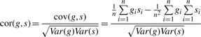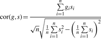
To simplify the formula, we assume without loss of generality that each transcript expression vector g is centered and standardized such that

(1)

In this case, the correlation expression reduces to

The denominator can be calculated once for each SNP, because it depends only upon the Hamming weight of s. In contrast, the numerator must be calculated for every SNP–transcript pair (S × G computations). Our goal is to speed up calculation of the numerator. Denote the numerator by M_g(s):

As the SNPs are binary, M_g(s) is simply the sum of transcript expression values over a subset of samples defined by the minor allele of the SNP.

To illustrate how the calculation of the M_g(s) can be simplified, consider two SNPs s and s′ that differ only at the i-th position (thus s and s′ have Hamming distance of 1):

In this case, the quantity M_g(s′) can be calculated quickly (in one arithmetic operation) from M_g(s) as follows:

(2)

For any given transcript, the association statistic is the same for SNPs with the same strain distribution pattern (SDP). Hence, we calculate the association statistic once for each unique SDP. The McClurg mouse data used in this article contains 156 525 SNPs, but has only 64 157 unique SDPs.

Additional improvements are based on Formula (2). To take full advantage of this relationship between correlations, we construct a tree, which we call a Subset Summation Tree. The vertices of the tree correspond to unique subsets of samples. Each SDP defines a subset of samples associated with its minor allele. The tree contains all SDPs appearing in the SNP matrix. By construction, the edges of tree connect SDPs which differ in one position (i.e. Hamming distance 1). The process of tree construction is described later in this section. It ensures that the tree is at least as efficient (in terms of weight based on the Hamming distance) as the minimum spanning tree connecting all SDPs from the SNP matrix. An illustration of a subset summation tree is given in Figure 1.

Fig. 1.

The Subset Summation Tree is used to calculate the covariance sums in Pearson's correlation statistic. The table shows one gene expression vector and six corresponding SNP vectors for seven strains. At each node, the covariance of the gene expression with each SNP is calculated with one addition operation.

Traversing the tree we can calculate the covariance M_g(s) for all SDPs in the tree with one arithmetic operation per SDP. One additional arithmetic operation is required to calculate the correlation from M_g(s).

Homozygous SNPs: m-SNP sliding window: The use of a consecutive 3-SNP sliding window has been shown to improve the associations that can be detected in mouse studies (Pletcher et al., 2004). FastMap is capable of employing any m-SNP window specified by the user. Within each m-SNP window, the strains form haplotypes that partition strains into ANOVA groups. A one way ANOVA test statistic is then used to assess the relationship between a gene g and an m-SNP window.

Consider a 3-SNP window that contains k unique haplotype (ANOVA) groups across the n stains. Let A_i denote the set of samples in the i-th ANOVA group, and let the transcript expression values in the i-th ANOVA group be g_ij,j=1,…,n_i. The associated ANOVA test statistic is calculated as

where the between group sum of squares SSB, and within group sum of squares SSW are calculated as follows:

The sums of squares are related by SST=SSB+SSW.

For a given transcript, the total sum of squares (SST) remains constant across all SNPs. As in the 1-SNP window case, the gene expression values are standardized to satisfy the conditions in Equation (1). For standardized expression measurements, the SST and SSB calculations simplify as follows:

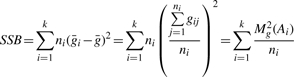where M_g(A_i) is sum of the transcript expression values for the i-th ANOVA group. As before, M_g(A_i) can be calculated efficiently using the Subset Summation Tree. The difference is that the tree for these calculations connects subsets of samples defining the m-SNP ANOVA groups, as opposed to SDPs defined by single SNPs. Once the SSB is calculated, the F-statistic is calculated as:

Tree construction: The Subset Summation Tree is used for fast calculation of M_g(A_i)—sums of transcript expression values over subsets of samples {A_i}. Tree construction is initiated by obtaining the family of sample subsets of interest {A_i} from the set of SNPs. The tree is grown starting from single root element (empty subset) by sequential addition of the nearest element from {A_i} to the tree.

All the subsets {A_i} are put in a hash table (HT) that stores the subsets that are not yet members of the tree. The tree is grown by connecting subsets that are at the minimum distance from the tree. Node selection and connection to the tree can be optimized by taking advantage of two facts. First, the Hamming distances are positive integers. Thus, once we find a subset in the HT within distance 1 of a particular tree vertex, we connect them, adding the subset to the tree and removing it from the HT. To find such an SDP in the HT we use the second fact: for any subset, there are only n possible subsets that are within hamming distance 1 from it. Thus, instead of calculating distances from a certain tree vertex to all subsets in the HT we can check if the HT contains any of the n possible neighbor subsets. This approach reduces the complexity of the search for close (within distance 1) neighbors of a given tree vertex from O(nS) to O(n).

The procedure above is applicable as long as there are SDPs in the HT within distance 1 from the tree. Once there are no SDPs in the HT within distance 1 from tree vertices, the search continues for SDPs within distance 2. The same optimizations are applicable here—once an SDP within distance 2 is found, it should be connected to the tree and there are n(n−1)/2 possible SDPs within distance 2 from a given tree vertex. The same technique is applied even for the search for subsets within distance 3. When the remaining vertices are at Hamming distance 4 or greater, an exhaustive search is performed to find a node in HT that is a minimum distance from the tree. This process is repeated until all SNPs have been inserted into the tree.

Permutation-based significance thresholds: for a single transcript, the association statistic is calculated between the observed values of that transcript and all SNPs. The transcript data are then permuted while the SNP data are held fixed. Association statistics are calculated between the permuted transcript values and all SNPs and the maximum association statistic is stored. The distribution of the maximum association statistics obtained from 1000 permutations of the transcript's values is used to define significance thresholds for individual (transcript, SNP) pairs, and to assign a percentile-based p-value to the observed maximum association of the transcript across SNPs.

Significance across multiple transcripts: the procedure above assigns a p-value to each transcript that accounts for multiple comparisons across SNPs through the use of the maximum association statistic. In order to correct for multiple comparisons across transcripts, we calculate q-values (Storey and Tibshirani, 2003) for each transcript, using the p-values obtained from the permutation-based maximum association test.

2.1 Data

2.1.1 BXD gene expression data

The BXD Liver dataset is available from genome.unc.edu, and is described in Gatti et al. (2007). Briefly, it consists of microarray-derived expression measurements for 20 868 transcripts in 39 BXD recombinant inbred strains and the C57BL/6J and DBA/2J parentals. The data were normalized using the UNC Microarray database and QTL analysis was performed on all transcripts.

2.1.2 BXD marker data

The BXD marker data consist of 3795 informative markers taken from a larger set of 13 377 markers. Briefly, consecutive markers with the same SDP were removed and only the flanking markers of such regions were included. The data were downloaded from http://www.genenetwork.org/genotypes/BXD.geno; further information is available at http://www.genenetwork.org/dbdoc/BXDGeno.html.

2.1.3 Hypothalamus gene expression data

The mouse hypothalamus dataset GSE5961 was downloaded from the NCBI Gene Expression Omnibus website. These data are described in McClurg et al. (2007). The 58 CEL files were normalized using the gcrma package from Bioconductor (version 1.9.9) in R (version 2.4.1). The data were subset to include only the 31 male samples, and removing the NZB data because the entire array appeared as an outlier in hierarchical clustering of the arrays. There were 36 182 probes on the array; of these a subset of 3672 transcripts having an expression value >200 and at least a 3-fold difference in expression in one strain were selected. Transcripts containing a single outlier strain with expression values >4 SDs from the mean were removed from the dataset. There were 402 such transcripts, leaving 3270 transcripts for analysis in FastMap.

2.1.4 Hypothalamus SNP data

The SNP data were obtained from McClurg et al. (2007) and originally contained 71 inbred strains. Missing genotype data were imputed using the algorithm of Roberts et al. (2007a). There were 156 525 SNPs, of which 99 were monomorphic across the 32 strains. These SNPs were removed from the analysis, leaving 156 426 SNPs. There were 64 790 unique SDPs in this final dataset.

2.2 Settings

In Section 3.2, we compare FastMap performance with two other publicly available tools: SNPster (McClurg et al., 2006) and R/qtl (Broman et al., 2003). The setting used to run them are detailed below.

2.2.1 Snpster settings

SNPster runs were performed using the tool available at snpster.gnf.org. The following settings were selected and are listed in the order in which they appear on the website. (i) Log transform data: No. (ii) Test statistic: F-test. (iii) Method of calculating significance: parametric. (iv) Compute gFWER: No. The default settings were used for the remaining options on the web site.

2.2.2 R/qtl settings

R/qtl version 1.08-56 for R 2.7 was used to perform eQTL analysis on the BXD Liver dataset. R/qtl was configured to perform Haley–Knott regression only at the observed markers. eQTL significance was determined by performing 1000 permutations for each transcript and selecting only those eQTLs above the 95% LOD threshold.

2.2.3 Computer for performance testing

A Pentium 4 with a clock speed of 3.4 GHz and 4 GB of RAM running Microsoft Windows XP Professional(r), SP2 was used for all timing runs. No other applications were open during the runs.

3 RESULTS AND DISCUSSION

3.1 FastMap application

FastMap is written in the Java programming language and is driven by a simple graphical user interface (GUI, Fig. 2a). The required input files are (i) a transcript expression file with mean expression values for each mouse strain and (ii) a SNP file containing allele calls for all strains, with the major and minor alleles coded as 0 and 1, respectively. Once the SNP file has been loaded, FastMap constructs a Subset Summation Tree (see Section 2) for the SNP data, a computational task that is performed only once for a given set of strains. FastMap allows the user to perform either SMM by calculating the Pearson correlation of each transcript expression measurement with each SNP, or HAM by sliding an m-SNP window across the genome and calculating the ANOVA F-statistic for the phenotype versus the distinct haplotypes observed in the window (Pletcher et al., 2004). The association statistic at each SNP is displayed in a zoomable panel that links to the University of California at Santa Cruz Genome Browser (Kent et al., 2002; Pontius et al., 2007) (Fig. 2b and c). Association plots may be exported as text files or as images.

Fig. 2.

FastMap application GUI. (a) FastMap with a list of probes on the left and the QTL plot on the right. (b) A zoomed in view of the significant QTL on Chr 1. (c) The same region in the UCSC Genome browser, to which FastMap can connect.

QTL mapping with sparsely distributed markers has traditionally used maximum likelihood methods and has employed the LRS or the related Log of the Odds ratio (LOD) as a measure of the association between genotype and phenotype [LRS=2ln(10)×LOD]. When marker density is high, regression techniques applied only at the observed markers will produce results which are numerically equivalent to the LRS or LOD (Kong and Wright, 1994). In fact, the LRS, Student t-statistic, Pearson correlation and the standard F-statistic, can be shown to be equivalent when they are applied at the marker locations (Supplementary Material). While previous literature has shown that regression methods produce estimates with a higher mean square error and have less power (Kao, 2000), these results apply primarily to the case of interval mapping when the spacing between markers is wide (>1cM). For these reasons, FastMap employs the Pearson correlation for SMM and the F-statistic for HAM when employing high-density SNP datasets.

The significance of eQTLs for a single transcript may be determined using a permutation-based approach (Churchill and Doerge, 1994). The expression values of each transcript are permuted, the association statistics of each transcript with all SNPs are calculated and the maximum transcript-specific association statistic is retained. This process is repeated 1000 times, and a significance threshold is taken as the 1−α percentile of the empirical distribution of the maxima. Both the number of permutations and the significance thresholds may be specified by the user. Since the various association statistics are equivalent when applied at the markers, the significant marker locations will be the same for any choice of these statistics. Once a QTL peak that exceeds a user selected threshold has been identified, the width of the QTL must be defined in order to identify potential candidate genes for further study. Given a local maximum d, a confidence region can be defined as all markers q in an interval around d such that 2ln(LR(q))≥max_d 2ln(LR(d))−x and this interval is referred to as an (x/2ln10)-LOD support interval (Dupuis and Siegmund, 1999). The choice of x=4.6 yields a 1-LOD confidence interval, which has been widely used in linkage analysis. A more conservative choice of x=6.9 (a 1.5-LOD interval) is more appropriate to situations with dense markers, yielding approximate 95% coverage under dense marker scenarios. Intervals for non-LR association statistics can be calculated from the relationships between statistics provided in the Supplementary Material. In practice, eQTL peak regions are limited by the effective resolution determined by breeding and recombination history.

FastMap assigns a p-value to each transcript that indicates the significance of the maximum association of that transcript across all the available markers. In situations where it is necessary or of interest to simultaneously consider multiple transcripts, additional steps must be taken to account for the resulting multiple comparison problem. We address this by calculating the q-value (Storey and Tibshirani, 2003) of every transcript. The q-value of a transcript is related to the false discovery rate. In particular, the q-value of a transcript is an estimate of the fraction of false discoveries among transcripts that are equally or more significant than it is. For example, if we create a list of transcripts consisting of a transcript with q-value equal to 10%, and all those transcripts having smaller permutation-based values, then we expect 10% or less of the transcripts on the list to have a significant association with at least on SNP or haplotype.

Permutation-based significance testing is frequently used in eQTL analysis (Doerge and Churchill, 1996; Peirce et al., 2006), and typically forms the bulk of the computational burden in eQTL mapping. It is natural to ask whether a parametric approach, based on Gaussian p-values, would be just as effective and save a significant amount of time. We note that permutation-based testing offers several advantages over parametric approaches. Permutation testing deals cleanly with the problem of multiple comparisons, and induces a null distribution under which there is no association between transcript expression and genotype, regardless of the underlying distributions from which the data are drawn, and the correlations between SNPs. In addition, the normality assumptions underlying parametric tests are often violated in practice.

3.2 Performance and speed

In order to gauge the performance improvement provided by FastMap over existing software, we compared computation times using two microarray datasets. The first consists of 20 868 transcripts and 3795 markers in 41 strains of mice [BXD dataset; (Gatti et al., 2007)]. This dataset was selected because, unlike the following larger dataset, it can be loaded into the widely used R/qtl package without exhausting computer memory. The second is a hypothalamus dataset (McClurg et al., 2006) that consists of 3672 transcripts, 156 525 markers in 32 strains of laboratory inbred mice. This dataset was selected for its dense genotype information, which is on the scale of the expected high-density SNP data for which we designed FastMap.

The amount of time required to perform eQTL mapping in these datasets is summarized in Table 1. In the BXD dataset, FastMap performs SMM for the entire set of 20 868 transcripts in about half an hour, which is the same time required for R/qtl to analyze 100 transcripts. The hypothalamus data were previously analyzed with an association mapping tool called SNPster (McClurg et al., 2006), which is available as a web application hosted by the Genomic Institute of the Novartis Research Foundation (GNF). A single transcript typically requires <5 min to analyze, depending on the load on SNPster's web server. However, obtaining results for thousands of transcripts from submissions to an external website is impractical in most cases. Another version of SNPster runs at GNF in parallel on a 200 node cluster, which is not publicly available, in batches of 10 transcripts per node. It requires 18 min to process these 10 transcripts using 1 000 000 bootstrap resamplings for each transcript, and a −log(P-value) threshold of 2.5, which implies ∼1.8 CPU-minutes per transcript (T.Wiltshire, personal communication). If these 3672 transcripts were analyzed serially rather than in parallel, this would require 110.2 h. In contrast, FastMap runs on a standard desktop computer and can perform eQTL mapping for these same 3672 transcripts with 156 K SNPs in 32 strains in 12.3 h. Large computing clusters, and the expertise required to administer them, are not available to all laboratories. FastMap offers the convenience of running on a single, local computer in a reasonable amount of time (overnight, or over a weekend for more than 10 000 transcripts).

Table 1.

FastMap eQTL mapping times

Software	DataSet	Method	Transcripts	Markers	Time (min)
R/qtl	BXD	LRS	100	3795	33.73
FastMap		SMM	20 868		29.95
SNPster	McClurg	HAM	3672	156 525	6609.6
FastMap					737.5

We evaluated the scalability of FastMap with increasing numbers of transcripts and SNPs using the hypothalamus dataset. Since we are aware of no stand-alone software that can perform eQTL mapping with hundreds of thousands of SNPs, we compared FastMap's performance in these plots to a brute force approach in which all calculations are performed without any optimizations. In the case of both SMM and HAM, computation time for FastMap scales linearly with increasing numbers of transcripts (Fig. 3a). FastMap also scales linearly with increasing number of SNPs (Fig. 3b).

Fig. 3.

FastMap scales linearly with increasing numbers of genes and SNPs. (a and b) The time required to compute the association of increasing numbers of transcripts with 156K SNPs. (c and d) The time required to compute the association of one transcript with increasing numbers of SNPs. In all four cases, 1000 permutations per transcript were performed.

In order to examine the scalability of our algorithm with increasing numbers of strains, we determined tree construction times for various sets of inbred strains genotyped at approximately 156 525 SNPs (Table 2). The amount of time required to construct the tree is a function of both the number of strains as well as their ancestral relationships. Strains that are closely related (i.e. all derived from Mus musculus domesticus (M.m.domesticus)) will produce nodes in the tree that are close to each other. As more distantly related strains are added (i.e. M.m.domesticus-derived strains combined with Mus musculus musculus (M.m.musculus)-derived strains), the distance between SDPs becomes larger and tree construction times increase. Most existing eQTL studies in panels of inbred strains have used less than 40 strains (Bystrykh et al., 2005; Chesler et al., 2005; McClurg et al., 2007). Tree construction required 5.3 min for the 32 strains of the hypothalamus dataset. In contrast, for a panel of 71 inbred strains derived from both M.m.domesticus and non-M.m.domesticus strains, tree construction requires ∼10 h using a 1-SNP window and ∼24 h using a 3-SNP window. Tree construction is carried out only once, and the resulting calculations still require less time than a brute force approach. Faster algorithms for tree construction that improve scalability with increasing numbers of strains are currently under investigation.

Table 2.

FastMap tree construction and association mapping times with increasing numbers of strains (in seconds)

	1-SNP window		3-SNP window
No. of Strains	Tree Constr.	SMM	Tree Constr.	HAP
16	1	0.05	8	2.8
32	168	2.5	320	12.9
54	3791	2.8	27 138	16.5
71	13 672	4.6	81 186	25.5

3.3 Population stratification

As noted by McClurg et al. (2007), considerable population stratification is present when panels of laboratory inbred strains are used. Common laboratory inbred strains are a mixture of M.m.domesticus, M.m.musculus, M.m.castaneus, M.m.molossinus and M. spretus, which arose during the creation of the laboratory inbred strains (Beck et al., 2000; Yang et al., 2007). Figure 4 shows a SNP similarity matrix for the 32 inbred strains in the hypothalamus dataset, where each cell represents the proportion of SNPs that have the same allele between two strains (normalized Hamming distance) across all 156K SNPs. The non-M.m.domesticus-derived strains cluster tightly in the lower left hand corner, indicating that they are more genotypicly similar to each other than to the M.m.domesticus-derived strains. Numerous transcripts and SNPs exhibit systematic differences across these two strata. Consequently, each such transcript will show a significant association with every such marker. In eQTL mapping, this produces numerous markers that show significant associations with the expression of a single transcript, leading to horizontal banding in the transcriptome map (Fig. 5a and b). When such differences exist, most permutations of the transcript will yield a lower association statistic than the observed one, this leads to inappropriately low significance thresholds (Fig. 5c). In order to remove this strata effect, we median center the values of each transcript within M.m.domesticus and non-M.m.domesticus strata. As shown in Figure 5d, the resulting transcriptome map becomes interpretable with cis-eQTLs along the diagonal. The few horizontal bands that remain are due to a subset of the M.m.musculus-derived strains with transcript expression levels that differ from the other strains; this prevents the median subtraction method from removing the strata effect completely. We recommend removing those few transcripts that demonstrate this effect.

Fig. 4.

SNP similarity matrix demonstrates population stratification among laboratory inbred strains. In one row, each cell represents the proportion of SNPs (in the 156K dataset) with the same allele in the other strains. The similarity matrix has been hierarchically clustered (distance=SNP similarity, linkage=average).

Fig. 5.

Strata median correction dramatically improves transcriptome map. (a) The transcriptome map for 3270 transcripts without correcting for the population structure for all eQTL above a transcript-specific 5% significance threshold. The horizontal bands dominate the plot and are due to gene expression profiles like the one in (b), which is marked by the red arrow in (a). The grey colored strains are the M.m.domesticus-derived strains and the red ones are the non-M.m.domestic-derived strains. By subtracting out the strata median from each strata, the transcriptome map (d) is greatly improved. Gene expression values are no longer split by genotypic strata (e) and the permutation-derived thresholds are appropriate (f).

FastMap allows the user to select strata by genotype a priori, and subtracts strata means or medians from the transcript values in each stratum (Pritchard et al., 2000). While there are more sophisticated methods for addressing population stratification (Kang et al., 2008), FastMap is not primarily designed to address this problem. While laboratory inbred strains have been useful in mapping Mendelian traits, eQTL mapping with FastMap will have greater utility in well-segregated populations like the Collaborative Cross (Churchill et al., 2004; Roberts et al., 2007b), due to increased genetic diversity, as well as the finer recombination block structure. In such well-mixed populations, mean/median subtraction within strata or the non-uniform resampling technique used by SNPster should not be required.

3.4 Comparison of FastMap to other QTL software

We compared the eQTL results produced by FastMap to those produced by R/qtl. R/qtl was configured to use Haley–Knott regression (Haley and Knott, 1992) and 1000 permutations to determine significance thresholds. While R/qtl is designed to perform linkage mapping, we note that when linkage mapping is performed exclusively at the markers, the calculations are identical to those performed in eQTL (Supplementary Material). eQTLs may be broadly separated into two categories; eQTLs located within 1 Mb of the transcript location (cis-eQTLs) and eQTLs located further than 1 Mb from the transcript location (trans-eQTLs). Both FastMap and R/qtl found similar numbers of total eQTLs, cis-eQTLs and trans-eQTLs (Fig. 6a). Figure 6b shows that the eQTL locations found by each software package are essentially identical; 98% of the eQTLs found by each method are within 5 Mb of each other, a margin of resolution consistent with the resolution of the BXD marker set. Since permutation-based testing involves randomization, it should not be expected that 100% of the eQTLs would match between the two methods. Furthermore, the eQTL histograms produced by each method (Fig. 6c and d) are similar, with differences being due to histogram binning effects (see insets).

Fig. 6.

FastMap eQTL mapping results almost equivalent to those obtained with R/qtl. (a) The BXD dataset and the number of matching eQTLs between FastMap and R/qtl at varying distances. (b) The high degree of concordance between FastMap and R/qtl. (c and d) eQTL histograms produced by FastMap and R/qtl. They are substantially equivalent with differences on Chr 1 and 12 being due to histogram binning effects (insets). Data are shown at 5% significance threshold.

eQTL mapping in the hypothalamus dataset was performed to evaluate computational performance, rather than to compare the results with SNPster. However, it is natural to ask how the results of the two methods compare when we employ median centering in FastMap to correct for population stratification. We correct for population stratification by median centering transcript values within M.m.domesticus-and non-M.m.domesticus-derived strains.

Since SNPster does not provide a fixed threshold for significance, we selected 2413 transcripts which had SNPster p-values <10⁻⁴. Of these, 105 were cis-eQTLs and 2308 were trans-eQTLs. FastMap produced eQTLs for 382 transcripts at or above a 0.05 significance threshold, of which 29 were cis-eQTLs and 353 were trans-eQTLs. The locations of 55 eQTLS were common between the two methods and all of these were cis-eQTLs, which have been reported to be more reproducible than trans-eQTLs (Peirce et al., 2006).

It should be noted that FastMap and SNPster differ in several important respects. SNPster uses a heuristic weighted F-statistic who's null distribution is not known, it employs a resampling approach that selects strains in a random manner with a non-uniform distribution. FastMap uses the standard F-statistic and conventional permutation-based significance thresholds. For these reasons, it is unclear whether the results of the two methods should be concordant, and biological validation of both eQTL mapping approaches may be necessary to address the differences.

4 CONCLUSION

We have introduced new software for fast association mapping that uses a new method to speed the time required to calculate summations involved in QTL mapping. These improvements are particularly advantageous in the context of eQTL mapping when thousands of transcripts are analyzed, and permutation-based significance thresholds are calculated for each transcript. The utility of the Subset Summation Tree extends beyond eQTL mapping: the idea can be applied to any situation where sums must be calculated over groups whose membership can be specified with a binary string. FastMap does not require the use of computer clusters and can be run on a standard desktop computer. FastMap performs both SMM and HAM over m-SNP windows, and calculates permutation-based p- and q-values. These performance enhancements make FastMap suitable for eQTL mapping in high-density SNP datasets.

REFERENCES

- Beck J, et al. Genealogies of mouse inbred strains. Nat. Genet. 2000;24:23–25. doi: 10.1038/71641. [DOI] [PubMed] [Google Scholar]
- Broman K, et al. R/qtl: QTL mapping in experimental crosses. Bioinformatics. 2003;19:889–890. doi: 10.1093/bioinformatics/btg112. [DOI] [PubMed] [Google Scholar]
- Bystrykh L, et al. Uncovering regulatory pathways that affect hematopoietic stem cell function using ‘genetical genomics’. Nat. Genet. 2005;37:225–232. doi: 10.1038/ng1497. [DOI] [PubMed] [Google Scholar]
- Carlborg O, et al. Methodological aspects of the genetic dissection of gene expression. Bioinformatics. 2005;21:2383–2393. doi: 10.1093/bioinformatics/bti241. [DOI] [PubMed] [Google Scholar]
- Cervino A, et al. Integrating QTL and high-density SNP analyses in mice to identify Insig2 as a susceptibility gene for plasma cholesterol levels. Genomics. 2005;86:505–517. doi: 10.1016/j.ygeno.2005.07.010. [DOI] [PubMed] [Google Scholar]
- Chesler E, et al. Complex trait analysis of gene expression uncovers polygenic and pleiotropic networks that modulate nervous system function. Nat. Genet. 2005;37:233–242. doi: 10.1038/ng1518. [DOI] [PubMed] [Google Scholar]
- Churchill G, Doerge R. Empirical threshold values for quantitative triat mapping. Genetics. 1994;138:963–971. doi: 10.1093/genetics/138.3.963. [DOI] [PMC free article] [PubMed] [Google Scholar]
- Churchill G, et al. The Collaborative Cross, a community resource for the genetic analysis of complex traits. Nat. Genet. 2004;36:1133–1137. doi: 10.1038/ng1104-1133. [DOI] [PubMed] [Google Scholar]
- Doerge R, Churchill G. Permutation tests for multiple loci affecting a quantitative character. Genetics. 1996;142:285–294. doi: 10.1093/genetics/142.1.285. [DOI] [PMC free article] [PubMed] [Google Scholar]
- Dupuis J, Siegmund D. Statistical methods for mapping quantitative trait loci from a dense set of markers. Genetics. 1999;151:373–386. doi: 10.1093/genetics/151.1.373. [DOI] [PMC free article] [PubMed] [Google Scholar]
- Frazer K, et al. A second generation human haplotype map of over 3.1 million SNPs. Nature. 2007a;449:851–861. doi: 10.1038/nature06258. [DOI] [PMC free article] [PubMed] [Google Scholar]
- Frazer K, et al. A sequence-based variation map of 8.27 million SNPs in inbred mouse strains. Nature. 2007b;448:1050–1053. doi: 10.1038/nature06067. [DOI] [PubMed] [Google Scholar]
- Gatti D, et al. Genome-level analysis of genetic regulation of liver gene expression networks. Hepatology. 2007;46:548–557. doi: 10.1002/hep.21682. [DOI] [PMC free article] [PubMed] [Google Scholar]
- Haley C, Knott S. A simple regression method for mapping quantitative trait loci in line crosses using flanking markers. Heredity. 1992;69:315–324. doi: 10.1038/hdy.1992.131. [DOI] [PubMed] [Google Scholar]
- Hillebrandt S, et al. Complement factor 5 is a quantitative trait gene that modifies liver fibrogenesis in mice and humans. Nat. Genet. 2005;37:835–843. doi: 10.1038/ng1599. [DOI] [PubMed] [Google Scholar]
- Kadarmideen H, et al. From genetical genomics to systems genetics: potential applications in quantitative genomics and animal breeding. Mamm. Genome. 2006;17:548–564. doi: 10.1007/s00335-005-0169-x. [DOI] [PMC free article] [PubMed] [Google Scholar]
- Kang H, et al. Efficient control of population structure in model organism association mapping. Genetics. 2008;178:1709. doi: 10.1534/genetics.107.080101. [DOI] [PMC free article] [PubMed] [Google Scholar]
- Kao C. On the differences between maximum likelihood and regression interval mapping in the analysis of quantitative trait loci. Genetics. 2000;156:855–865. doi: 10.1093/genetics/156.2.855. [DOI] [PMC free article] [PubMed] [Google Scholar]
- Kendziorski CM, et al. Statistical methods for expression quantitative trait loci (eQTL) mapping. Biometrics. 2006;62:19–27. doi: 10.1111/j.1541-0420.2005.00437.x. [DOI] [PubMed] [Google Scholar]
- Kent W, et al. The human genome browser at UCSC. Genome Res. 2002;12:996. doi: 10.1101/gr.229102. [DOI] [PMC free article] [PubMed] [Google Scholar]
- Kong A, Wright F. Asymptotic theory for gene mapping. Proc. Natl Acad. Sci. USA. 1994;91:9705–9709. doi: 10.1073/pnas.91.21.9705. [DOI] [PMC free article] [PubMed] [Google Scholar]
- Lander E, Botstein D. Mapping mendelian factors underlying quantitative traits using RFLP linkage maps. Genetics. 1989;121:185–199. doi: 10.1093/genetics/121.1.185. [DOI] [PMC free article] [PubMed] [Google Scholar]
- Manly K, et al. Map Manager QTX, cross-platform software for genetic mapping. Mamm. Genome. 2001;12:930–932. doi: 10.1007/s00335-001-1016-3. [DOI] [PubMed] [Google Scholar]
- McClurg P, et al. Comparative analysis of haplotype association mapping algorithms. BMC Bioinformatics. 2006;7:61. doi: 10.1186/1471-2105-7-61. [DOI] [PMC free article] [PubMed] [Google Scholar]
- McClurg P, et al. Genomewide association analysis in diverse inbred mice: power and population structure. Genetics. 2007;176:675. doi: 10.1534/genetics.106.066241. [DOI] [PMC free article] [PubMed] [Google Scholar]
- Mehrabian M, et al. Integrating genotypic and expression data in a segregating mouse population to identify 5-lipoxygenase as a susceptibility gene for obesity and bone traits. Nat. Genet. 2005;37:1224–1233. doi: 10.1038/ng1619. [DOI] [PubMed] [Google Scholar]
- Peirce J, et al. How replicable are mRNA expression QTL? Mamm. Genome. 2006;17:643–656. doi: 10.1007/s00335-005-0187-8. [DOI] [PubMed] [Google Scholar]
- Pletcher M, et al. Use of a dense single nucleotide polymorphism map for in silico mapping in the mouse. PLoS Biol. 2004;2:e393. doi: 10.1371/journal.pbio.0020393. [DOI] [PMC free article] [PubMed] [Google Scholar]
- Pontius J, et al. Initial sequence and comparative analysis of the cat genome. Genome Res. 2007;17:1675. doi: 10.1101/gr.6380007. [DOI] [PMC free article] [PubMed] [Google Scholar]
- Pritchard J, et al. Inference of population structure using multilocus genotype data. Genetics. 2000;155:945–959. doi: 10.1093/genetics/155.2.945. [DOI] [PMC free article] [PubMed] [Google Scholar]
- Roberts A, et al. Inferring missing genotypes in large SNP panels using fast nearest-neighbor searches over sliding windows. Bioinformatics. 2007a;23:i401. doi: 10.1093/bioinformatics/btm220. [DOI] [PubMed] [Google Scholar]
- Roberts A, et al. The polymorphism architecture of mouse genetic resources elucidated using genome-wide resequencing data: implications for QTL discovery and systems genetics. Mamm. Genome. 2007b;18:473–481. doi: 10.1007/s00335-007-9045-1. [DOI] [PMC free article] [PubMed] [Google Scholar]
- Schadt E, et al. Genetics of gene expression surveyed in maize, mouse and man. Nature. 2003;422:297–302. doi: 10.1038/nature01434. [DOI] [PubMed] [Google Scholar]
- Storey J, Tibshirani R. Statistical significance for genomewide studies. Proc. Natl Acad. Sci. USA. 2003;100:9440–9445. doi: 10.1073/pnas.1530509100. [DOI] [PMC free article] [PubMed] [Google Scholar]
- Szatkiewicz J, et al. An imputed genotype resource for the laboratory mouse. Mamm. Genome. 2008;19:199–208. doi: 10.1007/s00335-008-9098-9. [DOI] [PMC free article] [PubMed] [Google Scholar]
- Wang J, et al. WebQTL web-based complex trait analysis. NeuroInformatics. 2003;1:299–308. doi: 10.1385/NI:1:4:299. [DOI] [PubMed] [Google Scholar]
- Wang X, et al. Haplotype analysis in multiple crosses to identify a QTL gene. Genome Res. 2004;14:1767. doi: 10.1101/gr.2668204. [DOI] [PMC free article] [PubMed] [Google Scholar]
- Yang H, et al. On the subspecific origin of the laboratory mouse. Nat. Genet. 2007;39:1100–1107. doi: 10.1038/ng2087. [DOI] [PubMed] [Google Scholar]
Associated Data
This section collects any data citations, data availability statements, or supplementary materials included in this article.