Biomarker evaluation and comparison using the controls as a reference population

Abstract

The classification accuracy of a continuous marker is typically evaluated with the receiver operating characteristic (ROC) curve. In this paper, we study an alternative conceptual framework, the “percentile value.” In this framework, the controls only provide a reference distribution to standardize the marker. The analysis proceeds by analyzing the standardized marker in cases. The approach is shown to be equivalent to ROC analysis. Advantages are that it provides a framework familiar to a broad spectrum of biostatisticians and it opens up avenues for new statistical techniques in biomarker evaluation. We develop several new procedures based on this framework for comparing biomarkers and biomarker performance in different populations. We develop methods that adjust such comparisons for covariates. The methods are illustrated on data from 2 cancer biomarker studies.

1. INTRODUCTION

Molecular biotechnology may yield biomarkers for many purposes including early detection of disease, accurate sophisticated diagnosis, and monitoring of treatment effect. The development of biomarkers is a relatively recent area of research. Yet, the enormous investment of resources from public and private sectors testifies to the promise that this approach holds. The receiver operating characteristic (ROC) curve is typically used to describe the discriminatory capacity of a marker. However, most statisticians have limited familiarity with ROC methodology. Here, we use an alternative conceptual framework for marker evaluation that has very traditional statistical elements. We show that it has strong ties to ROC analysis, and importantly, we describe some new techniques afforded by this framework.

Two specific problems are considered. The first is to determine if CA-125, a cancer antigen, discriminates women with benign ovarian tumors from healthy women as well as it discriminates women with clinically detected ovarian cancers from healthy women. Let Y be the CA-125 measurement. Previously published data shown in Figure 1(a) are comprised of {Y_i,i=1,…,n} for controls, {Y_1j,j = 1,…,n₁} for cases with benign tumors, and {Y_2j,j = 1,…,n₂} for cases with ovarian cancer, where n=41, n₁ = 24,n₂ = 66, and n_D = n₁ + n₂ = 90 (McIntosh and others, 2004).

Fig. 1.

Distributions of log(CA-125) in healthy women, women with benign tumors, and women with ovarian cancer (a); distributions of the estimated case percentile values when F is estimated empirically (b) or parametrically (c).

The second problem is to compare the discriminatory performances of 2 biomarkers, CA-19-9 and CA-125, for pancreatic cancer. For each of n_D = 90 cases with cancer and n=51 controls who did not have cancer but had pancreatitis (Wieand and others, 1989), the biomarkers denoted by (Y₁,Y₂) are measured. The data are represented as {(Y_1i,Y_2i),i=1,…,n,(Y_1Dj,Y_2Dj),j=1,…,n_D}.

We start by setting these 2 statistical problems in the new conceptual framework, without assuming any familiarity with ROC methodology. We develop several methods for inference, including a natural approach to covariate adjustment. Finally, we discuss how this framework relates to existing ROC methods and how it provides new methods for ROC analysis.

Proofs of theorems are given in Appendix B of the supplementary material (available at Biostatistics online, http://www.biostatistics.oxfordjournals.org).

2. REFERENCE DISTRIBUTION STANDARDIZATION

The key idea is to use the biomarker distribution in controls as a reference distribution to standardize marker values. Let F(Y) denote the cumulative distribution of the marker Y in the control population. The standardized marker value, which we call its percentile value, is

(2.1)

This sort of standardization using a reference distribution is already commonplace in laboratory medicine and clinical medicine. In clinical medicine, for example, consider that weight and height of children are standardized relative to a healthy population of children of the same age and gender, so that reporting of percentile values is typical in practice (Frischancho, 1990).

Suppose without loss of generality that larger biomarker values are associated with disease (else we can use − Y as the marker). An unusually large value of Y has a percentile value close to 100. In laboratory medicine, a value of Q above 95 or 99 might be flagged as outside the normal reference range. A good biomarker would flag most cases as being outside the normal range. We propose that the distribution of case percentile values is a natural way to characterize the discriminatory performance of markers. On the one hand, with a useless marker the case and control distributions of Y are the same so Q has a uniform (0,100) distribution. On the other hand, an ideal marker will place all cases at Q = 100. The closer the case distribution of Q is to that of the ideal, the better is the marker.

One could compare benign ovarian tumors and malignant cancers by their respective distributions of the standardized marker values. Substantially smaller values in benign tumor cases would indicate that discrimination is not as good for them as it is for malignant cancer cases. The standardization simplifies the problem by essentially reducing the number of groups from 3 to 2. In a sense, rather than evaluating if there is an interaction between disease status and disease type on Y, we need only do a simple 2-sample comparison of Q between benign tumor cases and malignant cancer cases.

To compare 2 markers for discriminating a single set of cases from controls, each marker would be standardized with respect to its distribution in controls, yielding standardized values Q₁ and Q₂ for markers 1 and 2, respectively. If Q₁ tends to be larger than Q₂, marker 1 is the better marker because for cases it is more indicative of their disease than is marker 2. The standardization puts the 2 markers on a common scale where they can be compared using simple paired comparisons.

The approach of adopting the control distribution as a reference to standardize a biomarker has been taken in some biomarker studies (McIntosh and others, 2004) but has never been formalized as a valid statistical method. Moreover, since in practice only a finite sample of controls is available, formal statistical procedures need to acknowledge sampling variability in the reference distribution. We can estimate F either empirically or parametrically with control data {Y_i,i=1,…,n}. Write for the estimator which in the setting of parametric estimation can also be written F, where is the estimated parameter for the model F_θ. Even if marker values among cases are independent, their estimated standardized values, j=100×(Y_j), are not independent because of their common dependence on . This makes inference somewhat challenging.

3. COMPARING BENIGN TUMORS VERSUS OVARIAN CANCERS

3.1. Comparing means

Unconditional test.

Let Q_z(_z) denote the percentile value (estimated) for the zth group of cases, with mean E(Q_z), z = 1,2. Let Δ = E(Q₁) − E(Q₂). The difference in sample means =− can serve as the basis of a test statistic. Let n and n₁ and n₂ be the numbers of subjects in the control group and the first and second case groups, respectively.

THEOREM 3.1

Suppose marker observations are sampled independently and as , then converges to a mean 0 normal random variable with variance σ², where

(3.1)

if is the empirical cumulative distribution function (CDF), where R_z(Y)=P(Y_z < Y) denotes the percentile value of the marker Y from a control within the zth case distribution, and

(3.2)

if F is modeled parametrically, where Σ(θ) is the asymptotic variance of and we assume that Δ is differentiable with respect to θ.

Thus, the variability of comes from 2 sources, one due to sampling controls that form the reference population and the other due to sampling cases and calculating their percentile values given the reference distribution. In practice, we can estimate σ² using these formulas or the bootstrap method. If subjects are selected on the basis of their outcome status, resampling of subjects is done from the control and each case group separately. By calculating the variance of −Δ, we can construct a confidence interval (CI) for Δ and formally test for equality of E(Q₁) and E(Q₂).

In the ovarian cancer study (McIntosh and others, 2004), serum samples from 41 healthy women, 24 women with benign ovarian tumors, and 66 women with clinically detected ovarian cancer were assayed for CA-125. Figure 1(a) displays the distribution of log(CA-125) in the 3 groups. The difference between the ovarian cancer group and the healthy group is larger than the difference between the benign tumor group and the healthy group. We computed the percentile values of CA-125 in each of the case groups, using the empirical control distribution (Figure 1b) and under the assumption that log(CA-125) in controls follows a normal distribution after Box–Cox transformation (Figure 1c). Women with ovarian cancer appear to have larger percentile values of CA-125 compared to women with benign tumors.

Let Q₁ and Q₂ be percentile values for benign tumors and ovarian cancer groups, respectively. We calculated a 95% CI for Δ. When F is estimated empirically, =63.31, =90.17, =−26.86, and the 95% CI for Δ is ( − 42.77, − 10.94) based on the asymptotic variance and ( − 42.74, − 10.97) based on the bootstrap variance. When F is estimated parametrically, =64.56, =90.03, =−25.47, and the 95% CI for Δ is ( − 41.48, − 9.46) based on the asymptotic variance and ( − 41.39, − 9.56) based on the bootstrap variance. Inferences based on the asymptotic and bootstrap variances agree fairly well here. The population mean percentile values are highly significantly different between the 2 case groups, regardless of how we model the marker distribution in controls (Table 1 in Appendix A of the supplementary material, available at Biostatistics online). The ability of CA-125 to identify ovarian cancer seems to be much better than its ability to detect benign tumors.

Conditional test.

When our objective is hypothesis testing as opposed to estimation, we can consider testing for equality of mean percentile values conditional on the control sample. We use the term “conditional” inference here. The advantage of the conditional approach is that it maintains independence among the estimated percentile values, allowing standard 2-sample tests for independent samples to be applied when comparing case groups.

PROPOSITION 1

Using the notation for “equal distributions,” under H₀:Q₁Q₂, if the support of the marker Y in each case group is covered by its support in controls, then Y₁Y₂ and and have the same conditional distribution.

The implication of Proposition 1 is that if we reject the hypothesis that and have the same conditional distribution, we can reject the null hypothesis that Q₁Q₂. Earlier we used the unconditional test to compare the means of Q₁ and Q₂. In other words, we tested whether E(Δ) = 0 where variability enters through both case and control samples. Here, we compare the means of and conditioning on the control sample. That is, we test whether .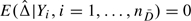

Observe that conditional on the control sample, the variance of is

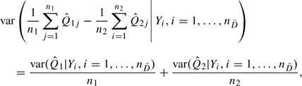(3.3)

which can be consistently estimated by , where denotes the sample variance. On the other hand, the unconditional variance of can be estimated by

(3.4)

As a result, the conditional test comparing the means of and is always more powerful than the unconditional test. This is corroborated by the highly significant results in the top row of Table 1 in Appendix A of the supplementary material, available at Biostatistics online.

According to Proposition 1, Q₁Q2⇔Y1Y2. Therefore, an alternative way to test H₀:Q₁Q₂ is to compare the distributions of Y₁ and Y₂. Standard 2-sample tests for comparing 2 groups, such as the t-test, Wilcoxon rank sum test, or permutation test, all can be used for this purpose. Tests based on raw marker measurements and percentile values have the same type-I error under the null hypothesis but different powers under alternative hypotheses. In the example, the test comparing means of Y₁ and Y₂ is highly significant (Table 1 in Appendix A of the supplementary material, available at Biostatistics online), reaching the same conclusion as the test for equal means of and , but this might not be true in other circumstances.

In summary, comparison of a marker's ability to differentiate 2 case groups from the same control group can be based on means of their percentile values Q₁ and Q₂. To construct a CI for E(Q₁) − E(Q₂), we need to use unconditional inference that incorporates variability in controls as well as cases. On the other hand, simply to perform a hypothesis test for equality of the distributions of Q₁ and Q₂, the conditional methods should be used because of their enhanced power.

3.2. Rank statistics

Section 3.1 dealt with comparisons of mean percentile values. However, when distributions of percentile values do not belong to the same location-scale family (as shown in Figures 1b and c), alternatives to mean differences may be considered. For example, we can use rank-based statistics such as the Wilcoxon rank sum test, which is often used for comparing 2 groups of independent observations. For the problem at hand, we need to acknowledge the correlation among s when applying the Wilcoxon rank sum test to them.

By analogy with methods in Section 3.1, we can apply the Wilcoxon rank sum test to and “unconditionally” or “conditional” on the control sample. In the former, the null hypothesis tested is 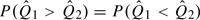, which holds if Q₁Q₂ according to Proposition 1. In the latter, the null hypothesis tested is , which holds for all sets of control samples if Q₁Q2. With the conditional testing, and are independent and the standard Wilcoxon rank sum test can be applied. For the unconditional test, the variance of the Wilcoxon rank sum test statistic can be estimated using the bootstrap.

In the ovarian cancer example, both the conditional and the unconditional Wilcoxon rank sum tests applied to suggest highly significant differences in the distributions of CA-125 percentile values between benign tumor cases and ovarian cancer cases (Table 1 in Appendix A of the supplementary material, available at Biostatistics online). Again, the conditional test is more powerful than the unconditional test since it does not involve variability in the control sample.

According to Proposition 1, we can also apply the Wilcoxon rank sum test to Y₁ and Y₂ to test the null hypothesis Q₁Q₂. Contrast the rank statistic based on Y₁ and Y₂ and that based on and . If the transformation from Y to does not change each observation's rank in the sample, then the rank-based statistic remains the same. This happens when F is modeled as a strictly monotone increasing function but does not necessarily happen when F is estimated nonparametrically because ties may be created during the empirical CDF transformation. The increase in the number of ties will potentially affect the value of the test statistic and reduce its variance. For example, in the ovarian cancer data, the Wilcoxon rank sum test statistic applied to Y₁ and Y₂ has a value of − 524 with a standard error 109.6, while the statistic applied to and has a value of − 437 with a standard error 90.9 when F is estimated empirically.

Note that if the nonparametric bootstrap is used for inference, the increase in ties during sampling with replacement can lead to underestimation of the variance. The severity of this problem depends on the sample size and the distribution of the percentile values. We found in limited simulation studies that for small sample size and good classification accuracy, applying the Wilcoxon rank sum test to with nonparametric bootstrap variance estimate led to anticonservative type-I error, especially when F is estimated empirically. A solution is to use the smoothed bootstrap (Silverman, 1986), (, SilvermanAndYoung1987). The idea is to simulate from smoothed distributions to avoid ties during resampling. There has been little systematic investigation about the choice of optimal bandwidth in this context. We explored several bandwidths in simulation studies and chose the bandwidth that covers around 40% of the total sample points in our data example. If variance estimation itself is not of interest, an alternative is to construct CIs based on percentiles of the nonparametric bootstrap distributions, an approach that turns out to be much less liberal than the Wald test based on nonparametric bootstrap variance estimates.

In summary, we can compare the discriminatory performance of a marker across different case groups using rank-based tests. We recommend (1) testing based on instead of Y because the former is more relevant to differences in diagnostic accuracy and (2) using the conditional rather than the unconditional test because the former can be performed with standard statistical software and is more powerful, whereas the latter calls for smoothed bootstrap for variance estimation without a sound theoretic basis for bandwidth selection.

3.3. Adjusting for covariates

Suppose the biomarker distribution in controls varies with a covariate X that can vary among cases, then the appropriate reference distribution should depend on X. We define the covariate-specific percentile value

(3.5)

where F(Y|X) is the CDF of the marker in the control population with covariate value X. In clinical medicine, for anthropometric measurements it is standard practice to calculate covariate-specific percentile values. For example, the percentiles of height for children are age and gender specific because these factors affect height in normal healthy children. Berres and others (2008) described methods to estimate covariate-specific diagnostic scores.

To compare women with benign tumors and women with ovarian cancer, we can evaluate covariate-specific percentile values for each case group and compare them using 2-sample test statistics. Is covariate adjustment important? The answer is “potentially yes.” Suppose, for example, that X is age and that in controls older age is associated with larger values of the biomarkers. If women with ovarian cancer tend to be older than women with benign tumors, one would observe a difference in discriminatory performance that is simply due to age. Using age-adjusted biomarker percentiles is a simple way to eliminate such confounding.

If X is discrete and there are relatively large numbers of controls per X category, a nonparametric approach to estimating F(Y|X) can be taken. Otherwise a parametric model is employed. For z = 1,2, let Q_zX(_zX) be the (estimated) covariate-specific percentile value for an observation in case group z. Let Δ = E(Q_1X) − E(Q_2X) and =_X−_X. When covariate X is discrete with K categories, let n_k and n_zk be the number of controls and the number of zth type of cases in the kth covariate category, k = 1,…,K.

THEOREM 3.2

Suppose , and . When X is discrete, suppose , n_1k/n₁→p_1k∈(0,1), and n_2k/n₂→p_2k∈(0,1). Then converges to a mean 0 normal random variable with variance σ², where

(3.6)

if F(Y|X) is modeled with the empirical CDF within the kth covariate category, where and the k superscript indicates cases and controls in covariate category k, and

(3.7)

if F(Y|X) is modeled parametrically, where Σ(θ) is the asymptotic variance of and we assume that Δ is differentiable with respect to θ and that ℱ = {F_θ(y|x):θ∈Θ} is a Donsker (1952) class.

To illustrate, we simulated a continuous covariate X for the ovarian cancer data. X is generated to be positively associated with both CA-125 and disease status, X∼N(μ,σ) where μ = 10×log{5×I(benign tumors)×I(log(CA-125) > 2.2) + 0.8×I(ovarian cancer) + 1.5×log(CA-125)} and σ = 4. Figure 2 shows the distribution of log(CA-125) ignoring covariate X and when X is equal to its first, second, and third quartiles in the whole sample. Observe that the distribution of log(CA-125) in controls varies with X. Moreover, the separations between controls and case groups differ with X.

Fig. 2.

Marginal and covariate-specific distributions of log(CA-125) in healthy women, women with benign ovarian tumors, and women with ovarian cancer.

We calculated the covariate-specific percentile values assuming normality of log(CA-125) in controls conditional on X. The mean is modeled as a cubic B-spline in X, with pre-chosen knots at the first 3 quartiles in the control sample. Figure 3 plots the distributions of the marginal and covariate-specific percentile values of CA-125 for women in the 2 case groups. It appears that adjusting for the covariate X reduces the separation between women with benign tumors and healthy women, while the separation between women with ovarian cancer and healthy women is unchanged. Indeed, the covariate-specific percentile values have an approximately uniform (0,100) distribution for women with benign tumors indicating that their distribution is the same as that for controls. Therefore, covariate adjustment appears to be desirable in this setting. After covariate adjustment, CA-125 picks up fewer benign tumor cases while maintaining its ability to identify ovarian cancer cases.

Fig. 3.

Marginal and covariate-adjusted distributions of estimated percentile values of CA-125 for women with benign ovarian tumors and women with ovarian cancer.

We now formally compare the 2 groups of cases with regard to their covariate-specific percentile values. All the unconditional tests described in Sections 3.1 and 3.2 can be applied. All tests suggest that CA-125 has significantly better discriminatory performance for identifying ovarian cancer compared to benign tumors (Table 2 in Appendix A of the supplementary material, available at Biostatistics online). In terms of estimation, we find that, as expected for benign tumors, _X is close to the uninformative marker value of 50 (_X=50.13). In the ovarian cancer group, _X=88.10 which is similar to the mean unadjusted percentile values (=90.17). The difference in the covariate-adjusted means is = − 37.96, with 95% CI ( − 57.76, − 18.16) based on the asymptotic variance and ( − 58.79, − 17.13) based on the bootstrap variance.

In summary, when the marker distribution in controls varies with a covariate that can vary among cases, covariate-specific percentile values can be calculated to eliminate potential confounding. The 2 groups of cases can then be compared using mean or rank-based statistics. This provides a covariate-adjusted comparison of the discriminatory capacity of the marker. See Janes and Pepe (2008a), (JanesAndPepe2008c) for a broad discussion of covariate adjustment.

4. COMPARING MARKERS

Next, consider the comparison of 2 markers with respect to their diagnostic accuracies. Two markers are measured on each of n_D cases and n controls. Let F_z,z = 1,2, be the distribution function for the zth marker in controls, and let Q_z(_z) denote the corresponding (estimated) case percentile value. Observe that each marker is standardized with respect to its own control reference distribution. Even though the raw marker values may be in different units, the transformation to percentile values put them on the same scale.

4.1. Using means

For each case, one can compare Q₁ and Q₂. If Q₁ tends to be larger than Q₂, then marker 1 is the better marker. Formally, let Δ = E(Q₁) − E(Q₂). The difference in sample means can serve as the basis of a test statistic =−.

In this 2-marker setting, correlation between the estimated percentile values comes from 2 sources: one due to subject-specific effects and the other due to estimation of the reference distributions. We need to acknowledge this correlation in making inference.

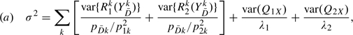
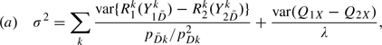
THEOREM 4.1

Suppose n_D/n→λ as n→∞, then converges to a mean 0 normal random variable with variance σ², where

(4.1)

if F_z is estimated with the empirical CDF, where Y_z and Y_zD are measurements of the zth marker for a control and a case, respectively, and R_z(Y_z)=P(Y_zD < Y_z) is the percentile value of the zth marker from a control in the corresponding case distribution (Delong and others, 1988), and

(4.2)

if F_z is modeled parametrically with parameter θ_z, where θ = (θ₁,θ₂), Σ(θ) is the asymptotic variance of , and we assume that Δ is differentiable with respect to θ

In practice, σ² can be estimated based on these formulas or by bootstrap resampling.

Observe that, for this 2-marker problem, conditional inference is no longer applicable. Even if the distributions of Q₁ and Q₂ are the same, the distributions of and conditional on the particular control sample will not necessarily be equal. Therefore, testing the null hypothesis that |{Yi,i=1,…,n}|{Yi,i=1,…,n} is not equivalent to testing the null hypothesis that Q₁Q₂.

The data set we use for illustration here is from the pancreatic cancer serum biomarker study (Wieand and others, 1989), which includes 90 cases and 51 controls. Serum samples from each patient were assayed for CA-19-9, a carbohydrate antigen, and CA-125, a cancer antigen.

Figure 4(a) shows the probability distributions of the markers. Also displayed are the distributions of the estimated case percentile values for each marker, with F_z estimated empirically in Figure 4(b), and under the assumption that Y is normally distributed after Box–Cox transformation in Figure 4(c). Clearly, the distribution of the percentile values for CA-19-9 is shifted to the right compared with CA-125, indicating that it is a better biomarker.

Fig. 4.

Distributions of log(CA-19-9) and log(CA-125) in controls and cases (a); distributions of the estimated case percentile values when control distributions are estimated empirically (b) or parametrically (c).

Next, consider the mean percentile values. When F_z is estimated empirically, =86.23 for CA-19-9, =70.70 for CA-125, and =15.53. The corresponding 95% CI for Δ is (4.34,26.73) using the asymptotic variance and similarly (4.37,26.70) using the bootstrap variance. When F_z is estimated parametrically, results are similar: =86.07, =71.09, and =14.97. The corresponding 95% CI for Δ is (3.80,26.15) using the asymptotic variance and (3.57,26.38) using the bootstrap variance. CA-19-9 performs significantly better than CA-125 for diagnosing pancreatic cancer (see also Table 2 in Appendix A of the supplementary material, available at Biostatistics online, for p-values).

In summary, to compare the diagnostic accuracy of 2 markers, we can use the controls to standardize the marker values in cases and compare the corresponding means. If n=∞, this is essentially a paired t-test. If n < ∞, the paired t-test needs to be modified to accommodate the additional variability in the estimated control marker distributions.

4.2. Using rank statistics

Rank-based tests provide another avenue to compare the distributions of percentile values. Due to their complicated correlation structure, standard variance formulas for rank-based test statistics no longer apply. The bootstrap method is used instead. Moreover, as discussed earlier, conditional tests are not applicable here. So only unconditional tests are considered.

PROPOSITION 2

Under H₀:Q₁Q₂, we have when F_z is estimated empirically.

PROPOSITION 3

Let U_j=_j−_j,j=1,…,n_D. Let T and S be the Wilcoxon signed rank test statistic and the Sign test statistic, respectively. Under H₀:Q₁Q₂, we have E(T) = (n_D + 1)/4 and E(S) = 1/2 when F_z is estimated empirically.

PROPOSITION 4

Let r_k be the rank of k, where

Let W = ∑_{k = 1}^n_Dr_k be the Wilcoxon rank sum test statistic. Then under H₀:Q₁Q₂, E(W) = n_D(2n_D + 1)/12 when F_z is estimated empirically.

We expect the results in Propositions 2–4 to hold asymptotically when F_z is estimated parametrically. In other words, under H₀:Q₁Q₂, the expectations of these rank-based test statistics applied to and are the same as that in the standard 2-sample setting (for W) and the paired-data setting (for T and S). Therefore, to test for equal discriminatory performance of 2 markers, we can apply the rank-based test statistics to and , bootstrapping the variance. Here, we face the same concerns about underestimation of the variance as in Section 3.2. Using the smoothed bootstrap for variance estimation or constructing CIs based on nonparametric bootstrap distributions seems to be a solution. Asymptotic distribution theory appears to be very challenging. Using a smoothed bootstrap with a bandwidth covering approximately 40% sample points, all rank-based tests suggest a highly significant difference between the 2 markers (Table 2 in Appendix A of the supplementary material, available at Biostatistics online).

4.3. Adjusting for covariates

We argued earlier that adjusting for covariates may be important when comparing 2 case groups. This is also potentially important when comparing 2 biomarkers. Suppose, for example, that biomarker values in the control group vary with study site in a multicenter study. Such might occur if collection or processing procedures differed across sites. If the site-specific control populations are pooled to form a reference set, the distribution of the case percentiles may be more diffuse than if the site-specific controls are used as the reference group (see the right side of Figure 5 for an example). Even if the case–control ratio is the same across study sites, biomarker performance can appear to be worse than it is by using a pooled reference set (Janes and Pepe, 2008b). Markers may differ with regard to this phenomenon. For example, processing techniques that vary across sites may affect one marker but not another. Differential covariate effects on reference distributions of biomarkers therefore can bias the comparison of markers unless proper adjustment is undertaken. The use of covariate-specific percentile values is a means to adjust for covariates and avoid this bias. Note that pertinent covariates may be different for different markers.

Fig. 5.

Marginal and covariate-specific distributions of log(CA-19-9) and log(CA-125) in controls and cases.

For z = 1,2, let Q_zX(_zX) be the (estimated) covariate-specific percentile value for the zth marker, Δ = E(Q_1X) − E(Q_2X) and =_X−_x. When X is discrete with K categories, let n_k and n_Dk be the numbers of controls and cases in the kth covariate category, k = 1,…,K. Again covariate adjustment is only relevant when the covariate is defined for both cases and controls.

THEOREM 4.2

Suppose as , and for a discrete covariate, , then converges to a mean 0 normal random variable with variance σ², where

(4.3)

if the covariate-specific reference distribution F(Y|X) is estimated empirically within each covariate category, where is the percentile value for a control using its covariate-specific case distribution as the reference for the zth marker in the kth covariate category, and

(4.4)

if F(Y|X) is modeled parametrically for marker z with parameter estimate θ_z, where θ = (θ₁,θ₂) and Σ(θ) is the asymptotic variance of . We assume that Δ is differentiable with respect to θ and that ℱ = {F_θ(y|x):θ∈Θ} is a Donsker class.

As shown in the supplementary material, available at Biostatistics online, Theorem 4 extends to the setting when different covariates are used to adjust different markers.

To illustrate, we simulate a discrete covariate X for the pancreatic cancer data. We set X to 1 for those with CA-125 above its median, and 0 otherwise. In total, 14 out of 51 (27.4%) controls and 57 out of 90 (63.3%) cases have X = 1. Figure 5 shows the probability distributions of log(CA-19-9) and log(CA-125) conditional on X.

For CA-19-9, the value of X does not have a dramatic influence on the reference control distribution, suggesting that covariate adjustment is not warranted. On the other hand, for CA-125, since the marker is positively associated with X and a higher percentage of cases have X = 1 compared with controls, the distribution for cases shifts to the right compared to the distribution for controls when data are pooled over X, even if there is not much difference between them conditional on X. In other words, X is a confounder for CA-125 but not for CA-19-9. Distributions of the covariate-specific percentile values for CA-19-9 (_X) and CA-125 (_X) in cases are shown in Figure 6. For CA-19-9, covariate adjustment does not affect the distribution of the case percentile values, whereas for CA-125, covariate adjustment removes the confounding effect of X and suggests performance that is poorer than its marginal performance.

Fig. 6.

Marginal and covariate-adjusted distributions of the estimated case percentile values of CA-19-9 and CA-125.

With F(Y|X) estimated empirically, we have _X=87.25 for CA-19-9, _X=53.85s for CA-125, and =33.40. The corresponding 95% CI for Δ is (20.04,46.76) using the asymptotic variance and (20.83,45.97) using the bootstrap variance. With F(Y|X) estimated parametrically under the assumption that Y is normally distributed after Box–Cox transformation within each covariate category, we find _X=87.09, _X=54.20, and =32.89. The corresponding 95% CIs for Δ are (18.97,46.81) and (20.38,45.40) using the asymptotic and bootstrap variances, respectively. See Table 2 in Appendix A of the supplementary material, available at Biostatistics online, for p-values based on mean and rank statistics. CA-19-9 appears to be a much better marker than CA-125 for identifying pancreatic cancer, especially after adjusting for the covariate.

5. RELATIONSHIPS WITH ROC ANALYSIS

Our approach to evaluating the capacity of a marker to distinguish cases from a reference set of controls is to use the control marker distribution to standardize marker values for cases. If these percentile values tend to be high for many cases, the marker's discriminatory capacity is good. We noted earlier that the approach is intuitive and is used in some applications (McIntosh and others, 2004). Interestingly, it is equivalent to ROC analysis, which plays a central role in biomarker evaluation (Baker, 2003), (Pepe, 2003). The equivalence has been noted previously (Pepe and Cai, 2004), (, PepeAndLongton2005). In particular, since the ROC curve, a plot of true-positive rate (TPR) = P(Y > c|D = 1) versus false-positive rate (FPR) = P(Y > c|D = 0), can be written as

(5.1)

where S = 1 − F, we see that the ROC curve is the CDF of 1 − F(Y) in cases. Thus, comparing case distributions of biomarker percentile values, Q = 100×F(Y), is entirely equivalent to comparing ROC curves. The representation of the distribution of Q in terms of the ROC curve provides further justification for using case percentile values as the unit of analysis in evaluating and comparing markers. Empirical ROC curves for the ovarian and pancreatic cancer data sets are shown in Figure 1 in Appendix A of the supplementary material, available at Biostatistics online.

Some of the procedures presented in Sections 3 and 4 are alternative representations of existing procedures for comparing ROC curves while some are new procedures. Using the fact that the mean of a random variable is equal to the area under its survival function, we see that the average of case percentile values can be represented in terms of the area under the ROC curve (AUC) (Bamber, 1975),

(5.2)

Thus, comparisons based on mean percentile values are equivalent to comparisons of AUCs, the classical approach to comparing ROC curves.

Hanley and Hajian-Tilaki (1997) represented the empirical AUC as the sample mean of case percentile values with F estimated empirically. The asymptotic results in Theorems 1(a) and 2(a) are results for empirical AUC differences that have been previously reported (Sukhatme and Beam, 1994), (, DelongEtal1988). However, their semiparametric counterparts in Theorems 1(b) and 2(b) have not. Li and others (1996) studied semiparametric estimation of the ROC curve when the case distribution is modeled parametrically and the control distribution is modeled empirically. We did the reverse in this paper using a flexible smooth form for the reference control distribution. The Box–Cox family has precedent in modeling reference distributions for anthropometric measures (Cole, 1990). Returning to the asymptotic results in Theorems 1(a) and 2(a), in contrast to Sukhatme and Beam (1994) and similar to Hanley and Hajian-Tilaki (1997), we reparameterized the variances in terms of percentile values in this report, which we feel is a more intuitive way to understand the components of the variance.

A problem with comparing the diagnostic accuracy of 2 tests using AUC is lack of power to detect differences in ROC curves when they have the same area under the curve. As pointed out by Swets (1986), ROC curves are typically asymmetric, and 2 ROC curves with different asymmetries might cross each other but have the same AUC. Venkatraman and Begg (1996) developed a permutation test procedure to compare 2 ROC curves with paired data. Extension of the permutation test to the setting of continuous unpaired data was also proposed (Venkatraman, 2000). Extension to comparisons among more than 2 tests, however, might be computationally intensive.

The rank statistics described in Sections 3.2 and 4.2 provide an alternative solution to distinguishing between curves with the same AUCs. They have power to reject H₀:Q₁Q₂ when E(Q₁) = E(Q₂) but P(Q₁ > Q₂)≠P(Q₁ < Q₂). These can be interpreted as new ROC analysis techniques. Yet, their interpretation as rank statistics to compare distributions of standardized biomarkers in cases is equally valid and may be preferred by some. The generalization to comparing distributions of multiple standardized biomarkers is also tenable (Cuzick, 1985), (, KruskalAndWallis1952).

Nakas and others (2003) proposed comparing markers using functions of case percentile values. Their statistic is a nonstandard ROC summary index, namely, the 1-sample Anderson–Darling goodness-of-fit test statistic for the hypothesis that F(Y) in cases is uniformly distributed. This approach is in fact a special case within our proposed framework of comparing standardized marker distributions. In our opinion, applying a modified 2-sample version of the corresponding test directly to the standardized marker values is conceptually more straightforward.

The concept of covariate adjustment has only recently been developed for ROC analysis. The use of the covariate-specific percentiles provides a simple intuitive and easily implemented approach to adjust for covariates. Interestingly, arguments similar to (5.1) prove that the distribution of the covariate-specific case placement values, 1 − Q/100, is the covariate-adjusted ROC curve, 𝒜ROC(t), proposed by Janes and Pepe (2008a), Janes and Pepe (2008b), Janes and Pepe (2008c). Thus, our methods for comparing distributions of the covariate-specific percentiles can be interpreted as methods to compare the 𝒜ROC curves. Formal methods for comparing the 𝒜ROC curves have not been available heretofore. Our methods based on mean covariate-specific percentiles compare areas under the 𝒜ROC curves while methods based on ranks provide an alternative approach.

In this paper, we focus primarily on comparing the ROC curve across the entire range of FPRs∈(0,1). In practice, one might focus on a part of the ROC curve that is of primary interest. For example, in screening studies, FPRs must be kept very low and so the ROC curve over a restricted range of FPR may be of interest. The percentile value framework is well suited to evaluations over restricted regions. If FPR is fixed at u, as we have shown, comparing ROC(u) can be achieved by comparing between samples. If FPR in the range (0,u) is of interest, the partial AUC defined as pAUC(u) = ∫₀^uROC(t)dt has been proposed as the basis for marker comparisons (McClish, 1989). The empirical estimator written in terms of percentile values is

where the empirical is used to calculate _i. This result follows by noting that

Returning now to the ovarian cancer and pancreatic cancer examples, suppose we are interested in comparisons based on ROC(u) and pAUC(u) for u = 0.20. We model the reference distributions parametrically and rely on the resampling variance for inference. In the ovarian cancer example, before covariate adjustment, ₁(u)=0.5, ₂(u)=0.86, with a difference of − 0.36(95%CI = ( − 0.61, − 0.12)); ₁(u)=0.07, 2(u)=0.17, with a difference of − 0.09(95%CI = ( − 0.14, − 0.05)). After covariate adjustment, ₁(u)=0.29, ₂(u)=0.83, with a difference of − 0.54(95%CI = ( − 0.80, − 0.29)); ₁(u)=0.04, 2(u)=0.16, with a difference of − 0.12(95%CI = ( − 0.16, − 0.07)). In the pancreatic cancer example, before covariate adjustment, ₁(u)=0.79, ₂(u)=0.49, with a difference of 0.3 (95% CI = (0.11, 0.49)); ₁(u)=0.14, ₂(u)=0.06, with a difference of 0.08 (95% CI = (0.05, 0.12)). After covariate adjustment, ₁(u)=0.83, ₂(u)=0.3, with a difference of 0.53 (95% CI = (0.36, 0.71)); ₁(u)=0.15, ₂(u)=0.03, with a difference of 0.12 (95% CI = (0.08, 0.15)). Comparisons based on points and partial areas under the curve agree with those based on the whole curve.

6. CONCLUDING REMARKS

Standardizing a biomarker or diagnostic test to a reference population of controls is not an entirely new concept. However, it is not yet a standard approach to biomarker evaluation. We suspect 2 reasons. First, ROC analysis has become the standard of practice (Baker, 2003), and second, formal methods have not been available for statistical inference that properly take account of sampling variability in the reference distribution. This paper provides remedies by providing methods for statistical inference and by noting that the approach is interchangeable with ROC analysis. We feel that the approach should be encouraged because of its conceptual simplicity.

The approach also opens up new avenues for evaluating biomarkers and diagnostic tests. For example, covariate adjustment is naturally handled within this framework. We illustrated that covariate adjustment can be important when comparing biomarkers or for comparing the performance of a biomarker in 2 populations. Pepe and Cai (2004) and Cai (2004) already showed how ROC regression can be accomplished by performing regression analysis of case standardized marker values. In the context of evaluating biomarkers for event time outcomes, one might use the risk set at time t to standardize the biomarker for the subject that fails at t (the case). Interestingly, it can be shown that the distribution of such standardized values is closely related to the time-dependent ROC curves developed by Heagerty and Zheng (2005). We hope that the methods presented here will encourage use of the percentile value standardized approach in practice and encourage further development of new techniques for biomarker evaluation.

FUNDING

National Institutes of Health (GM-54438 and CA-86368); Pacific Ovarian Cancer Research Consortium/SPORE in Ovarian Cancer (P50 CA83636, N.U.).

References

- Baker SG. The central role of receiver operating characteristic (ROC) curves in evaluating tests for the early detection of cancer. Journal of the National Cancer Institute. 2003;95:511–515. doi: 10.1093/jnci/95.7.511. [DOI] [PubMed] [Google Scholar]
- Bamber D. The area above the ordinal dominance graph and the area below the receiver operating characteristic graph. Journal of Mathematical Psychology. 1975;12:387–415. [Google Scholar]
- Berres M, Zehnder A, Blasi S, Monsch AU. Evaluation of diagnostic scores with adjustment for covariates. Statistics in Medicine. 2008;27:1777–1790. doi: 10.1002/sim.3120. [DOI] [PubMed] [Google Scholar]
- Cai T. Semi-parametric ROC regression analysis with placement values. Biostatistics. 2004;5:45–60. doi: 10.1093/biostatistics/5.1.45. [DOI] [PubMed] [Google Scholar]
- Cole TJ. The LMS method for constructing normalized growth standards. European Journal of Clinical Nutrition. 1990;44:45–60. [PubMed] [Google Scholar]
- Cuzick J. A Wilcoxon-type test for trend. Statistics in Medicine. 1985;4:87–90. doi: 10.1002/sim.4780040112. [DOI] [PubMed] [Google Scholar]
- Delong ER, Delong DM, Clarke-Pearson DL. Comparing the areas under two or more correlated receiver operating characteristic curves: a nonparametric approach. Biometrics. 1988;44:837–845. [PubMed] [Google Scholar]
- Donsker MD. Justification and extension of Doob's heuristic approach to the Kolmogorov-Smirnov theorems. Annals of Mathematical Statistics. 1952;23:277–281. [Google Scholar]
- Frischancho AR. Anthropometric Standards for the Assessment of Growth and Nutritional Status. Ann Arbor, MI: University of Michigan Press; 1990. [Google Scholar]
- Hanley JA, Hajian-Tilaki KO. Sampling variability of nonparametric estimate of the areas under receiver operating characteristic curves: an update. Vol. 4. Academic Radiology; 1997. pp. 49–58. [DOI] [PubMed] [Google Scholar]
- Heagerty PJ, Zheng Y. Survival model predictive accuracy and ROC curves. Biometrics. 2005;61:92–105. doi: 10.1111/j.0006-341X.2005.030814.x. [DOI] [PubMed] [Google Scholar]
- Janes H, Pepe MS. Adjusting for covariate effects on classification accuracy using the covariate-adjusted receiver operating characteristic curve. UW Biostatistics Working Paper Series. 2008a doi: 10.1093/biomet/asp002. Working Paper 283. [DOI] [PMC free article] [PubMed] [Google Scholar]
- Janes H, Pepe MS. Adjusting for covariates in studies of diagnostic, screening, or prognostic markers: an old concept in a new setting. American Journal of Epidemiology. 2008b;168:89–97. doi: 10.1093/aje/kwn099. [DOI] [PubMed] [Google Scholar]
- Janes H, Pepe MS. Matching in studies of classification accuracy: implications for bias, efficiency, and assessment of incremental value. Biometrics. 2008c;64:1–9. doi: 10.1111/j.1541-0420.2007.00823.x. [DOI] [PubMed] [Google Scholar]
- Kruskal WH, Wallis WA. Use of ranks in one-criterion variance analysis. Journal of the American Statistical Association. 1952;47:583–621. [Google Scholar]
- Li G, Tiwari RC, Wells MT. Quantile comparison functions in two-sample problems, with application to comparisons of diagnostic markers. Journal of the American Statistical Association. 1996;91:689–698. [Google Scholar]
- McClish DK. Analyzing a portion of the ROC curve. Medical Decision Making. 1989;9:190–195. doi: 10.1177/0272989X8900900307. [DOI] [PubMed] [Google Scholar]
- McIntosh MW, Drescher C, Karlan B, Scholler N, Urban N, Hellstrom KE, Hellstrom I. Combining CA 125 and SMR serum markers for diagnosis and early detection of ovarian carcinoma. Gynecologic Oncology. 2004;95:9–15. doi: 10.1016/j.ygyno.2004.07.039. [DOI] [PMC free article] [PubMed] [Google Scholar]
- Nakas C, Yiannoutsos CT, Bosch RJ, Moyssiadis C. Assessment of diagnostic markers by goodness-of-fit tests. Statistics in Medicine. 2003;22:2503–2513. doi: 10.1002/sim.1464. [DOI] [PubMed] [Google Scholar]
- Pepe MS. The Statistical Evaluation of Medical Tests for Classification and Prediction. Oxford: Oxford University Press; 2003. [Google Scholar]
- Pepe MS, Cai T. The analysis of placement values for evaluating discriminatory measures. Biometrics. 2004;60:528–535. doi: 10.1111/j.0006-341X.2004.00200.x. [DOI] [PubMed] [Google Scholar]
- Pepe MS, Longton GM. Standardizing markers to evaluate and compare their performances. Epidemiology. 2005;16:598–603. doi: 10.1097/01.ede.0000173041.03470.8b. [DOI] [PubMed] [Google Scholar]
- Silverman BW. Density Estimation for Statistics and Data Analysis. London: Chapman and Hall; 1986. [Google Scholar]
- Silverman BW, Young GA. The bootstrap: to smooth or not to smooth? Biometrika. 1987;74:469–479. [Google Scholar]
- Sukhatme S, Beam CA. Stratification in nonparametric ROC studies. Biometrics. 1994;50:149–163. [PubMed] [Google Scholar]
- Swets JA. Form of empirical ROC's in discrimination and diagnosis tasks: implications of theory and measurement of performance. Psychological Bulletin. 1986;99:181–198. [PubMed] [Google Scholar]
- Venkatraman ES. A permutation test to compare receiver operating characteristic curves. Biometrics. 2000;56:1134–1138. doi: 10.1111/j.0006-341x.2000.01134.x. [DOI] [PubMed] [Google Scholar]
- Venkatraman ES, Begg CB. A distribution-free procedure for comparing receiver operating characteristic curves from a paired experiment. Biometrika. 1996;83:835–848. [Google Scholar]
- Wieand S, Gail MH, James BR, James KL. A family of nonparametric statistics for comparing diagnostic markers with paired or unpaired data. Biometrika. 1989;76:585–592. [Google Scholar]
Associated Data
This section collects any data citations, data availability statements, or supplementary materials included in this article.