Uncovering the rules for protein–protein interactions from yeast genomic data

Abstract

Identifying protein–protein interactions is crucial for understanding cellular functions. Genomic data provides opportunities and challenges in identifying these interactions. We uncover the rules for predicting protein–protein interactions using a frequent pattern tree (FPT) approach modified to generate a minimum set of rules (mFPT), with rule attributes constructed from the interaction features of the yeast genomic data. The mFPT prediction accuracy is benchmarked against other commonly used methods such as Bayesian networks and logistic regressions under various statistical measures. Our study indicates that mFPT outranks other methods in predicting the protein–protein interactions for the database used. We predict a new protein–protein interaction complex whose biological function is related to premRNA splicing and new protein–protein interactions within existing complexes based on the rules generated. Our method is general and can be used to discover the underlying rules for protein–protein interactions, genomic interactions, structure-function relationships, and other fields of research.

Protein–protein interactions are essential for the formation of cellular networks. Identification of these interactions is crucial for the understanding of underlying cell functions and regulatory mechanisms. Some protein interactions can play important roles in many cellular processes (1, 2). In recent years, with the development of experimental technologies in genetics, genomes, expressions, and applications of high-throughput approaches, data about protein–protein interactions have been accumulated rapidly (3). The current methods of finding protein–protein interactions can be divided into several categories : biological methods such as Yeast Two Hybrid (Y2H) (4, 5) and Tandem Affinity Purification (TAP) (6); computational methods such as Phylogentic Profile (7) and the correlated domain signature method (8); and integrative methods (9). Issues concerning the methods remain: Most are applied only to a limited set of protein pairs and do not cover all of the possible interactions; and the overlap between the predictions of different methods is often small (9). One needs to integrate evidence from different sources when evaluating protein–protein interactions. Some recent efforts have been made (e.g., refs. 1 and 10) trying to combine several attributes into one integrated predictor. These attributes can be from either predictions of other methods or from different data sources. Widely used methods feature integration, including Bayesian approaches (1, 11), decision trees (2), support vector machines (12), and neural networks (1, 13).

In our study, we employ an adapted frequent pattern tree (see Table S1) method (14, 15) to generate a minimum set of rules (FPT) and apply it to integrate protein–protein features from multiple data sources. Different protein–protein interactions form patterns in the spaces expanded by their features. Consequently, the number of possible patterns grows combinatorially with the number of features. For a given database, the advantage of FPT is that it exhaustively searches for interactive patterns among all possible components up to a specified minimum number of appearances within the database–support level. The support controls the amount of the statistical robustness required to make our statistical predictions. In particular, when the support is set to be 1, FPT guarantees all interaction patterns within the development database to be found, including those rarely occurring ones often missed by other statistical methods. Our objective is to predict the pairwise protein–protein interactions given their features gathered from different sources. FPT patterns can be considered as rules with attributes constructed by the protein interaction features. We build all possible rules to predict protein interactions in the form of: if feature-1 and feature-2, etc., then interaction is expected.

False-positives can occur due to the data noise from unreliable experiments. Although not within the scope of our current study, FPT can also be applied to multibody interactions. One practical issue of using FPT is that rules generated by FPT largely correlate or overlap with each other. We adopted the FPT algorithm to generate a minimum number of rules (mFPT) without losing detection accuracy.

The mFPT method can extract significant rare patterns from large amounts of data. mFPT provides a powerful method of data mining for discovering underlying rules and making predictions. It can be used for scientific and engineering explorations such as bioinformatics, drug discovery, chemometrics, engineering design and quality control, and environmental control; industrial applications such as fraud detection and risk in banking and insurance; government administration such as the IRS, health care, and credit bureaus; and business and management applications such as database marketing, internet shopping, and customer relationship management (16).

Our study is prompted by an earlier integrated Bayesian approach to predict protein interactions (1). The protein features considered include mRNA expression, biological function, essentiality, and experimental data. Later on, the list of genomic features is expanded to 16, and assembled based on both single-protein and protein-pair features derived from a wide range of physical, genetic, contextual, and evolutionary properties of yeast genes.

For prediction and validation of the protein complexes, a standard dataset is created upon which our comparative studies with other statistical methods is based. MIPS (17) (Munich Information Center for Protein Sequences) complexes catalog were used as the positives (proteins within the same complex); a negative gold-standard is harder to define, but essential for successful training, so lists of proteins in separate subcellular compartments were collected as negatives (proteins do not interact) (13). The mFPT approach is used to train data and predict interactions based on their genomic features. Hence, our study, to be precise, is to predict whether 2 proteins are in the same complex, not whether they necessarily had direct physical contact. We validate the predicted results against actual results for the holdout sample to evaluate the prediction accuracy with several statistical measures and find that mFPT outperforms other data mining methods in predicting the protein–protein interactions. Rules for predicting protein–protein interactions are built consequently as the results of frequent patterns. Further, we predict and analyze a new protein–protein interaction complex with the rules obtained.

Results and Discussions

Rules of Protein–protein Interactions.

Genomic features for our computation include Essentiality data, Functional similarity data from MIPS and from Gene Ontology (GO) databases, mRNA expression data (1), and 12 other features.

First, we consider only the 5 most important genomic features. The input database for mFPT is organized in the same way as for FPT:

In Table 1, each line represents a protein pair, and each column represents one of the genomic features, denoting essentiality (ranging from 1 to 4), mRNA coexpression (13) (ranging from 5 to 24,), MIPS functional similarity (ranging from 25 to 30), GO functional similarity (ranging from 31 to 36), and experimental interacting datasets (ranging from 37 to 52); the last column represents whether the protein pairs interact, with 95 for positive and 94 for negative. We then divide data samples to 2 training (70%) and testing (30%) files.

Table 1.

Input format of FPT

Ess	mRNA	MIPS	GO	Expe	Interaction
4	9	28	35	51	95
3	7	28	35	51	95
4	6	25	35	51	95
2	13	29	36	52	94

Ess, essentiality; Expe, experiment.

We execute the mFPT algorithm with following steps:

• Run FPT once, produce a complete set of patterns.

• Sort these rules according to their performances. (Here we use the product of hit-rate and square root of number of hits by the rule.)

• Select the best rule. (We choose highest hit-rate above support level.)

• Remove the samples hit by this rule, go to step 1 and run FPT again.

mFPT arithmetic prescribes that the lower the minimum support is, the more accurate the rules are predicted. Here, we choose the minimum support as 1, the minimum hit rate as 0.5, below which considered to be insignificant rules.

After almost 50 loops, we obtain 53 rules.

Here, we choose top 10 rules to explain in Table 2:

Table 2.

Rules of FPT

Hit-rate	Support	Features
0.963	658	35, 28, 8
0.902	679	35, 28, 9
0.981	369	35, 28, 7
0.813	569	4, 35, 28, 10
0.854	391	28, 48
0.909	209	48, 26
0.980	151	34, 41
0.562	695	52, 4, 35, 11, 28
0.751	225	27, 48
1.000	78	52, 35, 28, 6

The meaning of category values are as follows: 1, both proteins are essential; 2, one is essential, another is not; 3, both are not essential; 4, not found in essentiality database; 5–23, Pearson correlations for each protein pair, and the smaller the category value is, the bigger correlation is; 24, not found in mRNA coexpression database; 25–29, MIPS value, and Mips increase with category values increased; 30, not found in MIPS database; 31–35, GO value, and GO increase with category values increased; 36, not found in GO database.

In Table 2, the first column represents the hit-rate (ratio of positives over positives plus negatives) of the corresponding patterns, and the second column expresses the number of hits (positive + negative). The rule 1 (first line) states that protein pair possessing higher coexpression level, lower MIPS and GO values, has a higher probability of interaction, consistent with intuitions. Rules 2, 3, 4, 8, and 10 are similar to rule 1 but differ in coexpression levels and experimental interaction indication. Rules 5, 6, and 9 state that higher MIPS (differ in their MIPS values with each other) and experimental interactions lead to higher hit. Rule 7 states that higher Go values and experimental indication leads to higher chance of the pair interaction.

Evaluations of Results with KS and ROC.

We predict protein–protein interactions in training and testing datasets using the 53 rules. We evaluated the number of true/false positives predictions in the testing set. We calculated the Kolmogorov and Sminov Statistics (KS) values and Receiving Operator Characteristic (ROC). Both KS and ROC give the quantitative measure of how good the discrimination is in identifying the protein–protein interactions (SI Text).

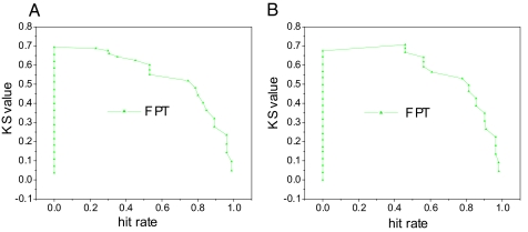
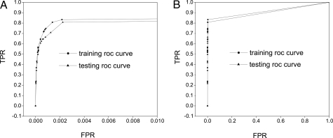
The KS values are >50% with a 0–80% hit rate in training samples, and KS values are >50% with a 0–60% hit rate in testing samples as shown in Fig. 1. This indicates the robust separation power of the protein–protein interactions with only a few of the most important rules. This is also reflected on the ROC curve with sharp increase of sensitivity (TPR: the ratio of true positives with respect to the sum of true positives and false negatives) with respect to specificity (FPR: the ratio of true negatives with respect to the sum of true negatives and false positives) in both training and testing samples as shown in Fig. 2.

Fig. 1.

FPT KS curve of training (A) and testing (B) samples.

Fig. 2.

FPT ROC curves (A and B) for different scales. Red curves represent training samples, and green curves represent testing samples.

Comparison with Different Methods.

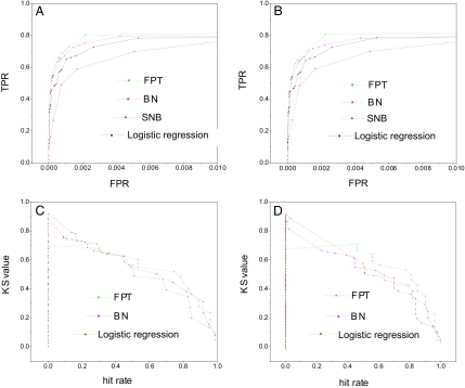
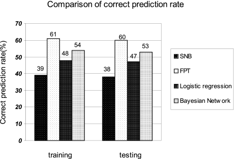
For the purpose of benchmarking, we perform the protein–protein interaction prediction using the Bayesian network (BN) approach (see Figs. S1 and S2) (18, 19), the logistic regression method, and the simple naive Bayesian classifier (SNB) used in (1). Fig. 3 A and B shows the comparisons of the results of ROC curve for different methods for both training and testing samples. From these graphs, we can see that the mFPT and the Bayesian network perform better because their ROC curves climb more rapidly toward the upper left corner (high sensitivity versus specificity), and the mFPT approach is mildly better than Bayesian network. Fig. 3 C and D shows the KS value comparisons. In a wide range of hit rate ranging from 40% to 100%, the mFPT outperforms other methods with higher discrimination power. Fig. 4 shows the comparisons of the correct prediction rate (equals sensitivity in ROC curve) when hit rate is 0.5. mFPT performs the best.

Fig. 3.

ROC curve and KS value comparisons for 4 methods. (A and B) ROC curve comparisons of the training (A) and testing (B) samples for 4 methods. (C and D) KS value comparisons of the training (C) and testing (D) samples for 4 methods.

Fig. 4.

Comparisons of correct prediction rate for 4 methods for both training and testing samples

Results of Adding New Features.

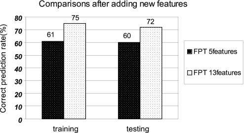
To further test the performance of mFPT, we added more features to predict. We integrated 8 more features from different sources of data (including EXP, Mes, APA, REG, PGP, GNN, ROS, and INT, for a total of 5 + 8 = 13 features) from the total 12 features to perform the mFPT data mining. We change the minimum support to 3 for the sake of computational time. We compare the correct predictions of 5 features and 13 features (see Fig. 5). In SI Text, we show the ROC curve and the KS value comparisons of mFPT with 5 features and 13 features, respectively (see Figs S3 and S4). From the results, we can see that integrating 13 features perform better than 5 features alone.

Fig. 5.

Comparisons of correct prediction rate for 5 features and 13 features with both training and testing data samples

We also compare the mFPT method with other data mining methods for 13 features (see Fig. S5). We found that mFPT is consistently better in the quantitative statistical measures ROC and KS of discriminating interactions. Fig. S6 in the supplement shows that mFPT predicts more accurately. This supports our conclusion that mFPT is the best predictor of all of the data mining methods included.

Predicting Protein–Protein Interactions in Existing Complex.

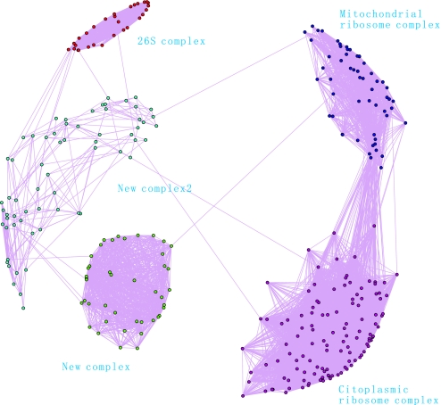
We obtain the network connection graph of protein interactions based on our mFPT predicted results using the pajek graphic software (20). By analyzing the network connection graph, we recognize some large complexes. For example, with 53 rules we predicted 15,222 pairs of protein interactions with 1,991 nodes when we integrate 5 feature values to predict results using mFPT. The network structure can be further reduced when we set certain minimum link values as thresholds. So, we can acquire 1 network with 316 nodes when the value of links is larger than 25.

From Fig. 6, we see 4 obvious complexes, including cytoplasmic ribosome, 26S proteasome, mitochondrial ribosome, and a new predicted one for premRNA splicing.

Fig. 6.

Predicted complex.

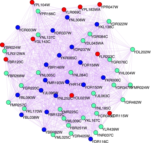
Mitochondrial ribosome(MR) is one of the largest complexes in our predicted network. Fig. 7 shows the network of mitochondrial ribosome complex in more detail. Our predictive results replicated well the MR proteins in the Saccharomyces Genome Database (www.yeastgenome.org). From Fig. 7 and Table S2, we can see that mFPT and SNB methods all predict some MR proteins and some related proteins; however, there are many other MR proteins that the mFPT method predicts but SNB does not. In Fig. 7, blue nodes represent proteins that mFPT and SNB both predict; cyan and red nodes represent proteins mFPT predicts but SNB does not. Most of the cyan nodes are Mitochondrial ribosomal proteins(MRPs) (21) (details in Table S2). Mitochondrial ribosomal proteins (MRPs) are the counterparts in that organelle to the cytoplasmic ribosomal proteins in the host (22). The function of mitochondrial (mt) ribosomes is the biosynthesis of a small number of proteins encoded by the mt DNA. Direct links to the functions of MRPs have been studied only at a rudimentary level (23). It has been suggested that mt ribosomes are more or less associated with the inner side of the mt inner membrane (24).

Fig. 7.

Mitochondrial ribosome complex.

Red nodes represent 10 proteins including YBR024W, YBR120C, YDR115W, YGL143C, YLR069C, YLR203C, YOL023W, YPL104W, YPL183WA, and YPR047W. They do not belong to MR proteins but are associated with MR proteins.

YLR069C(MEF1) is a translation elongation factor and should be transiently associated with the MR. YBR024W is a protein anchored to the mitochondrial inner membrane (25). YBR120C is a protein required for translation of the mitochondrial COB mRNA. YDR115W is putative mitochondrial ribosomal protein of the large subunit. It is similar to E. coli L34 ribosomal protein, as are most mitochondrial ribosomal proteins. YGL143C(MRF1) is a Mitochondrial polypeptide chain release factor, related to mitochondrial translation. YOL023W(MSS51) is a Mitochondrial translation initiation factor, which is associated with the MR. YLR203C Nuclear encoded protein required for translation of COX1 mRNA. YPL104W is Mitochondrial aspartyl-tRNA synthetase. YPL183WA is a homolog of the prokaryotic ribosomal protein L36, likely to be a mitochondrial ribosomal protein coded in the nuclear genome (22). Therefore, our predictions for these newly added proteins as mitochondrial ribosomal proteins are consistent with their biological functions.

In the same way, we can see that mFPT predict more proteins than SNB for 26S proteasome complex (26) and cytoplasmic ribosome complex (27, 28) from Tables S3 and S4 and Figs. S7 and S8 (blue nodes represent proteins that mFPT and SNB both predict, cyan nodes represent proteins that mFPT predicts while SNB does not). For 26S proteasome complex, mFPT predicts 29 proteins more than SNB's 13 proteins, and database search tells us that these newly predicted proteins all belong to 26S proteasome or 20S proteansome, which are associated with 26S proteansome.

Predicting New Protein–Protein Interaction Complex.

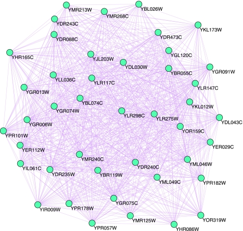
More importantly, there is another large complex in the lower left corner of Fig. 6, which we magnify in Fig. 8(see Table S5). This new complex includes 43 proteins. After searching through the SGD(Saccharomyces Genome Database) we found that these 43 proteins belong to 4 categories. They are Sm proteins, Sm-like proteins, snRNAs (U1, U2, U4, and U5), and other proteins related to snRNAs or premRNA processing.

Fig. 8.

New complex.

SnRNP proteins are involved in a wide variety of functions, including premRNA splicing (29, 30). The Sm protein was characterized by a domain present in a group of 8 small proteins (alternatively spliced products B, B′, D1, D2, D3, E, F, and G) that associated with 4 snRNAs, including U1, U2, U4, and U5. Sm-like proteins also encode proteins containing Sm domains and are thus named LSM (Like SM) proteins (29). And other proteins apart from these kinds are also related to the splicing of premRNA.

YBL026W and YER112W are Sm-like proteins. YER029C is a Core Sm protein Sm B, YGR074W is a Core Sm protein Sm D1, YLR147C is a Core Sm protein Sm D3, and YLR275W is a Core Sm protein Sm D2. YOR159C is a Core Sm protein Sm E, and YPR182W is a Core Sm protein Sm F. YBR055C, YDL030W, YDL043C, YMR268C, YDR473C, YPR178W, YML046W, YDR243C, YGL120C, YGR006W, YGR075C, YGR091W, YHR165C, YJL203W, YKL012W, YLL036C, and YDR235W are premRNA processing proteins. YBR119W, YLR298C, YGR013W, YIL061C, YDR240C, and YHR086W are components of U1 snRNP required for mRNA splicing (31). YIR009W, YOR319W, YML049C, and YMR240C are components of U2 snRNP, or U2-snRNP associated splicing factors involved in splicing. YBL074C and YKL173W are components of U5 snRNP, splicing premRNA protein. Others (including YMR213W, YLR117C, YMR125W, YPR101W, YDR088C, and YPR057W) are involved in mRNA splicing, or required for premRNA splicing (32).

Therefore, we can conclude that what we found is a new function complex related to premRNA splicing. And these comparison results with SGD further support the predicting power of mFPT method.

For the sparse structure in the left middle of our prediction graph (Fig. 6), we found that some components belong to RNA polymerase, and we do not have enough evidence to prove these proteins should be put together. Considering the numbers of interactions are lower in these structure, it seems that they may form a weakly connected complex.

Methods

Several studies have been carried out to search for individual features contained in the genomic datasets that are useful for protein interaction prediction. However, each genomic feature, by itself, is only a weak predictor of protein interactions. Therefore, predictions can be improved by integrating different genomic features (13).

Our study is motivated by an earlier integrated Bayesian approach to predict protein interaction (1). The various protein features considered include mRNA expression, biological function, essentiality, and experiment data. In a later study, the list of genomic features is expanded to 16 that are assembled based on both single and protein pair features, which are derived from a wide range of physical, genetic, contextual, and evolutionary properties of yeast genes.

For the validation and prediction of protein complexes, a reference dataset was created serving as gold-standards of positives (proteins that are in the same complex) and negatives (proteins that do not interact) (1). The Munich Information Center for Protein Sequences (MIPS) (17) complexes catalog was used as the gold-standard for positives. A negative gold-standard is harder to define, but essential for successful training. The negatives were collected from the lists of proteins in separate subcellular compartments (13).

We use the FPT approach to train data and predict interactions based on their gold-standard data and their genomic features. Hence, our goal, precisely defined, is to predict whether 2 proteins are in the same complex, not whether they necessarily had direct physical contact.

We can assess performance of FPT by comparing predicting results against samples of known positives and negatives (“gold-standards”). We can further on make new predictions.

Method of Frequent-Pattern Mining.

First, we examine Frequent-pattern mining (14, 15). Let I = A₁, A₂, …, A_m be a set of items, and a transaction database DB = T₁,T₂, …,T_n, where T_i (i = 1 … n) is a transaction that contains a set of items in I. The support (or occurrence frequency) of a pattern Q, where Q is a set of items, is the number of transactions containing Q in DB. Pattern Q is frequent if Q's support is no less than a predefined minimum support threshold, ξ. Given a transaction database DB and a minimum support threshold ξ, the problem of finding the complete set of frequent patterns is called the frequent-pattern mining problem (14, 15).

Mining frequent patterns in transaction databases has been a popular subject of study in data mining. Most studies on frequent pattern mining adopt the A priori algorithm (33). The bottleneck associated with this method is the huge candidate sets and multiple scans of the entire database with huge computational costs.

The FPT method discovers frequent patterns in transactional databases by FP-growth arithmetic. FP-growth (15) first performs a frequent item-based databases projection when the database is large and then constructs a compact data structure, called FP-tree, which is condensed but complete for frequent pattern mining. In this way, problem of mining a database is transformed into that of mining one compact tree. Compared with some representative frequent-pattern mining methods for data mining, the FPT approach has several advantages: It alleviates the multiscan problem and improves the candidate pattern generation; it is faster than A priori and outperforms the tree projection algorithm (34, 35) and it performs well especially when the dataset contain many patterns or when the frequent patterns are long (14, 15).

A frequent-pattern tree (or FP-tree in short) is a tree structure and it can be designed as follows.

1. It consists of 1 root labeled as “null,” a set of item-prefix subtrees as the children of the root, and a frequent-item-header table.

2. Each node in the item-prefix subtree consists of 3 fields: item-name, count, and node-link, where item-name registers which item this node represents, count registers the number of transactions represented by the portion of the path reaching this node, and node-link links to the next node in the FP-tree carrying the same item-name, or null if there is none.

3. Each entry in the frequent-item-header table consists of 2 fields, (i) item name and (ii) head of node link (a pointer pointing to the first node in the FP-tree carrying the item name).

According to the design principle, after scanning all of the transactions, the FP-tree could be constructed. First, a scan of DB derives a list of frequent items, such as (F:4), (C:4), (A:3), (B:3), (M:3) (here F, C, A, B, and M represent items, and the numbers after the colons indicate the support), in which items are ordered in frequency-descending order. Second, the root of a tree is created and labeled with “null.”

To facilitate tree traversal, an item header table is built in which each item points to its first occurrence in the tree via a node-link. Nodes with the same item-name are linked in sequence via such node-links. And an example of mFPT method's detailed designing process is shown in SI Text.

Conclusions

We have applied a mFPT approach to predict protein interactions integrating different sources of data and genomic features. mFPT outperforms other data mining methods included. We acquire reliable predicting results, see better correspondence with SGD. We also predict some new interactions within the existing complex and a new functional protein–protein interaction complex for premRNA splicing. With the addition of more genome features, our method can achieve greater performance. It is anticipated that this approach could be used to find protein interactions in other organisms and furthermore for gene networks. The potential and application of mFPT as a general tool will be far reaching for not only biology but other areas in science and industry where large data and information mining are required.

References

- 1.Jansen R, et al. A Bayesian networks approach for predicting protein–protein interactions from genomic data. Science. 2003;302:449–453. doi: 10.1126/science.1087361. [DOI] [PubMed] [Google Scholar]
- 2.Lin N, Wu BL, Jansen R, Gerstein M, Zhao HY. Information assessment on predicting protein–protein interactions. BMC Bioinformatics. 2004;5:154. doi: 10.1186/1471-2105-5-154. [DOI] [PMC free article] [PubMed] [Google Scholar]
- 3.Cao JP MA YC, Li YX, Shi TL. The application of the computational methods in protein–protein interaction study. Chinese Bulletin of Life Sci. 2005;17:82–87. [Google Scholar]
- 4.Uetz P, et al. A comprehensive analysis of protein–protein interactions in Saccharomyces cerevisiae. Nature. 2000;403:623–627. doi: 10.1038/35001009. [DOI] [PubMed] [Google Scholar]
- 5.Ito T, et al. A comprehensive two-hybrid analysis to explore the yeast protein interactome. Proc Natl Acad Sci USA. 2001;98:4569–4574. doi: 10.1073/pnas.061034498. [DOI] [PMC free article] [PubMed] [Google Scholar]
- 6.Rigaut G, et al. A generic protein purification method for protein complex characterization and proteome exploration. Nat Biotechnol. 1999;17:1030–1032. doi: 10.1038/13732. [DOI] [PubMed] [Google Scholar]
- 7.Pellegrini M, Marcotte EM, Yeates TO. Detecting protein function and protein–protein interactions. Proteins. 1999;35:440–446. [PubMed] [Google Scholar]
- 8.Sprinzak E, Sattath S, Margalit H. How reliable are experimental protein–protein interaction data? J Mol Biol. 2003;327:919–923. doi: 10.1016/s0022-2836(03)00239-0. [DOI] [PubMed] [Google Scholar]
- 9.Jaimovich A, Elidan G, Margalit H. Towards an Integrated Protein–Protein Interaction Map. Jerusalem: Heberw University; 2004. MS Dissertation. [Google Scholar]
- 10.Zhang LV, Wong SL, King OD, Roth FP. Predicting cocomplexed protein pairs using genomic and proteomic data integration. BMC Bioinformatics. 2004;5:38. doi: 10.1186/1471-2105-5-38. [DOI] [PMC free article] [PubMed] [Google Scholar]
- 11.Friedman N. Inferring cellular networks using probabilistic graphical models. Science. 2004;303:799–805. doi: 10.1126/science.1094068. [DOI] [PubMed] [Google Scholar]
- 12.Brown MP, et al. Knowledge-based analysis of microarray gene expression data by using support vector machines. Proc Natl Acad Sci USA. 2000;97:262–267. doi: 10.1073/pnas.97.1.262. [DOI] [PMC free article] [PubMed] [Google Scholar]
- 13.Lu LJ, Xia Y, Paccanaro A, Yu H, Gerstein M. Assessing the limits of genomic data integration for predicting protein networks. Genome Res. 2005;15:945–953. doi: 10.1101/gr.3610305. [DOI] [PMC free article] [PubMed] [Google Scholar]
- 14.Han J, Pei J, Yin Y, Mao R. Mining frequent patterns without candidate generation: A frequent-pattern tree approach. Data Mining Knowledge Discovery. 2004;8:53–87. [Google Scholar]
- 15.Han J, Pei J. Mining frequent patterns by pattern-growth: Methodology and implications. ACM SIGKDD Explorations Newslett. 2000;2:14–20. [Google Scholar]
- 16.Han JW, Kamber M. In: Data Mining Concepts and Techniques. Stephan A, editor. San Francisco: Morgan Kaufmann; 2006. pp. 1–40. [Google Scholar]
- 17.Mewes HW, et al. MIPS: A database for genomes and protein sequences. Nucleic Acids Res. 2002;30:31–34. doi: 10.1093/nar/30.1.31. [DOI] [PMC free article] [PubMed] [Google Scholar]
- 18.Friedman N, Koller D. Being Bayesian about network structure: A Bayesian approach to structure discovery in Bayesian networks. Machine Learn. 2003;50:95–126. [Google Scholar]
- 19.Friedman N, Linial M, Nachman I, Pe'er D. Using Bayesian network to analyze expression data. Comput Biol. 2000;7:601–620. doi: 10.1089/106652700750050961. [DOI] [PubMed] [Google Scholar]
- 20.Batagelj V, Mrvar A. Pajek—Program for large network analysis. Connections. 1998;21:47–57. [Google Scholar]
- 21.Gan X, et al. Tag-mediated isolation of yeast mitochondrial ribosome and mass spectrometric identification of its new components. Eur J Biochem. 2002;269:5203–5214. doi: 10.1046/j.1432-1033.2002.03226.x. [DOI] [PubMed] [Google Scholar]
- 22.Graack HR, Wittmann-Liebold B. Mitochondrial ribosomal proteins (MRPs) of yeast. Biochem J. 1998;329:433–448. doi: 10.1042/bj3290433. [DOI] [PMC free article] [PubMed] [Google Scholar]
- 23.Myers AM, Crivellone MD, Tzagoloff A. Characterization of the yeast HEM2 gene and transcriptional regulation of COX5 and COR1 by heme. J Biol Chem. 1987;262:3388–3397. [PubMed] [Google Scholar]
- 24.Pel HJ, Grivell LA. Protein synthesis in mitochondria. Mol Biol Rep. 1994;19:183–194. doi: 10.1007/BF00986960. [DOI] [PubMed] [Google Scholar]
- 25.Lode A, et al. Molecular characterization of Saccharomyces cerevisiae Sco2p reveals high degree of redundancy with Sco1p. Yeast. 2002;19:909–922. doi: 10.1002/yea.883. [DOI] [PubMed] [Google Scholar]
- 26.Coux O, Tanaka K, Goldberg AL. Structure and functions of the 20S and 26S proteasomes. Annu Rev Biochem. 1996;65:801–847. doi: 10.1146/annurev.bi.65.070196.004101. [DOI] [PubMed] [Google Scholar]
- 27.Venema J, Tollervey D. Ribosome synthesis in Saccharomyces cerevisiae. Annu Rev Genet. 1999;33:261–311. doi: 10.1146/annurev.genet.33.1.261. [DOI] [PubMed] [Google Scholar]
- 28.Vershoor A, et al. Three-dimensional structure of the yeast ribosome. Nucleic Acids Res. 1998;26:655–661. doi: 10.1093/nar/26.2.655. [DOI] [PMC free article] [PubMed] [Google Scholar]
- 29.Salgado-Garrido J, Bragado-Nilsson E, Kandels-Lewis S, Seraphin B. Sm and Sm-like proteins assemble in two related complexes of deep evolutionary origin. The EMBO J. 1999;18:3451–3462. doi: 10.1093/emboj/18.12.3451. [DOI] [PMC free article] [PubMed] [Google Scholar]
- 30.Vijayraghavan U, Company M, Abelson J. Isolation and characterization of pre-mRNA splicing mutants of Saccharomyces cerevisiae. Genes and Dev. 1989;3:1206–1216. doi: 10.1101/gad.3.8.1206. [DOI] [PubMed] [Google Scholar]
- 31.Neubauer G, et al. Identification of the proteins of the yeast U1 small nuclear ribonucleoprotein complex by mass spectrometry. Proc Natl Acad Sci USA. 1997;94:385–390. doi: 10.1073/pnas.94.2.385. [DOI] [PMC free article] [PubMed] [Google Scholar]
- 32.James SA, et al. How Slu7 and Prp18 cooperate in the second step of yeast pre-mRNA splicing. RNA. 2002;8:1068–1077. doi: 10.1017/s1355838202022033. [DOI] [PMC free article] [PubMed] [Google Scholar]
- 33.Agrawal R, Srikant R. Proceedings of the 20th VLDB Conference; Santiago, Chile: Morgan Kaufmann; 1994. pp. 487–499. [Google Scholar]
- 34.Agarwal R, Aggarwal C, Prasad VVV. A tree projection algorithm for generation of frequent item sets. J Parallel Distribut Comput. 2001;61:350–371. [Google Scholar]
- 35.Savasere A, Omiecinski E, Navathe S. Proceedings of the 21st VLDB Conference; Zurich: Morgan Kaufmann; 1995. pp. 432–443. [Google Scholar]
Associated Data
This section collects any data citations, data availability statements, or supplementary materials included in this article.