Frequency and isostericity of RNA base pairs

Abstract

Most of the hairpin, internal and junction loops that appear single-stranded in standard RNA secondary structures form recurrent 3D motifs, where non-Watson–Crick base pairs play a central role. Non-Watson–Crick base pairs also play crucial roles in tertiary contacts in structured RNA molecules. We previously classified RNA base pairs geometrically so as to group together those base pairs that are structurally similar (isosteric) and therefore able to substitute for each other by mutation without disrupting the 3D structure. Here, we introduce a quantitative measure of base pair isostericity, the IsoDiscrepancy Index (IDI), to more accurately determine which base pair substitutions can potentially occur in conserved motifs. We extract and classify base pairs from a reduced-redundancy set of RNA 3D structures from the Protein Data Bank (PDB) and calculate centroids (exemplars) for each base combination and geometric base pair type (family). We use the exemplars and IDI values to update our online Basepair Catalog and the Isostericity Matrices (IM) for each base pair family. From the database of base pairs observed in 3D structures we derive base pair occurrence frequencies for each of the 12 geometric base pair families. In order to improve the statistics from the 3D structures, we also derive base pair occurrence frequencies from rRNA sequence alignments.

INTRODUCTION

In previous works we proposed that base pair isostericity is a key concept for understanding RNA 3D structure, sequence variation and evolution. In addition to the canonical Watson–Crick (WC) base pairs forming RNA secondary structure, a significant fraction of bases in structured RNAs form non-Watson–Crick (non-WC) base pairs. We classified the base pairs found in RNA 3D structures according to the interacting edges, WC, Hoogsteen or Sugar Edges, and the relative orientations of the glycosidic bonds, cis or trans, and found that essentially all base pairs can be classified into 12 distinct geometric families (1,2). The families are named descriptively and unambiguously by giving the interacting edges and the glycosidic-bond orientations. For example, the canonical WC pairs belong to the cis WC/WC geometric family (abbreviated cWW). We also proposed qualitative criteria to group base pairs into isosteric subsets, represented by an Isostericity Matrix (IM) for each geometric family (1). By these criteria, base pairs that are isosteric always belong to the same geometric family, but not all base pairs in the same family are isosteric. The base pair classification provides a conceptual framework to apply to important bioinformatics challenges, including (i) prediction of secondary structures from sequence and biochemical probing data, (ii) modeling of 3D structures and (iii) structural alignment of homologous RNA sequences.

A major motivation for developing the isostericity concept was to define criteria for identifying sequence covariations in conserved RNA 3D motifs, in analogy to covariation analysis for WC paired canonical helices. It is widely appreciated that covariation analysis of sufficiently diverged homologous RNA sequences provides the most accurate predictions of their shared, conserved secondary structure. Covariation is based on the mutual isostericity of the canonical WC base pairs, AU, UA, GC and CG. Thus, only mutations that produce isosteric base pairs (or near isosteric, in the case of GU wobble pairs) are accepted by natural selection in conserved RNA helices. In previous work, we proposed that isostericity should also apply to non-WC base pairs and the conserved 3D motifs they compose (1,2). Most 3D motifs comprise one or more non-WC base pairs, occurring in a precise order and stacking arrangement. We proposed that isosteric and near isosteric base substitutions in 3D motifs are more likely to be accepted during evolution. Conversely, base substitutions that disrupt non-WC base pairs are more likely to distort 3D motif structure and interfere with function, and therefore are less likely to be maintained during evolution.

In the first section of this article, we update our Basepair Catalog by including 3D structures that have appeared since the last compilation and select exemplars (centroids) for each base combination and base pair family. We review the qualitative criteria previously introduced to identify isosteric base pairs and apply them to develop a quantitative measure of isostericity, which we call the IsoDiscrepancy Index (IDI). We calculate the IDI between selected sets of base pairs extracted from 3D structures to empirically set IDI thresholds for clustering isosteric or near isosteric base pairs. Using the exemplars, we calculate the IDI between all base combinations within and between each base pair family and provide these data in a variety of formats, including revised IM.

In the second section, we obtain base pair occurrence frequencies from a representative (reduced-redundancy) set of 3D RNA structures. For the cWW geometric family, which includes the canonical WC base pairs, atomic resolution 3D structures provide many base pair instances from which to estimate occurrence frequencies, but for most non-WC base pair families, the structure data are more limited, in spite of the multi-fold expansion of the RNA 3D structure database in recent years. However, large numbers of rRNA sequences, homologous to the 5S, 16S and 23S rRNA molecules that have been solved by X-ray crystallography, are publicly available in sequence databases (3,4). This presents the opportunity to leverage the structure data to obtain base pair occurrence frequencies from sequences. However, sequence data must be used carefully because sequence alignments are not uniformly reliable across the length of the RNA. Therefore, in the third section of the article, we construct base pair alignments of the available rRNA 3D structures of Escherichia coli, Thermus thermophilus and Haloarcula marismortui, to identify 3D motifs that are conserved and that can be used to obtain base pair frequencies from sequences. This is done in the fourth section of the article.

In summary, the goals of this article are: (i) to introduce a quantitative measure for the geometric similarity of base pairs, the IDI; (ii) to estimate the occurrence frequencies of all base pairs, WC and non-WC, from 3D structures and sequence data and (iii) to apply the IDI to evaluate the relevance of geometric similarity at the base pair level to understand base pair substitutions in homologous RNA structures.

MATERIALS AND METHODS

Datasets

Atomic-resolution X-ray crystal structures, containing RNA and having resolution <4.0 Å, were obtained in Protein Data Bank (PDB) format from the PDB (http://www.rcsb.org/pdb/) (5,6). PDB files were downloaded, as they were made available, up to February 2008. The PDB does not use versioning—new file IDs are assigned to corrected structures submitted by authors. Aligned sequences of 5S rRNAs were obtained from the Rfam database (http://www.sanger.ac.uk/Software/Rfam/) (version 6.1) (3). Sequence alignments for 16S and 23S rRNAs were downloaded in January 2007 from the European Ribosomal RNA Database (4) accessed at http://bioinformatics.psb.ugent.be/webtools/rRNA/. This database provides no versioning.

Software

We used MATLAB version 7.5.0.338 (R2007b) for program development, Canvas X for annotations of motifs, and Microsoft Excel for tables. PDB files were analyzed and classified using the ‘Find RNA 3D’ (FR3D) program (7) available at http://rna.bgsu.edu/FR3D/. To eliminate redundant sequences from sequence alignments we used the SeqQR program (8) obtained from http://www.scs.uiuc.edu/~schulten/software/.

Statistical analyses

Data were analyzed using a MacBook (Mac OS X) with an Intel Core Duo running at 2 GHz and with 2 GB of RAM along with a Dell Optiplex GX280 with two Intel Pentium 4 processors running at 3.4 GHz and with 1 GB of RAM.

Selection of non-redundant sequences for base pair analysis

The 16S and 23S rRNA sequence alignments were used as downloaded. The 5S rRNA sequence alignments were further refined manually by comparison with the 3D structure (Stombaugh, unpublished results). For the 5S, 16S and 23S rRNA sequence alignments, we wrote a Matlab program to identify the most complete sequence for each species. To reduce the sequence redundancy, we employed the SeqQR program, using a sequence identity cutoff of 95%, gap scale of 0.5 and norm value of 2 to filter redundant sequences (8). The final sequence alignments comprise 717 16S sequences, 136 23S sequences and 101 5S sequences (Supplementary Data S1–S3).

Selecting a reduced-redundancy set of PDB files for analysis

The RNA-containing 3D structures deposited with the PDB contain multiple versions of some RNA structures (e.g. 1ffk, 1jj2 and 1s72 are all 3D structures of the H. marismortui 23S rRNA). We identified classes of redundant structures by sequence alignment and structure superposition, as follows: first, we performed pairwise Needleman–Wunsch alignments of the RNA sequences represented in each 3D structure file with the sequences in every other file. If structures X and Y have more than 95% sequence identity, they were labeled redundant sequences and binned together. If structures X and Y as well as structures Y and Z have redundant sequences, then X and Z were also labeled redundant. This extension by transitivity gives classes of structures sharing a certain level of sequence redundancy. Within this class we performed geometric superpositions, using the Geometric Discrepancy measure (7), to verify that the structures share the same geometry. This may split a class into smaller classes. Within each class, we manually selected the most representative, highest resolution structure for inclusion in the final, reduced-redundancy set. The 304 PDB files obtained by this procedure and used in subsequent analysis are listed in Supplementary Data S4.

Calculating base pair exemplars

To identify the exemplar or centroid for a particular base pair and base combination, we first find all instances in a reduced-redundancy set of the PDB using the RNA analysis program, FR3D (7). Supposing there are P such base pairs, we calculate the P × P matrix M of geometric discrepancies between each pair of base pairs. We previously defined the Geometric Discrepancy to score RNA 3D motifs according to geometric similarity (7). For pairs of bases, our Geometric Discrepancy is essentially identical to that defined by Gendron and Major (9). As the Geometric Discrepancy is a symmetric relation, we only need to calculate half the entries in the matrix M. We sum each row of M and choose the row with the lowest sum to find the instance whose total distance to all other instances of this base pair is the smallest. We call this instance the exemplar. Note that each exemplar is an actual base pair from an experimental structure.

Construction of rRNA 3D structural alignments

The FR3D program suite was used to extract base pairs from the selected 3D files of the 5S, 16S and 23S rRNAs of E. coli [PDBs: 2avy, 2aw7, 2aw4 and 2awb (10)], T. thermophilus [PDBs: 1j5e (11), 2j00, 2j01, 2j02 and 2j03 (12), 2ow8 and 1vsa (13)] and H. marismortui [PDB: 1s72 (14)]. The base pair lists generated by FR3D for homologous structures were aligned horizontally to identify conserved base pair positions. Base pairs are listed in the alignments in the 5′ to 3′ direction, indexed by the residue number of the nucleotide in each base pair which is closest to the 5′-end (the ‘first’ base of the base pair). Two independent research groups have crystallized the 70S ribosome of T. thermophilus, and the nucleotide numbering is not always consistent between them, so an extra column was added to the 5S, 16S and 23S rRNA 3D alignments to indicate the PDB file from which each base pair was taken. The nucleotide numbering between the E. coli and T. thermophilus structures is also not entirely consistent. Therefore, corresponding positions were identified and aligned by local 3D structure superpositions carried out using the secondary structure as a guide. When a base pair was identified by FR3D in one structure but not in another, the 3D structures were examined manually to resolve the discrepancy. When the corresponding bases were observed to be close to forming the base pair type found in the other structure(s), the base pair was manually inserted into the 3D structural alignment. The corresponding cells in the alignment were colored tan to indicate manual intervention. Once the alignment was complete, columns were added to the alignment to indicate the location of each base pair in the secondary structure. Hairpin and internal loops are numbered according to the adjacent helix or helices. The base pair types were color-coded by base pair family to facilitate visual analysis. An indexing column is provided to allow for restoring the alignment to its original order. The IDI for aligned base pairs from E. coli and T. thermophilus rRNA 3D structures was calculated in two ways: using the corresponding exemplar base pairs and using the actual base pairs observed in the structures. Since this is a composite alignment, created by consulting two or more PDB files for each organism, the IDI was calculated for each E. coli PDB file versus each T. thermophilus PDB file and the reported value is the median of these IDIs. The complete 3D alignments for 5S, 16S and 23S rRNA are provided as MS Excel files to allow the reader to manipulate the data as desired in Supplementary Data S9.

Estimation of confidence intervals for base pair frequencies from sequences

Estimation of base pair frequencies from sequence alignments is described in the section ‘Base pair frequencies from rRNA’. We determined the confidence intervals for the frequency estimates based on these considerations: Suppose we were to repeat the estimation of base pair frequencies from a 3D structural alignment of two other homologous, but evolutionarily distant, large structured RNA molecules and the corresponding sequence alignment. How much variability can we expect to observe in the resulting base pair frequency estimates, given N instances of a particular base pair family in the 3D structures and S sequences in the alignment? These do not constitute N*S independent observations of base pair combinations from this family because of the high degree of conservation observed in many of the columns of the rRNA sequence alignment. For this reason, we cannot simply use standard techniques to calculate simultaneous confidence intervals for multinomial probabilities based on N*S observations. Instead, we simulated the effect of the conservation down the columns by performing a bootstrap procedure. Using the trans WC/Hoogsteen (tWH) base pair family as an example, we randomly selected N = 95 tWH locations, with replacement, from among the 95 tWH base pairs in the conserved core, to simulate repeating the experiment with different RNA molecules. We calculated the frequency of each of the 10 possible tWH base combinations, and then repeated this sampling 10⁶ times. This gives a good idea of the statistical variability to expect in the estimated frequencies. Then we found the 10 intervals, each of which covers 99.48% of the calculated proportions for one base combination, that simultaneously cover all 10 estimated proportions 95% of the time. The same procedure was followed with all other geometric families, except cis Hoogsteen/Hoogsteen (cHH), which has only two observations in the conserved core; there we used Quesenberry simultaneous confidence intervals for multinomial probabilities (15). Note that the number of possible base combinations depends on the base pair family.

RESULTS

Non-WC base pairs and their occurrences in 3D structures

The geometric families, their abbreviations and symbols for annotating them in secondary structure diagrams are given in Table 1. To specify a base pair it is necessary to give the base combination (e.g. AU, GU, AG, etc.), as well as the geometric family. Thus, cWW UA and tWH UA are different base pairs even though they entail the same base combination, UA.

Table 1.

The 12 geometric families of RNA base pairs

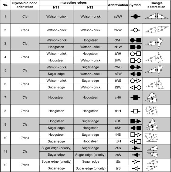Each geometric base pair family is defined by the interacting edges of the bases and the relative orientation of the glycosidic bonds (columns 2-4). Abbreviations and symbols for representing each base pair family in text and secondary structures are shown in columns 5 and 6. Column 7 shows an abstract representation of each family using triangles to represent the bases, where the hypotenuse represents the Hoogsteen edge. The shaded cells denote base pairs in the cis orientation.

Analysis using FR3D (7) of the 3D rRNA structures of the 70S ribosomes of E. coli and T. thermophilus and the 50S subunit of H. marismortui shows that ∼59% of all bases form canonical WC base pairs, including 7% that form a WC base pair and at least one non-WC base pair (Table 2). Of the remaining bases, approximately half (i.e. 20% of all bases) form one or more non-WC base pairs. Thus, a significant fraction (27%) of rRNA bases form non-WC base pairs. Furthermore, Table 2 shows that most of the remaining bases, none of which form base pairs, interact with other nucleotides through base-stacking or base-phosphate interactions.

Table 2.

Fraction of nucleotides in the 5S, 16S and 23S rRNA 3D structures of E. coli (PDB files: 2aw4 and 2avy) and T. thermophilus (PDB files: 2j01 and 1j5e) and the 5S and 23S rRNAs of H. marismortui (PDB file: 1s72) that form cWW and non-cWW base pairs, base-stacking and base–phosphate interactions

Bases forming base pairs
cWW base pairs and no non-cWW base pair	52%
cWW base pairs and at least one non-cWW base pairs	7%
At least one non-cWW base pairs and no cWW base pairs	20%
Bases forming other interactions (no base pairing)
Base-stacking and base–phosphate interaction	13%
Base–stacking only	3%
Base–phosphate only	1%
Bases forming no RNA–RNA interactions	4%
Total	100%

Base pair exemplars and online base pair catalog

To compare base pairs between and within geometric families, we have identified a single representative, called the exemplar, for each base combination (i.e. AA, AC, AG, …, UU) that makes a pair in a given geometric family as described in the ‘Materials and methods’ section. Thus, distinct exemplars were identified for cWW GC, cWW UA, tWH UA, etc. The base pair exemplars, organized by geometric family, are available online in the BGSU Basepair Catalog (http://rna.bgsu.edu/FR3D/basepairs/). Each base pair exemplar is the centroid of the collection of base pair instances of the same type and, as such, is an actual instance, not an average of some kind. While the instances of a particular base pair may show a wide range of variation, including twist and buckle, the exemplar is typically quite planar. For some base pairs, very few instances have been observed, and the automated procedure described above may not return the best instance of the base pair, so some base pairs are manually curated, either by selecting a particular instance or by substituting a modeled base pair where necessary. These cases are noted in the online Basepair Catalog.

Predicted base pairs observed in new structures

In the last compilation of base pairs, published in 2002 (1), we reported observations in new structures of several base pairs predicted in earlier compilations (16,17) and, in turn, predicted a number of additional base pairs, which had not yet been observed in 3D structures. A measure of the usefulness and generality of the geometric base pair classification is its ability to predict the occurrences and geometries of new base pairs. Thus, we carried out an exhaustive search of the current structure database to identify new base pair instances. This search produced examples for almost all remaining predicted base pairs. The new experimental instances were compared to the predicted base pairs and in most cases, the observed H-bonding patterns and approximate C1′–C1′ distances agree (Supplementary Table S5). We found one or more examples in 3D structures of several predicted base pairs: three cWS, tWS and cSS base pairs, two cHS and one tSS base pair. Furthermore, evidence that these base pairs occur in structured RNAs was found by analyzing alignments of 5S, 16S and 23S rRNA sequences at positions where the geometric family is conserved between the E. coli and T. thermophilus 3D structures, as will be described in more detail below in the section ‘Determination of base pair frequencies within geometric families from rRNA multiple sequence alignments’. The frequencies at which these newly observed base pairs occur, as inferred from sequence alignments, range from 0.1% to 2.2%, where the percentages refer to the fraction of base pairs in the geometric family to which each base pair belongs. The frequencies from sequence alignments of the newly observed base pairs are also given in Supplementary Table S5. At this point, there are only four predicted base pairs for which we have yet to find instances in structures: cWH AU and CU and tWS CU and UU. Sequence analysis indicates these are very rare, if they occur at all, with occurrence frequencies <0.3% in each case.

The IsoDiscrepancy Index (IDI)

In this section we review criteria for base pair isostericity and propose and evaluate a quantitative measure, the IDI.

Definition

While all base pairs belonging to the same family are geometrically similar, they are not necessarily identical or isosteric. To compare base pairs within and between families, we propose a quantitative measure of base pair isostericity, the IDI, which we define by analogy to the Geometric Discrepancy, a measure for the geometric similarity between two RNA motifs, that we previously developed to compare RNA motifs for geometric searches (7). The IDI quantifies those attributes of a base pair that affect its ability to substitute for another base pair without disturbing the geometry of the backbone. The IDI was designed so that two base pairs with sufficiently low IDI can be considered isosteric, as will be discussed in the section ‘Validation of the IDI’.

Note that while the position of the backbone is, of course, of great importance to RNA structure, it does not seem to be of primary importance when considering base pair substitutions. Indeed the same base pair (i.e. the same base combination and the same geometric family) in two different contexts can show a great deal of variation by RMSD of its backbone atoms, while the base pair itself looks the same in these different contexts. In particular, in some cases, a base may form a specific base pair by adopting the syn conformation, with concomitant dramatic changes in the sugar-phosphate backbone. Our notion of isostericity allows us to identify base combinations that could substitute for one another without disturbing the backbone, no matter what the context.

Therefore, we focus on the ribose glycosidic carbon atoms, C1′, and the base atoms to which they are bonded, N1 for pyrimidines and N9 for purines. The positions of the C1′ atoms are most constrained by being directly connected to the bases and the backbone, so we calculate C1′–C1′ distance between base paired nucleotides (18). In previous work, we qualitatively defined two base pairs as isosteric when three conditions are met: (i) the C1′–C1′ distances in the two pairs are nearly identical; (ii) the corresponding bases form hydrogen bonds between equivalent atoms and (iii) the bases in each pair are related by nearly identical rotation matrices. Now we translate these three criteria into quantitative terms as shown in Figure 1, using base pairs that differ sufficiently by one of these criteria to be non-isosteric. For criterion 1, we calculate the C1′–C1′ distance for each base pair and denote by Δc the difference in the C1′–C1′ distances. Next, for each base pair, we designate a ‘first’ and ‘second’ base. We translate the second base pair so that the N1/N9 atom of its first base coincides with the N1/N9 atom of the first base of the first base pair, then rotate the second base pair so that the glycosidic bonds of the first bases of each pair coincide, and finally rotate about the glycosidic bond to make the first bases co-planar, with the WC edges aligned. We say that the first bases are now in the same orientation. We next project the second bases onto the plane defined by the first bases. For criterion 2, we calculate the distance in the plane between the C1′ atoms of the second bases when the first bases have the same orientation, denoting this by t₁. For criterion 3, we distinguish two cases: Case 1 holds when the second bases can be brought into the same orientation by a rotation in the plane, for example when calculating the IDI for a cWW and a cWS base pair. The angle of rotation is denoted θ₁ and given in radians. Next we translate and rotate to bring the second bases of each base pair into the same orientation and calculate t₂ and θ₂ relative to the first bases. The distances t₁ and t₂ are, in general, different, so we calculate both and average them in the equations. For Case 1, we average the angles of rotation in the plane, θ₁ and θ₂, because they are not the same. We now calculate the IDI using this equation:

Figure 1.

Representation of the three contributions to the IDI illustrated using non-isosteric base pairs. To calculate the IDI for two base pairs, the bases designated ‘first base’ in each base pair are superposed (bases on the left in each panel) and then the following three quantities are evaluated, normalized and summed: (1) The difference, Δc, in the intra-base pair C1′–C1′ distances, illustrated for two non-isosteric cWW base pairs, AG and AU. (2) The inter-base pair C1′–C1′ distance, t₁, between the C1′ atoms of the second bases of the base pairs, illustrated for the near isosteric cWW AU and AC base pairs. We also calculate the corresponding distance t₂ after first superposing the second bases of the base pairs. (3) The angle, θ, about an axis perpendicular to the base pair plane, required to superpose the second bases, illustrated using non-isosteric cWW AU and cWS AU base pairs. For some pairs of base pairs, a 180° rotation (flip) about an axis in the base pair plane is required to superpose the second bases (case not shown).

Case 1 equation:

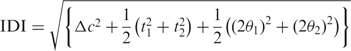It is not always possible to bring the second bases into the same orientation by rotating in the plane. For example, when calculating the IDI for a cWW and a tWW base pair, the second base of the second base pair must be flipped 180° (π radians) about an axis in the plane to bring it into the same orientation as the second base of the first base pair. This is Case 2 and the IDI is calculated with this equation:

Note that the rotation angle in Case 1 is multiplied by the coefficient 2. We can interpret 2θ₁ as the arc length, in Ångstroms, that an atom 2 Å from the N1/N9 atom would move when the base is rotated through the angle θ₁. This gives an indication of the effect that rotation has on the sugar ring of the nucleotide, and thus on the backbone itself. Thus, the IDI has units of Ångstroms, and measures on a single scale the various ways in which one base pair may differ from another in its effect on the backbone. The angle coefficient in Case 2 is larger, reflecting the greater effect of accomplishing a 180° rotation (π radians) of a base about the glycosidic bond. Third, because we calculate the shift and rotation angle twice, the IDI is symmetric with respect to the order that the base pairs are specified. Thus, the IDI between AG cWW and AG tHS is the same as between AG tHS and AG cWW or between GA cWW and GA tSH, but is not the same as between AG cWW and GA tSH.

Validation of the IDI

A quantitative measure of isostericity must be sensitive to structural differences between base pairs that are germane to their ability to substitute for one another in 3D structures. We evaluated the IDI by checking how it handles four distinct cases. First, the IDI should be lowest between instances of the same base pair. The upper-left panel of Figure 2 shows a histogram of the IDI calculated between each distinct pair of base pair instances of the same kind from 3D structures (i.e. GC cWW with GC cWW, UA tWH with UA tWH, etc.). The base pairs were drawn from the crystal structures in the reduced-redundancy dataset having a resolution better than 3.0 Å. At most 200 instances of each base combination from each geometric family were used to prevent the cWW base pairs from dominating the histogram. When more than 200 instances were available, 200 were selected randomly. The distribution peaks at IDI = ∼0.6 and is narrowly distributed as it should be when comparing identical base pairs, regardless of geometric family.

Figure 2.

Histograms of IDIs between sets of identical (upper left), isosteric (upper right), near isosteric (lower left) and non-isosteric (lower right) base pair instances from the 3D structures in the reduced-redundancy dataset having better than 3.0 Å resolution. Upper left: IDIs calculated between identical base pairs (i.e. GC cWW with GC cWW, UA tWH with UA tWH, etc.). Upper right: IDIs between 200 GC cWW and 200 UA cWW pairs. Lower left: IDIs between 200 GC cWW and 200 GU cWW pairs. Lower right: IDIs between 200 GU cWW and 200 UG cWW pairs.

Second, a quantitative measure of isostericity should be comparably low between base pairs classified as isosteric by qualitative criteria. In the upper-right panel of Figure 2 we show the IDI calculated between combinations of 200 GC and 200 UA cWW base pairs from the same 3D structures as described above. As in the first panel, the vast majority (over 96%) of comparisons result in an IDI below 2.0 and the distribution peaks below 1.0 and is similar in shape. Third, the IDI should be larger for base pairs that are near isosteric and known to occasionally substitute for one another. The lower-left panel of Figure 2 shows the IDI between 200 GC cWW and 200 GU cWW base pairs. The peak of the histogram occurs to the right of 2.0 and the distribution is largely non-overlapping with the distributions for isosteric or identical base pairs in the upper panels of Figure 2. Finally, the IDI should be largest for base pairs which are geometrically dissimilar (non-isosteric). The lower-right panel of Figure 2 shows the IDI between 200 GU cWW pairs and 200 UG cWW pairs. This distribution peaks at IDI = ∼4.5 and is largely non-overlapping with the others in Figure 2. When base pairs from different geometric families are compared, even larger IDI values are obtained, ranging up to 20. Histograms were also made using base pairs extracted from structures with 2.0 Å or better resolution. We observed that the corresponding IDI distributions from the 2.0 Å and 3.0 Å data peak within ∼0.2 Å of each other. As expected, the 2.0 Å IDI distributions were narrower, with full width at half height ∼0.5 Å vs. ∼0.8 Å for the 3.0 Å data. Based on these and similar analyses for non-WC base pairs, we chose IDI threshold values ≤ 2.0 for isosteric base pairs and 2.0 < IDI ≤ 3.3 for near isosteric base pairs.

IsoDiscrepancy between pairs within the same geometric family

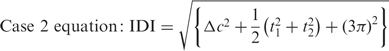
In Table 3, we show the matrix of IDI scores calculated between exemplars for each cWW base pair, color-coded to show which base pairs are isosteric (IDI ≤ 2.0), near isosteric (2.0 < IDI ≤ 3.3) or non-isosteric (IDI > 3.3). The base pairs are grouped together in each matrix by IDI score in blocks of isosteric or near isosteric base pairs. Corresponding matrices for each of the other 11 base pair families are provided in the Supplementary Table S6.

Table 3.

Matrix of IDI values for the cWW family

The IDI was calculated for each pair of cWW base pair exemplars, as indicated by the column and row labels. Cells in this and other tables are color-coded to reflect the IDI thresholds: (1) red: isosteric base pairs (IDI ≤ 2.0); (2) yellow: near isosteric base pairs (2.0 < IDI ≤ 3.3); (3) cyan: non-isosteric base pairs (moderate IDI: 3.3 < IDI ≤ 5.0); (4) blue: very different base pairs (large IDI: 5.0 < IDI). Base pairs are grouped to form isosteric and near isosteric blocks. The column labeled ‘LSW’ indicates the isosteric subgroups reported in (1). The column labeled ‘Count’ indicates the number of instances of the base pair observed in the reduced-redundancy set of structures.

The IDI provides a quantitative measure to group base pairs. The IDI is sensitive enough to distinguish isosteric from near isosteric base pairs in the same geometric family. The IDI clusters the standard WC base pairs (cWW AU, UA, GC and CG) and the near isosteric ‘wobble’ pairs (cWW GU and AC and cWW UG and CA) in distinct isosteric groups (IDI < 1.0 within each group). The canonical pairs are near isosteric to GU and AC and to UG and CA (IDI: 2.1–2.8) but the GU and AC are not isosteric to UG and CA (IDI: 4.5–5.0), consistent with the qualitative classification previously described (1).

In the section ‘Conservation of base pair families and isostericity in alignments of 3D structures’, we will evaluate how well the IDI and the proposed IDI cutoffs account for base pair substitutions observed in the 3D structures of E. coli and T. thermophilus 5S, 16S and 23S rRNAs.

Average IsoDiscrepancy within and between base pair families

We have calculated the average IDI between all pairs of base pair exemplars in each family and between families (Table 4). To prepare Table 4, the IDI was calculated between each base pair exemplar, i, in family X and each base pair exemplar, j, in family Y, taking the order of first and second bases which minimizes the average IDI between the families. Comparison of diagonal and off-diagonal elements of the matrix in Table 4 shows that the average IDI values within each family are smaller than those calculated between families, indicating that base pairs within each family are more similar to each other than to base pairs in other families. Furthermore, the IDI separates the geometric families into two distinct groups. The first group comprises cWW, tWH, cWS, cHH, tHS and cSS and the second comprises tWW, cWH, tWS, tHH, cHS and tSS. Base pair families belonging to the same group are related by rotations and translations of one base relative to the other, the second base within the plane of the first base. Consequently, with stereo-chemically identical nucleotides, the base pairs of the first group will lead to locally anti-parallel strands and those of the second group to locally parallel strands (2). In general, as previously noted (3), base pair families of one group are structurally more similar to each other than to families belonging to the other group.

Table 4.

Average IDIs within and between geometric families

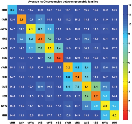The values shown in cells along the diagonal are the average IDIs within geometric base pairing families, while the values shown in off-diagonal cells are the average IDIs between base pairing families. For each pair of families, the minimum IDI was computed between each pair of exemplars, and averaged over all pairs. The families are arranged in the matrix to group similar families near one another, forming two main groups. Each cell is colored according to the scale on the right. All cells with IDIs above 12 are colored dark blue.

4 × 4 IDI SUBSTITUTION TABLES

The information provided in matrices of IDI values (Table 3 and Supplementary Data S6) can also be presented using a series of 4 × 4 matrices, examples of which are shown in Table 5, while the complete sets of matrices for each geometric family are in Supplementary Data S7. These matrices are used as follows: suppose that one observes an AU cWW base pair at a certain position in an RNA 3D structure and would like to know which base substitutions are isosteric or near isosteric to it. In this case, one consults the AU cWW 4 × 4 matrix (Table 5, left panel) to find the IDI values between all other cWW exemplars and the AU cWW exemplar. Similarly, one may consult the AG cWW 4 × 4 matrix (Table 5, middle panel) to find base pairs isosteric or near isosteric to AG cWW and so on. Comparison of the GU cWW 4 × 4 matrix (right panel of Table 5) with the one for AU cWW shows that while cWW AC, CA, GU and UG are all near isosteric to AU (yellow), UG and CA are not isosteric to GU cWW (cyan). These 4 × 4 matrices are relevant for evaluation and refinement of homologous RNA sequence alignments (see Discussion section).

Table 5.

Examples of 4 × 4 IDI substitution tables

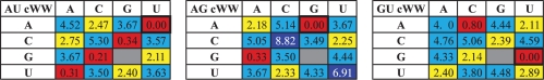IDI substitution tables for AU cWW (left), AG cWW (middle) and GU cWW (right) base pairs. These tables are specific to each base combination in each base pair family. Each table shows the IDI values between the base pair indicated in the upper left cell and all other base combinations in that family and is color-coded to show which base pair substitutions are isosteric (red), near isosteric (yellow) or non-isosteric (blue). Left panel: CG, GC and UA are isosteric to AU. Middle panel: GA is isosteric to AG. Right panel: AC is isosteric to GU. Tables for each combination and each base family are available in Supplementary Data S7.

Updated Isostericity Matrices (IM)

The previous section shows that it is not possible, without loss of information, to condense the IDI matrix for a geometric family into a single 4 × 4 matrix. This is because the IDI is not a transitive relation. Nonetheless the 4 × 4 IM, introduced in previous work to represent the subsets of mutually isosteric base pairs in each family, are also useful because they are so succinct (1). The matrix elements of IM are represented by ‘I_i.j,’ where i indexes the geometric family and j indexes the isosteric subset. We have revised and updated the IM using the IDI values calculated from base pair exemplars to cluster base pairs in each geometric family into isosteric subgroups. The updated IM for the tWH family is shown in Table 6 and the rest of the IM are in Supplementary Data S6. For most families, the IM changed minimally, with two or fewer base pairs re-assigned. More extensive changes were required only for the tWW, tHH and tWS families.

Table 6.

IM for the tWH family determined from IDI values (Supplementary Data S6)

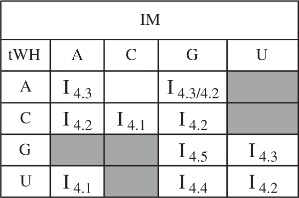The tWH base pairs UA and CC belong to isosteric group I_4.1, CA, CG, UU and AG belong to I_4.2, AA, AG and GU, I_4.3, while UG and GG each have their own isosteric groups, I_4.4 and I_4.5. Note that AG belongs to two groups, I_4.2 and I_4.3. The AU, CU, GA, GC and UC base combinations do not occur in this geometric family and their cells are shaded gray in the IM.

Base pair frequencies from 3D structures

To advance RNA structural bioinformatics, we require reliable estimates of base pair occurrence frequencies for geometric base pair families and for base combinations within each family. The most reliable source for these data are atomic-resolution 3D structures, available from the international repositories for biomolecular 3D structures, the Protein Data Bank (PDB) and the Nucleic Acid Database (NDB). For our analyses, we restricted ourselves to 3D structures determined by X-ray crystallography that have resolution better than 4.0 Å. Some poorly modeled structures were excluded, even though resolution better than 4.0 Å was reported. Because the PDB/NDB contains multiple entries for many RNA molecules that differ very little, if at all, in the structures of the RNA components, we selected a reduced-redundant dataset as described in the ‘Materials and methods’ section to avoid statistical bias that duplicate structures might introduce.

Structural analysis to obtain base pair frequencies

The reduced-redundancy 3D dataset was analyzed to compile base pair frequencies by base combination and base pair family. Each PDB file was analyzed using the structure analysis modules of FR3D to automatically identify, classify and list all WC and non-WC base pairs. The algorithm implemented in FR3D for base pair analysis has been described (7). The base pairs identified by FR3D for each RNA-containing PDB file are available at http://rna.bgsu.edu/FR3D/AnalyzedStructures/. The base pair analysis modules have been refined by carrying out multiple cycles of manual and automated analysis of the reduced-redundancy PDB data set. The lists obtained are in good agreement with lists produced manually by experts and are improvements over lists produced by other programs (19).

Relative frequencies of the geometric families from 3D data

Table 7 shows the occurrence frequencies by geometric base pair family obtained from 3D structures. We analyzed the entire reduced-redundancy dataset and, separately, representative 5S, 16S and 23S rRNA structures (PDB files: 1j5e, 2avy, 2j01, 2aw4 and 1s72). Table 7 shows that the rRNA structures are significantly enriched in non-WC base pairs compared to the entire dataset. For example, 7.3% of the base pairs in the rRNAs are tHS compared to 4.4% for the entire reduced-redundancy set. Overall, 67.5% of base pairs in the rRNA structures are cWW base pairs compared to 76.5% for the entire set. Base pair frequencies for rRNAs are reported separately because the rRNAs may be more representative of large, structured RNAs than the database as a whole.

Table 7.

Counts and frequencies of base pairs found in RNA 3D structures, by geometric base pair family

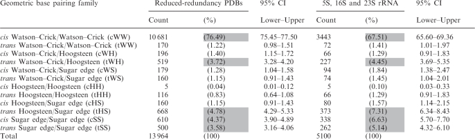For each base combination we report eight numbers; the first is the base pair count from the reduced-redundancy set of 3D structures, the second is the percentage this represents of the total and the third and fourth are simultaneous 95% CI for the frequencies reported as percentages. The second set of four numbers in each row reports the results obtained only using base pairs drawn from five representative rRNA structures [50S H. marismortui (PDB: 1s72), E. coli (PDB: 2aw4) and T. thermophilus (PDB: 2j01) and 30S E. coli (PDB: 2avy) and T. thermophilus (PDB: 1j5e)].

Among the non-WC base pairs, the tWH, tHS, cSS and tSS families occur most frequently (shaded cells in Table 7). The tWH and tHS base pairs frequently occur together in the same 3D motifs, for example, in the sarcin and loop E motifs (20,21). The cSS and tSS base pairs occur frequently in tertiary interactions, where they are also referred to as ‘A-minor motifs’ (22). These data confirm trends observed with smaller sets of data (19). The rarest base pairs are the cHH, as expected from the chemical groups involved.

We also report in Table 7 simultaneous 95% confidence intervals to give an indication of the reliability of the estimated occurrence frequencies. These are appropriate when estimating multinomial probabilities; each base pair can come from any of the 12 families, each with a different probability. The intervals are chosen so that, if new data were collected and these intervals re-calculated, 95% of the time, all 12 intervals would cover their respective true percentages. We used Quesenberry intervals, as described in (15), to calculate the 95% confidence intervals. Note that for small estimated frequencies, the confidence intervals are not symmetric around the estimated frequency.

Frequencies of base pairs within each geometric family from 3D data

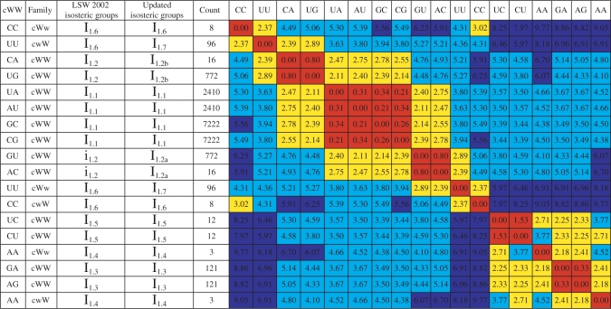
Table 8 shows base pair frequency data for the tWH base pair family. Comparable data tables for all other base pair families are provided in Supplementary Table S8. These tables provide base pair frequency estimates from 3D structures and from rRNA sequence alignments (to be described below) and 95% confidence intervals for these estimates as described in the Methods. Each cell of these 4 × 4 tables corresponds to a base combination (AA, AC, …, UU). Each cell contains data from four sources: (i) rRNA sequence alignments, (ii) E. coli rRNA 3D structures, (iii) T. thermophilus rRNA 3D structures and (iv) the entire reduced-redundancy 3D dataset. In Table 8, we treat each instance of a tWH base pair in a 3D structure as an independent observation. In rows 2, 3 and 4 of each cell we estimate the frequency with which pair XY occurs as a simple quotient of the number of XY base pairs observed divided by the total number of tWH pairs observed, and we use Quesenberry simultaneous 95% confidence intervals (15) to estimate multinomial frequencies. The calculations of occurrence frequencies from sequences (first row of each cell) will be explained in section ‘Determination of base pair frequencies within geometric families from rRNA multiple sequence alignments’.

Table 8.

Base pair counts and percent frequencies for the tWH base pair family, with simultaneous 95% CIs

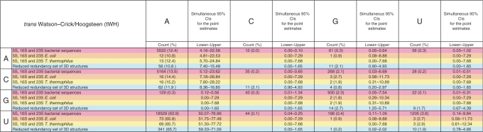Each cell contains data from four sources: (1) pink: 5S, 16S and 23S bacterial sequence alignments; (2) orange: 5S, 16S and 23S E. coli ribosome 3D structure (2avy and 2aw4); (3) yellow: 5S, 16S and 23S T. thermophilus ribosome structure [1j5e and 2j01(11,12)]; and (4) cyan: reduced-redundancy dataset of PDB files. For sequence alignments, the counts represent the number of instances of the respective base combination that occur in columns of the 5S, 16S and 23S rRNA sequence alignments (3,4) that correspond to tWH pairs in the conserved core of the 3D structural alignments. Corresponding tables for all 12 families appear in Supplementary Table S8.

Conservation of base pair families and isostericity in alignments of 3D structures

Now that we have atomic-resolution 3D structures of ribosomal RNAs from several organisms, we can compare them to study sequence variations at the level of 3D motifs and individual base pairs, as was done for Kink-turn and C-loop motifs in previous work (23). We ask whether the base substitutions that are observed for corresponding base pairs in homologous rRNAs tend to result in structurally similar (isosteric or near isosteric) base pairs. To make this comparison, we produced 3D structural alignments of the best available structures of the 5S and 23S rRNAs of E. coli, T. thermophilus and H. marismortui and the 16S rRNAs of E. coli and T. thermophilus The 3D structural alignments make it possible to identify base pairs that are likely to be conserved, at the level of the geometric family, in the respective aligned sequences.

rRNA 3D structural alignments

A 3D structural alignment shows which nucleotides in two or more 3D structures correspond to each other. It is based on a series of local superpositions between structural elements of two structures, nucleotide by nucleotide. 3D structural alignments were constructed for the rRNAs of E. coli, T. thermophilus and H. marismortui, using the PDB files 2awb and 2aw4 (E. coli), 2j01, 2j03 and 1vsa (T. thermophilus) and 1s72 (H. marismortui) for 5S and 23S rRNAs and PDB files 2aw7 and 2avy (E. coli) and 1j5e, 2j00, 2j02 and 2ow8 (T. thermophilus) for 16S rRNAs. The FR3D program suite was used to find and classify all base pairs in each crystal structure by geometric family (7). The lists of base pairs from each structure were imported and placed in columns of an Excel spreadsheet and manually aligned, as described in the Materials and methods section. The alignments for each molecule, 5S, 16S and 23S, are provided as separate worksheets in the Excel file included as Supplementary Table S9. A small portion of the structural alignment of 23S rRNA is shown in Figure 3a, along with annotated secondary structures (Figure 3b) and the E. coli 3D structure (Figure 3c) for comparison. Although the H. marismortui and E. coli sequences in this region differ at 13 out of 35 base positions (marked with shading in the H. marismortui alignment and secondary structure), the alignment and annotated structures show that the geometric types of the base pairs of the motif are conserved.

Figure 3.

Part of 3D structural alignment of E. coli and H. marismortui 23S rRNAs, illustrating structural conservation of a complex motif of Domain I that includes Helix 24. (a) The 3D structural alignment ofcorresponding base pairs from the E. coli (left) and H. marismortui (right) structures. (b) The annotated 2D structures for E. coli and H. marismortui using the base pair symbols. (c) Stereo view of the E. coli 3D structure, highlighting bases that differ between structures. The base pairs in the alignment and in the 2D and 3D structures are color-coded by geometric base pair family. Letters that correspond to bases which differ between organisms are marked in the secondary structure by a magenta circle and in the 3D structure with thicker lines.

Identifying the conserved core of bacterial rRNAs

The 3D alignments allow us to compare in detail the available rRNA structures, base pair by base pair, to determine the helices and 3D motifs that are conserved among the represented phylogenetic groups. The totality of conserved helices and 3D motifs between the E. coli and T. thermophilus rRNA structures constitutes the conserved bacterial core of each molecule. The base pairs of the conserved core were used to obtain base pair frequencies from rRNA sequence alignments, as described in section ‘Determination of base pair frequencies within geometric families from rRNA multiple sequence alignments’. The conserved core that we identified for bacterial 5S, 16S and 23S rRNAs from the structural alignments comprises, respectively 94%, 95% and 91%, of the total number of base pairs present in the respective rRNA structures. We also measured the IDI between the corresponding E. coli and T. thermophilus base pairs in the conserved core of each rRNA.

Base pair discrepancies between aligned positions in the rRNA 3D structural alignments

Within some otherwise conserved structural elements, we obtained high IDI scores for some isolated corresponding base pairs in the E. coli and T. thermophilus rRNA structures. Each of the ∼60 cases with IDI > 6.0 was examined manually and almost all fell into one of four categories. In the first case, which covers about two-third of the instances, the glycosidic-bond configuration (syn versus anti) is modeled differently for one of the corresponding nucleotides in the two structures. As a result, the structure with the syn base may lack the base pair entirely, because the bases are too far apart, or a different base pair may result. In the second case, the local sugar–phosphate backbone is modeled differently for the two structures, and again one structure may lack the base pair entirely or the E. coli and T. thermophilus base pairs belong to different base pair families. In the third case, the base pairs in the two structures belong to the same base pair family, but are not isosteric. In the fourth case, the base pairs in the two structures belong to different base pair families, although usually these are structurally related families.

An example of the first case is A353 in 16S rRNA, which was modeled syn in the E. coli structure but anti in T. thermophilus As a result, E. coli A353 cannot form the tertiary cSS base pair with G113 that is observed in the T. thermophilus structure. We called this and similar examples, whether they were modeled syn in the E. coli or in the T. thermophilus structures, to the attention of the crystallographers who solved these structures, for re-examination of the original or improved versions of their electron densities at these positions. In many cases they agreed that the configuration of the suspect nucleotide should be changed, usually from syn to anti. Thus, for E. coli A353, the correct configuration was identified as anti (Jamie Cate, Venki Ramakrishnan and Christine Dunham, private communications), indicating that the G113/A353 cSS base pair is conserved between the two structures. In all such cases, where the crystallographers agreed to change the glycosidic configuration and the change produced a base pair that agreed with the other structure in the context of an otherwise conserved motif, that base pairing position was added to the conserved core. Base pairs revised as a result of this comparative analysis were included in the alignment and are marked with the red text ‘Syn to Anti’ in column ‘O’ of the alignment to indicate revision of the cited PDB structure (Supplementary Table S9). However, the IDIs calculated using the original coordinates were retained in the alignment and are reported as such in column ‘N’.

In a very small number of instances, a syn base present in one structure results in a base pair belonging to a different family, but one which is structurally compatible in the structural context. In these cases reconsideration of the syn configuration was not justified. For example, G177 is syn in E. coli and forms a cHW pair with G145 while the corresponding C177 in T. thermophilus is anti and forms a cWW pair with G145. Nonetheless, both pairs are accommodated in helix 8 (h8) of 16S, because the C1′–C1′ distance in cWH GG (11.6 Å) is close to that of the WC pairs (∼10.5 Å) and the syn configuration of G177 guarantees the strands comprising h8 remain anti-parallel. However, the IDI in these cases is large.

An example of the second case, where there is a difference in modeling of the backbone, is the tertiary cWW base pair A64/U90, observed in the 23S rRNA of E. coli (2aw4) but not in T. thermophilus 23S (2j01). All other base pairs of this pseudoknot are present however, and the A64/U90 cWW base pair is present in the structure of T. thermophilus 23S rRNA (1vsa) solved by the Noller group (13). Therefore, we included this base pair in the conserved core. The third case, where two base pairs belong to the same family but the base pairs are not isosteric, occurs most often at the interface between a helix and 3D motif. An example occurs adjacent to the internal loop in h8 of 16S where non-isosteric cWW base pairs occur at equivalent positions, G148/A174 in E. coli and G148/C174 in T. thermophilus

The fourth case, where the corresponding base pairs belong to different families and are therefore non-isosteric, includes ∼20 instances. Most often these occur adjacent to 3D motifs of the rRNA. An example occurs in Helix 46 of 23S rRNA, where the base pair U1203/U1242 forms a ‘wobble’ cWW in E. coli, while at the equivalent positions G1203/A1242 forms a tSH base pair in T. thermophilus When the base pair type changes at two or more base pairing positions of corresponding motifs in the structures being compared, we define the positions as a ‘motif swap’ meaning substitution of one 3D motif by another that is functionally equivalent. Base pairs that belong to corresponding motifs that differ sufficiently to be classified as motif swaps were not included in the frequency analysis and will be discussed in future work. A number of discrepancies in the structural alignment were due to numbering errors between the E. coli and T. thermophilus due to insertions and deletions that were not handled in a consistent manner. These were resolved manually and made more conserved base pairs available for comparative sequence analysis.

IDI between aligned base pairs from the 3D structural alignments

The 3D structural alignment provides a way to directly assess the isostericity concept and its measurement using the IDI index. To make this evaluation, we first considered all the aligned base pairs in the 3D alignments that belong to the same geometric base pair family. Table 9 provides frequencies for the possible cases: (i) The same base combination occurs in both the E. coli and the T. thermophilus 3D structure; (ii) an isosteric substitution occurs, as determined using exemplars for the observed base pairs and the cutoffs as set above; (iii) a near isosteric substitution occurs and (iv) a non-isosteric substitution occurs. To calculate the IDIs we used exemplars for the aligned base pairs instead of the original coordinates. These data show that for 64% of the aligned cWW base pairs, the base combination is also conserved between the E. coli and T. thermophilus structures (e.g. UA cWW in both structures), while for the aligned non-cWW base pairs the base combination is conserved 85% of the time (e.g. UA tWH in both structures). The high conservation of the base combination for non-cWW base pairs is due to these base pairs usually being involved in more than one base pair interaction. Of the cWW base pairs where a substitution occurs, a large majority (24%) involves isosteric (e.g. UA cWW aligned to CG cWW) or near isosteric (10%) substitutions (e.g. UA cWW aligned to UG cWW) and very few involve non-isosteric (2%) substitutions (e.g. UA cWW aligned to AA cWW). For the non-cWW base pairs, when a substitution occurs, a majority (11%) involves isosteric (e.g. UA tWH aligned to CC tWH) or near isosteric (2%) substitutions (e.g. UA tWH aligned to UG tWH), while again only 2% are non-isosteric substitutions (e.g. UA tWH aligned to AA tWH).

Table 9.

Comparison of corresponding base pairs in the 3D structural alignment of E. coli and T. thermophilus 5S, 16S and 23S rRNAs

Comparison of corresponding base pairs from 3D alignment of E. coli and T. thermophilus rRNAs
	Identical BPs (%)	Isosteric BPs (%)	Near Isosteric BPs (%)	Non- Isosteric BPs (%)
cWW base pairs (1307 total)	64	24	10	2
non-cWW base pairs (720 total)	85	11	2	2
Total (2027 base pairs)	72	19	7	2

Row 1: cWW base pairs. Row 2: all other base pairs. Row 3: Combined cWW and non-cWW base pairs. Exemplars were used to calculate the IDIs for each aligned position in the 3D alignment to determine whether corresponding base pairs are isosteric, near isosteric or non-isosteric.

Second, we also calculated the IDI between all aligned base pairs, whether they are in the same geometric family or not, using the actual base pairs from the 3D structures. If isostericity is a valid hypothesis, the histogram of these IDIs should resemble the upper panels of Figure 2. The upper-left panel of Figure 4 shows the histogram of IDIs between all aligned base pairs. Clearly it has a more pronounced tail than the upper panels of Figure 2. We manually examined all aligned base pairs with IDI > 6.0. The instances with the largest IDI all have an Anti/Syn difference in one base of the two 3D structures. As discussed in section ‘Base pair discrepancies between aligned positions in the rRNA 3D structural alignments’ above, in most of these cases, the crystallographers agreed that the base in question should be changed from syn to anti, bringing the structures into agreement. Figure 4 (upper right) shows the IDIs between base pairs that are aligned and for which the family is conserved, excluding those in which an Anti/Syn change was confirmed by the crystallographers. The counts of IDI > 6.0 are significantly reduced, but there are still a significant number of counts in the IDI range 2.0–4.0. We split these cases into two categories and made separate histograms. In the lower-left panel, we tally instances in which both the geometric family and the base combination are conserved. The histogram closely resembles the upper-left panel of Figure 2. In the lower-right panel, we show instances in which the geometric family is conserved but the base combination is not. Relatively few IDIs exceed the near isosteric cutoff of 3.3, suggesting that, indeed, non-isosteric substitutions (i.e. IDI > 3.3) are rare when the geometric family is conserved. All in all, this analysis provides strong support for the isostericity hypothesis, but also reminds us that restricted regions of RNA molecules, particularly at the ends of some helices where most of the cases with IDI > 3.3 occur, are not under as much selection pressure to maintain isosteric base pair substitutions.

Figure 4.

Histograms of IDIs between actual base pairs in the 3D–3D alignment of E. coli and T. thermophilus 5S, 16S and 23S rRNAs. The IDIs used in these histograms were calculated before the revision of the 3D structures to correct syn-anti errors. The upper-left panel shows the IDI between all aligned base pairs, whether in the same geometric family or not. The base pairs with IDI > 6.0 are discussed in section ‘Base pair discrepancies between aligned positions in the rRNA 3D structural alignments’. The upper-right panel shows the IDI between aligned base pairs that belong to the same geometric family, and the lower panels subdivide these into two cases, those in which with identical base combinations (lower left) and those with different base combinations (lower right). All IDI values above 6 are placed in the rightmost bin in each histogram.

Determination of base pair frequencies within geometric families from rRNA multiple sequence alignments

The base pair frequency data from the 3D structure database, while very informative, are still too limited to estimate the frequencies of less common base pairs. Therefore, we turned to the extensive sequence databases that have been compiled for the 5S, 16S and 23S rRNAs to leverage the information contained in the 3D structures to obtain additional instances of base pairs from sequences. To do so accurately, we restricted our analysis to base pairs in the 3D structures of 5S, 16S and 23S rRNA that belong to structurally conserved motifs. This choice is based on the hypothesis that the base pair geometries of motifs that are conserved in the 3D rRNA structures of the distantly related bacteria E. coli and T. thermophilus will also be conserved in other bacterial rRNAs, which we know only from sequence data (24). The structural analysis described in section ‘IDI between aligned base pairs from the 3D structural alignments’ and summarized in Table 9 supports this hypothesis.

Therefore, we may also reasonably infer that the base pairs in the conserved core in the 3D alignments are also present in homologous molecules and are likely to form base pairs belonging to the same geometric base pair families. To obtain frequencies for each base pair family, we tabulated pairs of letters occurring in the columns corresponding to each base pair of that type. In this way, each instance of a base pair in the conserved bacterial core gives more observations of base pair combinations in that geometric family, so we can leverage the information from relatively few RNA 3D structures to gather information from a much larger dataset of RNA sequences. The base pair frequencies from sequence alignments and from 3D structures are compared in Table 8 for the tWH family. Supplementary Table S8 provides data for all the other base pair families. The Materials and methods section should be consulted on how we removed redundant sequences from the multiple sequence alignments used to obtain base pair frequencies; how base pairs in the 3D structure were selected for analysis and how we estimated confidence intervals for the base pair occurrence frequencies we obtained from the sequences and the 3D structures.

The reliability of the base pair frequencies determined from the sequence alignments depends critically on the quality of the sequence alignments. Misleading results can be obtained if a sequence does not in fact contain the base pair type inferred from the 3D structures or if the sequence is not aligned correctly to the structure, so the wrong base or a gap (‘-’) is placed in one of the columns. We can estimate the extent to which the data are affected by such errors by examining the frequencies of base combinations in the sequences which cannot form an allowed base pair in the geometric base pair family that occurs at the corresponding site of the 3D structure. For example, the base combination GG is not allowed at cWW base pairing positions, while CG, GA, GC, GU, UC and UU cannot occur at tHS sites. For the base pairs of the conserved core, the frequencies of non-allowed base combinations was <0.6% for all base combinations in all base pair families, with the exception of cWH AA (2.4%). In addition, very few gaps (<0.7%) occurred in the alignments at the positions included in the frequency analysis.

Base pair frequencies from rRNA

The sequences provide far more data than the 3D structures and so potentially provide more reliable estimates and narrower confidence intervals of base pair frequencies. These data, however, need some care in their interpretation. First, there are different numbers of sequences in the different multiple sequence alignment, 101 sequences for 5S rRNA, 717 sequences for 16S rRNA and 136 sequences for 23S rRNA. Second, the columns in the alignment corresponding to each base pair family in the conserved core may have gaps or letters other than A, C, G, U and these are counted as missing data for the purposes of this table.

We explain how we calculated the base pair frequencies from the sequence alignments using the tWH base pair family as an example: For each of the 95 instances of tWH base pairs in the conserved core of the 5S, 16S and 23S rRNA 3D alignments, we calculated the frequency (as a percentage) of each base combination in the corresponding two columns of the multiple sequence alignment. For each location in the 3D alignment, these frequencies add to 100%. Then we averaged the 95 sets of frequencies, thus giving equal weight to each location of a tWH base pair in the 3D structures, rather than weighting the data by the number of sequences available at each location. Even though we have dramatically reduced the redundancy within the aligned sequences, statistical dependence exists between the base combinations in the alignment corresponding to each particular instance of a tWH base pair in the conserved core. The simultaneous 95% confidence intervals derived from sequences (Table 8, row 1) are somewhat narrower than the confidence intervals calculated from the E. coli rRNA structures (Table 8, row 2) or the T. thermophilus rRNA structures (Table 8, row 3), but not as narrow as those obtained from the reduced-redundancy set of structures (Table 8, row 4). This indicates that using data from the multiple sequence alignment raises the effective number of observations above the total number of base pairs of a particular family in the rRNA 3D structures (i.e. 105 tWH base pairs in T. thermophilus 5S, 16S and 23S rRNA), but not as high as the total number of instances of that family in the reduced-redundancy 3D database (i.e. 519 tWH instances), or anywhere near the observed number of base combinations from the multiple sequence alignments (i.e. 8139 for tWH).

We provide a graphical summary of the base pair occurrence frequencies within each family, obtained from rRNA sequences, in Figure 5. The cWW, tWW, cHH and tHH families have symmetric base pairs; for example, each instance of GC cWW is also an instance of CG cWW. For this reason, we only display the data on upper right half of the matrices for these families. It is interesting to note that across the ribosomal structures, none of the base combinations in these four families show a 5′ to 3′ asymmetry due to order in the nucleotide sequence. For example, ∼50% of the GC cWW base pairs have G occurring earlier in the nucleotide sequence than C, and 50% have C first in the nucleotide sequence.

Figure 5.

A graphical summary of the base pair occurrence frequencies within each base pair family, obtained from rRNA sequence data (data from Supplementary Table S8). For cWW, tHH, tWH, tHS, tWS and tSS, one base combination accounts for >50% of instances. The gray boxes in each matrix indicate base combinations that do not form that type of base pair. For example, there is no GG cWW base pair.

DISCUSSION

We have defined the IDI to quantify base pair isostericity and to evaluate the usefulness of the isostericity concept for understanding non-WC base pairs and RNA 3D motifs and their evolution. The Leontis–Westhof base pair classification groups all base pairs into 12 basic geometric families, according to the interacting edges, WC, Hoogsteen, or Sugar, and the relative orientations of the glycosidic bonds. Base pairs within the same family consistently have smaller IDIs than base pairs belonging to different families. Furthermore, the IDI identifies which base pairs in the same family are isosteric and which are near isosteric or non-isosteric.

We have chosen the most representative instance (exemplar) for each base combination and base pair family and have presented them in the BGSU Basepair Catalog available online (http://rna.bgsu.edu/FR3D/basepairs/). Using the IDI values determined from base pair exemplars, we have updated the IM for each base pair family. We note that a single 4 × 4 IM cannot accurately represent all isosteric or near isosteric relationships, because the IDI is not a transitive measure. Thus, while base pair A can be isosteric to both base pairs B and C, B and C are not necessarily isosteric to each other. Clearly the full n × n matrices of IDI values for each family, where n is the number of base pairs in a given base pair family, are most useful for RNA structural bioinformatics applications (Supplementary Data S6).

Using the IDI, we found that almost all base pair substitutions in the 3D structures of the rRNAs of the distantly related bacteria, E. coli and T. thermophilus, are isosteric or nearly isosteric. This result strongly supports the hypothesis that base pair isostericity is fundamental for understanding the rules of sequence transformation during RNA evolution. Isostericity indicates which base pairs can potentially substitute for each other when a motif is conserved. However, in a given structural and functional context, isostericity considerations alone cannot predict which base pairs substitute for each other because additional constraints may be at work.

Along these lines, this work shows how isostericity can be fruitfully applied to produce and refine high quality RNA sequence alignments based on one or more 3D structures. The IM can be used to evaluate the quality of sequence alignments by comparing the base pairs implied by the alignment with the base pairs observed at the homologous positions of the available 3D structures. For each putative base pair in the alignment, the letters in the corresponding columns can be extracted in the form of 4 × 4 contingency or covariation matrices and compared to the 4 × 4 IDI substitution matrices that correspond to the base pairs observed in the 3D structures (Table 5 and Supplementary Data S7). Alignments can be adjusted iteratively by manual or automated procedures to minimize IDI values at aligned positions in conserved motifs.

We have also used the available 3D and sequence data to obtain robust base pair frequencies for each possible base combination in each of the 12 base pair families. For several of the non-WC base pair families, an important result is that only one or two base combinations account for most of the occurrences of that base pair family: Thus, in the cWH family, UA and GG account for > 70% of base pairs; in tWH, UA > 65%; in tWS, AG and GU > 50%; in tHH, AA > 70%; in cHS AA and UG > 60%; in tHS, AG > 70%; in cSS, CA and AC > 50%; and in tSS, AG > 60%. In the tWW family, AA, AU and GC account for most cases while in the cWS family, base pairs in which A or C pair with the WC edge account for most base pairs. Moreover, in most families, certain base combinations are exceedingly rare. In fact, we have yet to find examples of cWH AU or CU, and these pairs may not exist to any appreciable extent. Likewise all the YY combinations in cSS are very rare, and UU has not been observed.

The frequency and IDI data are most powerful when used together. For example, all 16 base combinations in the cSS base pair family form base pairs that are isosteric to each other. However, certain base combinations occur very frequently, while others are very rare, if they occur at all, as noted above. In such cases, scoring schemes for structural bioinformatics applications and 3D modeling procedures should benefit by taking both base pair frequencies and IDI values into account.

It is interesting to observe that not all base pairs which have low IDI occur with the same or comparable frequencies at equivalent positions in structural sequence alignments. This is probably due to a combination of additional factors besides geometry. First, some base pairs are energetically more stable than others, due to the types or number of hydrogen bonds they form, together with differences in their stacking energies when forming specific 3D motifs. For example, 22 base pairs in the classification comprise one strong H-bond and one weak H-bond involving a polarized C–H bond. In all cases, the frequencies of these base pairs are significantly smaller than those of isosteric base pairs that have two strong H-bonds.

Second, other constraints may operate, as when the base pair contacts other bases or makes base–protein or base–phosphate interactions. These additional constraints may disfavor certain isosteric substitutions. For example, the cHS AA pair is never observed to replace cHS UG in sarcin motifs even though they are isosteric base pairs. The G in sarcin motifs always H-bonds with its WC edge to a phosphate oxygen in an interaction that an A cannot make. Furthermore, the U in the sarcin motif makes a tWH pair with an A on the other strand. Thus, it is worth reiterating, that the IDI only indicates which base combinations can substitute for each other in the absence of additional constraints, but cannot by itself predict which base combinations will be more common than others.

This work shows that base pair frequencies in structured RNAs are very context dependent. This is reflected in the 3D structural alignment of the distantly related E. coli and T. thermophilus rRNAs, where we observe that for the majority of aligned base pairing positions, when the base pair family is the same in the two structures, the base combination is also the same. This trend is also reflected in the bacterial rRNA sequence alignments. A preliminary analysis shows that for most cases of cWW bases for which the base combination is conserved in homologous sequences, one or both bases participate in additional base-specific interactions, such as additional base pairs, base–phosphate, or base–amino-acid interactions. Base stacking interactions probably play decisive roles in other cases. We have therefore reported base pair frequencies from several sources: A reduced-redundancy dataset of 3D structures from NDB, the E. coli and T. thermophilus rRNA 3D structures, and the rRNA sequence alignments. All these data agree, in large part, within the calculated 95% confidence limits, but these limits are in most cases fairly wide, for reasons explained above. We propose, therefore, that for other structured RNAs, the frequencies from the rRNA sequence alignments may be the most pertinent.

CONCLUSIONS

The new RNA structures that are being added to the 3D structure databases present new opportunities to improve our understanding of the relationships between RNA 3D structures, RNA sequence variations in homologous RNA molecules, and RNA molecular evolution. The geometric classification of RNA base pairs and the isostericity concept provide a framework for using 3D information to address RNA bioinformatic challenges. A goal of the RNA Ontology Consortium (ROC) is to create data pipelines to facilitate this process (25). The isostericity relations and the detailed information from the IDI will be useful in developing new statistical procedures to identify RNA sequences in genomes and to more accurately align homologous RNA sequences using all base pair information, including that pertaining to non-WC pairs. These data are also pertinent for designing and interpreting mutational studies to determine whether a certain RNA motif is present in an RNA molecule for which the 3D structure is not known. Isostericity will also enable us to evaluate the quality of multiple sequence alignments by comparison of the implied base pairs to those observed in relevant 3D structures. Therefore, the frequency data presented in this article will be periodically updated on the ROC website (http://roc.bgsu.edu/) as new structures and improved alignments become available. The procedures developed here to create and analyze 3D structural alignments can be applied to other families of functional RNAs that occur in diverse organisms, such as self-splicing introns, RNase P, riboswitches and other structured regulatory RNA motifs.

SUPPLEMENTARY DATA

Supplementary Data are available at NAR Online.

FUNDING

This work was supported by grants to NBL from the National Institutes of Health (2 R15GM055898-04), from the National Science Foundation (Research Coordination Network Grant No. 0443508), and from Bowling Green State University (Research Capacity Expansion Program, funded by the Ohio Board of Regents Research Incentive Fund). Funding for open access charge: National Science Foundation (Research Coordination Network Grant No. 0443508).

Conflict of interest statement. None declared.

REFERENCES

- 1.Leontis NB, Stombaugh J, Westhof E. The non-Watson-Crick base pairs and their associated isostericity matrices. Nucleic Acids Res. 2002;30:3497–3531. doi: 10.1093/nar/gkf481. [DOI] [PMC free article] [PubMed] [Google Scholar]
- 2.Leontis NB, Westhof E. Geometric nomenclature and classification of RNA base pairs. RNA. 2001;7:499–512. doi: 10.1017/s1355838201002515. [DOI] [PMC free article] [PubMed] [Google Scholar]
- 3.Griffiths-Jones S, Bateman A, Marshall M, Khanna A, Eddy SR. Rfam: an RNA family database. Nucleic Acids Res. 2003;31:439–441. doi: 10.1093/nar/gkg006. [DOI] [PMC free article] [PubMed] [Google Scholar]
- 4.Wuyts J, Perriere G, Van De Peer Y. The European ribosomal RNA database. Nucleic Acids Res. 2004;32:D101–D103. doi: 10.1093/nar/gkh065. [DOI] [PMC free article] [PubMed] [Google Scholar]
- 5.Deshpande N, Addess KJ, Bluhm WF, Merino-Ott JC, Townsend-Merino W, Zhang Q, Knezevich C, Xie L, Chen L, Feng Z, et al. The RCSB Protein Data Bank: a redesigned query system and relational database based on the mmCIF schema. Nucleic Acids Res. 2005;33:D233–D237. doi: 10.1093/nar/gki057. [DOI] [PMC free article] [PubMed] [Google Scholar]
- 6.Dutta S, Berman HM. Large macromolecular complexes in the Protein Data Bank: a status report. Structure. 2005;13:381–388. doi: 10.1016/j.str.2005.01.008. [DOI] [PubMed] [Google Scholar]
- 7.Sarver M, Zirbel CL, Stombaugh J, Mokdad A, Leontis NB. FR3D: finding local and composite recurrent structural motifs in RNA 3D structures. J. Math. Biol. 2008;56:215–252. doi: 10.1007/s00285-007-0110-x. [DOI] [PMC free article] [PubMed] [Google Scholar]
- 8.Sethi A, O'Donoghue P, Luthey-Schulten Z. Evolutionary profiles from the QR factorization of multiple sequence alignments. Proc. Natl Acad. Sci. USA. 2005;102:4045–4050. doi: 10.1073/pnas.0409715102. [DOI] [PMC free article] [PubMed] [Google Scholar]
- 9.Gendron P, Lemieux S, Major F. Quantitative analysis of nucleic acid three-dimensional structures. J. Mol. Biol. 2001;308:919–936. doi: 10.1006/jmbi.2001.4626. [DOI] [PubMed] [Google Scholar]
- 10.Schuwirth BS, Borovinskaya MA, Hau CW, Zhang W, Vila-Sanjurjo A, Holton JM, Cate JH. Structures of the bacterial ribosome at 3.5 A resolution. Science. 2005;310:827–834. doi: 10.1126/science.1117230. [DOI] [PubMed] [Google Scholar]
- 11.Wimberly BT, Brodersen DE, Clemons WM, Jr., Morgan-Warren RJ, Carter AP, Vonrhein C, Hartsch T, Ramakrishnan V. Structure of the 30S ribosomal subunit. Nature. 2000;407:327–339. doi: 10.1038/35030006. [DOI] [PubMed] [Google Scholar]
- 12.Selmer M, Dunham CM, Murphy FVt, Weixlbaumer A, Petry S, Kelley AC, Weir JR, Ramakrishnan V. Structure of the 70S ribosome complexed with mRNA and tRNA. Science. 2006;313:1935–1942. doi: 10.1126/science.1131127. [DOI] [PubMed] [Google Scholar]
- 13.Korostelev A, Trakhanov S, Laurberg M, Noller HF. Crystal structure of a 70S ribosome-tRNA complex reveals functional interactions and rearrangements. Cell. 2006;126:1065–1077. doi: 10.1016/j.cell.2006.08.032. [DOI] [PubMed] [Google Scholar]
- 14.Ban N, Nissen P, Hansen J, Moore PB, Steitz TA. The complete atomic structure of the large ribosomal subunit at 2.4 A resolution. Science. 2000;289:905–920. doi: 10.1126/science.289.5481.905. [DOI] [PubMed] [Google Scholar]
- 15.Genz A, Kwong K. Numerical evaluation of singular multivariate normal distributions. J. Stat. Comput. Simulation. 2000;68:1–21. [Google Scholar]
- 16.Leontis NB, Westhof E. Conserved geometrical base pairing patterns in RNA. Quart. Rev. Biophys. 1998;31:399–455. doi: 10.1017/s0033583599003479. [DOI] [PubMed] [Google Scholar]
- 17.Leontis NB, Westhof E. A common motif organizes the structure of multi-helix loops in 16 S and 23 S ribosomal RNAs. J. Mol. Biol. 1998;283:571–583. doi: 10.1006/jmbi.1998.2106. [DOI] [PubMed] [Google Scholar]
- 18.Nasalean L, Stombaugh J, Zirbel CL, Leontis NB. In: Non-Protein Coding RNAs. Walter NG, Woodson SA, Batey RT, editors. Berlin Heidelberg: Springer; 2009. pp. 1–26. [Google Scholar]
- 19.Yang H, Jossinet F, Leontis N, Chen L, Westbrook J, Berman H, Westhof E. Tools for the automatic identification and classification of RNA base pairs. Nucleic Acids Res. 2003;31:3450–3460. doi: 10.1093/nar/gkg529. [DOI] [PMC free article] [PubMed] [Google Scholar]
- 20.Leontis NB, Stombaugh J, Westhof E. Motif prediction in ribosomal RNAs Lessons and prospects for automated motif prediction in homologous RNA molecules. Biochimie. 2002;84:961–973. doi: 10.1016/s0300-9084(02)01463-3. [DOI] [PubMed] [Google Scholar]
- 21.Leontis NB, Westhof E. Analysis of RNA motifs. Curr. Opin. Struct. Biol. 2003;13:300–308. doi: 10.1016/s0959-440x(03)00076-9. [DOI] [PubMed] [Google Scholar]
- 22.Nissen P, Ippolito JA, Ban N, Moore PB, Steitz TA. RNA tertiary interactions in the large ribosomal subunit: the A-minor motif. Proc. Natl Acad. Sci. USA. 2001;98:4899–4903. doi: 10.1073/pnas.081082398. [DOI] [PMC free article] [PubMed] [Google Scholar]
- 23.Lescoute A, Leontis NB, Massire C, Westhof E. Recurrent structural RNA motifs, Isostericity Matrices and sequence alignments. Nucleic Acids Res. 2005;33:2395–2409. doi: 10.1093/nar/gki535. [DOI] [PMC free article] [PubMed] [Google Scholar]
- 24.Sheridan PP, Freeman KH, Brenchley JE. Estimated minimal divergence times of the major bacterial and archaeal phyla. Geomicrobiol. J. 2003;20:1–14. [Google Scholar]
- 25.Leontis NB, Altman RB, Berman HM, Brenner SE, Brown JW, Engelke DR, Harvey SC, Holbrook SR, Jossinet F, Lewis SE, et al. The RNA Ontology Consortium: an open invitation to the RNA community. RNA. 2006;12:533–541. doi: 10.1261/rna.2343206. [DOI] [PMC free article] [PubMed] [Google Scholar]
Associated Data
This section collects any data citations, data availability statements, or supplementary materials included in this article.