Regularized F-Measure Maximization for Feature Selection and Classification

Abstract

Receiver Operating Characteristic (ROC) analysis is a common tool for assessing the performance of various classifications. It gained much popularity in medical and other fields including biological markers and, diagnostic test. This is particularly due to the fact that in real-world problems misclassification costs are not known, and thus, ROC curve and related utility functions such as F-measure can be more meaningful performance measures. F-measure combines recall and precision into a global measure. In this paper, we propose a novel method through regularized F-measure maximization. The proposed method assigns different costs to positive and negative samples and does simultaneous feature selection and prediction with L₁ penalty. This method is useful especially when data set is highly unbalanced, or the labels for negative (positive) samples are missing. Our experiments with the benchmark, methylation, and high dimensional microarray data show that the performance of proposed algorithm is better or equivalent compared with the other popular classifiers in limited experiments.

1. Introduction

Receiver Operating Characteristic (ROC) analysis has received increasing attention in the recent statistics and machine learning literatures (Pepe [1, 2]; Pepe and Janes [3]; Provost and Fawcett [4]; Lasko et al. [5]; Kun et al. [6]). ROC analysis originates in signal detection theory and is widely used in medical statistics for visualization and comparison of performance of binary classifiers. Traditionally, evaluation of a classifier is done by minimizing an estimation of a generalization error or some other related measures (Vapnik [7]). However the accuracy (the rate of correct classification) of a model does not always work. In fact when the data are highly unbalanced, accuracy may be misleading, since the all-positive or all-negative classifiers may achieve very good classification rate. In real life applications, the situations for which the data sets are unbalanced arise frequently. Utility functions such as F-measure or AUC provide a better way for classifier evaluation, since they can assign different error costs for positive and negative samples.

When the goal is to achieve the best performance under a ROC-based utility functions, it may be better to build classifiers through directly optimizing the utility functions. In fact, optimizing the log-likelihood function or the mean-square error does not necessarily imply good ROC curve performance. Hence, several algorithms have been recently developed for optimizing the area under ROC curve (AUC) function (Freund et al. [8]; Cortes and Mohri [9]; Rakotomamonjy [10]), and they have been proven to work well with different degrees of success. However, there are not many methods proposed for F-measure maximization. Most approaches to date that we know of maximize F-measure using SVMs and do so by varying parameters in standard SVM in an attempt to maximize F-measure as much as possible (Musicant et al. [11]). While this may result in a “best possible” F-measure for a standard SVM, there is no evidence that this technique should produce an F-measure comparable with one from the classifier designed to specifically optimize F-measure. Jansche [12] proposed an approximation algorithm for F-measure maximization in the logistic regression framework. His method, however, gives extremely large values for the estimated parameters and creates too many steep gradients. It, therefore, either converges very slow or fails to converge for large datasets.

Our aim in this paper is to propose a novel algorithm that directly optimizes an approximation of the regularized F-measure. The regularization term can be an L₂, L₁ or a combination of L₁ and L₂ penalty based on different prior assumptions (Tibshirani [13, 14]; Wang et al. [15]). Due to the nature of L₁ penalty, our algorithm provides simultaneous feature selection and classification with L₁ penalty. The proposed algorithm can be easily applied to high dimensional microarray data. One advantage with this method is that it is very efficient when data is highly unbalanced, since it assigns different costs to the positive and negative samples.

The paper is organized as follows. In Section 2 we introduce the related concept of ROC and F-measure. The algorithm and the brief proof of its generalization bounds are proposed in Section 3. The computational experiments and performance evaluation are given in Section 4. Finally the conclusions and remarks are discussed in Section 5.

2. ROC Curves and F-Measure

In binary classification, a classifier attempts to map the instances into two classes: positive (p) and negative (n). There are four possible outcomes with the given classifier: true positives (TP), false positives (FP), true negatives (TN), and false negatives (FN). Table 1 summarizes these outcomes with their associated terminology. The number of positive instances is N_p = TP + FN. Similarly N_n = TN + FP is the number of negative instances.

Table 1.

Classification outcomes.

		Predicted		Total
		1	−1
True	1	TP	FN	Np
	−1	FP	TN	Nn
		Mp	Mn

From these counts the following statistics are derived:

$$\begin{array}{l}\text{tpr}=\frac{\text{TP}}{\text{TP}+\text{FN}},\hspace{1em}\hspace{1em}\text{tnr}=\frac{\text{TN}}{\text{TN}+\text{FP}},\\ \text{fpr}=\frac{\text{FP}}{\text{FP}+\text{TN}},\hspace{1em}\hspace{1em}\text{fnr}=\frac{\text{FN}}{\text{TP}+\text{FN}}\mathrm{,}\end{array}$$ (1)

where true positive rate (also called recall or sensitivity) is denoted by tpr and true negative rate (specificity) by tnr. False positive rate and false negative rate are denoted by fpr and fnr, respectively. Note that tnr = 1 − fpr, and fnr = 1 − tpr. We also define the precision Pr = TP/(TP + FP). ROC curves plot the true positive rate versus false positive rate by varying the threshold which is usually the probability of the membership to a class, distance to a decision surface, or a score produced by a decision function. In the ROC space, the upper left corner represents a perfect classification, while a diagonal line represents random classification. A point in ROC curve that lies upper left of another point represents a better model.

F-measure combines the true positive rate (recall) and precision Pr into a single utility function which is defined as γ-weighted harmonic mean:

$$F_{\gamma }=\frac{1}{\gamma (1/\text{tpr})+(1-\gamma )(1/\text{Pr})}\mathrm{,}\hspace{1em}\text{where}\hspace{0.17em}0\le \gamma \le 1.$$ (2)

F_γ can be expressed with TP, FP, and FN as follows:

$$F_{\gamma }=\frac{\text{TP}}{\text{TP}+\gamma \text{FN}+(1-\gamma )\text{FP}}$$ (3)

or equivalently

$$F_{\gamma }=\frac{\text{TP}}{\gamma N_{\text{p}}+(1-\gamma )M_{\text{p}}}\mathrm{,}$$ (4)

where N_p is the number of positive samples, and M_p = TP + FP. Clearly 0 ≤ F_γ ≤ 1 and F_γ = 1 only when all the data are classified correctly. Maximizing F-measure is equivalent to maximizing the weighted sensitivity and specificity. Therefore, maximizing F_γ will indirectly lead to maximize the area under ROC curve (AUC).

To optimize F_γ, we have to define TP, FN, and FP mathematically. We first introduce an indicator function

$$I(y\in C)=\{\begin{array}{cc}1,& \text{if}\hspace{0.17em}\hspace{0.17em}y\in C,\\ 0,& \text{if}\hspace{0.17em}\hspace{0.17em}y\hspace{0.17em}\hspace{0.17em}\notin \hspace{0.17em}C,\end{array}$$ (5)

where C is a set. Let y = f(w, x) be a classifier with coefficients (weights) w and input variable x, and let $\widehat{y}$ be the predicted value. Given n samples, D = {(x₁, y₁),…, (x_n, y_n)}, where x_i is a multidimensional input vector with dimension m and class label y_i ∈ {−1, 1}; TP, FN, and FP are given, respectively:

$$\begin{array}{ll}\text{TP}& ={\displaystyle \sum }_{i=1}^{n}I({\widehat{y}}_i=1)I(y_i=1),\\ \text{FN}& ={\displaystyle \sum }_{i=1}^{n}I({\widehat{y}}_i=-1)I(y_i=1),\end{array}$$ (6)

$$\begin{array}{ll}\text{FP}& ={\displaystyle \sum }_{i=1}^{n}I({\widehat{y}}_i=1)I(y_i=-1)\mathrm{.}\end{array}$$ (7)

It is clear that F-measure is a utility function that applies for the whole data set.

3. The Algorithm

Usually given a classifier with known parameters w, F-measure can be calculated with the test data to evaluate the performance of the model. The aim of this paper is, however, to learn a classifier and estimate the corresponding parameters w with a given training data D and regularized F-measure maximization. Since F_γ ∈ [0, 1], we have −log F_γ ∈ [0, ∞). Statistically F_γ is a probability that measures the proportion of samples correctly classified. Based on these observations, we can maximize the log F_γ in the maximum log likelihood framework. Different assumptions for the prior distribution of w will lead to different penalty terms. Given the coefficient vector w with dimension m, we have L₂ = (1/2)∑_{j = 1}^m|w_j|² for the assumption of Gaussian distribution and L₁ = ∑_{j = 1}^m|w_j| with that of Laplacian prior. In general, L₁ penalty encourages sparse solutions, while the classifiers with L₂ are more robust. We make TP, FN, and FP depend on w explicitly and maximize the following penalized F-measure functions:

$$\begin{array}{ll}{E}_1(\mathbf{w})& =\log F_{\gamma }(\text{TP}(\mathbf{w}),\text{FN}(\mathbf{w}),\text{FP}(\mathbf{w}))-\lambda {\displaystyle \sum }_{j=1}^m\left|w_j\right|,\\ E_2(\mathbf{w})& =\log F_{\gamma }(\text{TP}(\mathbf{w}),\text{FN}(\mathbf{w}),\text{FP}(\mathbf{w}))-\frac{1}{2}\lambda {\displaystyle \sum }_{j=1}^m|w_j{|}^2\mathrm{.}\end{array}$$ (8)

We have

$$\begin{array}{ll}\widehat{\mathbf{w}}& =\arg \underset{\widehat{\mathbf{w}}}{\hspace{0.17em}\max }\left\{\log F_{\gamma }(\text{TP}(\mathbf{w}),\text{FN}(\mathbf{w}),\text{FP}(\mathbf{w}))-\lambda {\displaystyle \sum }_{j=1}^m\left|w_j\right|\right\}\mathrm{,}\\ \widehat{\mathbf{w}}& =\arg \hspace{0.17em}\underset{\widehat{\mathbf{w}}}{\max }\left\{\log F_{\gamma }(\text{TP}(\mathbf{w}),\text{FN}(\mathbf{w}),\text{FP}(\mathbf{w}))-\frac{1}{2}\lambda {\displaystyle \sum }_{j=1}^m|w_j{|}^2\right\}\mathrm{.}\end{array}$$ (9)

Note that TP(w), FN(w), and FP(w) are all integers, and the index function I in (7) is not differentiable. We first define an S-type function to approximate the index function I: Let z = w^Tx be a linear score function,

$$h(z)=\{\begin{array}{cc}0,\hfill & z\hspace{0.17em}<-1,\hfill \\ \frac{1}{2}{(1+z)}^2,\hfill & -1\le z\le 0,\hfill \\ \frac{1}{2}(2-{(1-z)}^2),\hfill & 0\hspace{0.17em}<\hspace{0.17em}z\le 1,\hfill \\ 1,\hfill & z\hspace{0.17em}>\hspace{0.17em}1.\hfill \end{array}$$ (10)

The decision role such that $\widehat{y}(\mathbf{w}\mathrm{,}\mathbf{x})=1$ if z = w^Tx > 0 can be represented as

$$I(\widehat{y}=1)=I(z>0)=I(h({\mathbf{w}}^T\mathbf{x})>0.5)\approx h({\mathbf{w}}^T\mathbf{x})\mathrm{.}$$ (11)

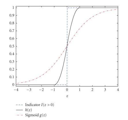
Figure 1 gives some insight about the h(z). Figure 1 shows that h(z) is a better approximation of I(z > 0) than the sigmoid function g(z) = 1/(1 + e^−z). The first derivative of h(z) is continuous and given in (12):

$$h^{\prime }(z)=\frac{dh(z)}{dz}=\{\begin{array}{cc}0,\hfill & z\hspace{0.17em}<-1,\hfill \\ 1\hspace{0.17em}+\hspace{0.17em}z,\hfill & -1\le z\le 0,\hfill \\ 1-z,\hfill & 0\hspace{0.17em}<\hspace{0.17em}z\le 1,\hfill \\ 0,\hfill & z\hspace{0.17em}>\hspace{0.17em}1.\hfill \end{array}$$ (12)

Based on (10) and (11), the approximated version of TP(w) and M_p(w) = TP(w) + FP(w) can be written as follows:

$$\begin{array}{ll}\text{TP}(\mathbf{w})& ={\displaystyle \sum }_{\begin{array}{c}i=1\\ y_i=1\end{array}}^{n}h({\mathbf{w}}^T{\mathbf{x}}_i),\\ M_{\text{p}}(\mathbf{w})& ={\displaystyle \sum }_{i=1}^{n}h({\mathbf{w}}^T{\mathbf{x}}_i)\mathrm{.}\end{array}$$ (13)

We can find the first-order derivatives of E₁ and E₂, respectively, as follows:

$$\begin{array}{ll}\frac{\partial E_1(\mathbf{w})}{\partial w_j}& =\frac{\partial F_{\gamma }(\mathbf{w})/\partial w_j}{F_{\gamma }(\mathbf{w})}-\lambda \hspace{0.17em}\hspace{0.17em}\text{sign}\hspace{0.17em}(w_j),\\ \frac{\partial E_2(\mathbf{w})}{\partial w_j}& =\frac{\partial F_{\gamma }(\mathbf{w})/\partial w_j}{F_{\gamma }(\mathbf{w})}-\lambda w_j\mathrm{,}\end{array}$$ (14)

where,

$$\begin{array}{c}\frac{\partial F_{\gamma }(\mathbf{w})}{\partial w_j}=B\frac{\partial \text{TP}(\mathbf{w})}{\partial w_j}-B^2\text{TP}(\mathbf{w})(1-\gamma )\frac{\partial M_{\text{p}}(\mathbf{w})}{\partial w_j}\mathrm{,}\\ B=\frac{1}{\gamma N_p+(1-\gamma )M_{\text{p}}(\mathbf{w})}\mathrm{,}\\ \frac{\partial \text{TP}(\mathbf{w})}{\partial w_j}={\displaystyle \sum }_{\begin{array}{c}i=1\\ y_i=1\end{array}}^n{h}^{\prime }({\mathbf{w}}^T\mathbf{x})x_{ij}\mathrm{,}\\ \frac{\partial M_{\text{p}}(\mathbf{w})}{\partial w_j}={\displaystyle \sum }_{i=1}^n{h}^{\prime }({\mathbf{w}}^T\mathbf{x})x_{ij}\mathrm{.}\end{array}$$ (15)

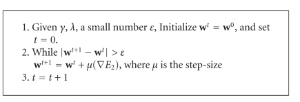
Knowing E₁ and E₂, and their derivatives ∇E₁ = [∂E₁/∂w_j] and ∇E₂ = [∂E₂/∂w_j], we can maximize the penalized function E₁ and E₂ with gradient descent-related algorithm such as Broyden-Fletcher-Goldfarb-Shanno- (BFGS-) related quasi-Newton method (Broyden [16]). The algorithm for E₂ maximization is straight forward as shown in Algorithm 1. The step-size μ in the algorithm can be found with line search.

Figure 1.

The plot for h(z), indicator function I(z > 0), and Sigmoid g(z) = 1/(1 + e^−z).

Algorithm 1.

L₂ regularized F-measure maximization.

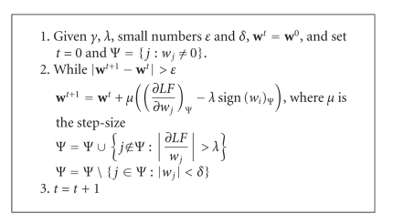
The regularized F-measure maximization with L₁ penalty (E₁) is of especial interest because it favors sparse solutions and can select features automatically. However, maximizing E₁ is a little bit complex since L₁ and E₁ are not differentiable at 0. For simplicity, let LF = log F_γ(w), we have E₁ = LF − λ∑_{j = 1}^m|w_j|. The Karush-Kuhn-Tucker (KKT) conditions for optimality are given as follows:

$$\begin{array}{cc}\hfill \left|\frac{\partial LF}{\partial w_j}\right|<\lambda & \Rightarrow w_j=0,\hfill \\ \hfill w_j\ne 0& \Rightarrow \left|\frac{\partial LF}{\partial w_j}\right|=\lambda \mathrm{.}\hfill \end{array}$$ (16)

The KKT conditions tell us that we have a set Ψ of nonzero coefficients which corresponds to the variables whose absolute value of first-order derivative is maximal and equal to λ, and that all variables with smaller derivatives have zero coefficients at the optimal penalized solution. Since L₁ is differentiable everywhere except at 0, we can design an algorithm to deal with the nonzero coefficients only. Algorithm 2 proposes an algorithm that can be applied to the subspace of nonzero coefficient set denoted by Ψ. The algorithm has a procedure to add or remove variables from Ψ, when the first-order derivative becomes large and when a coefficient hits 0, respectively.

Algorithm 2.

L₁ regularized F-measure maximization.

3.1. Computational Considerations

Both γ and λ are free parameters that need to be chosen. We will choose the best parameter for γ and λ with the area under ROC curve (AUC). Area under the ROC curve (AUC) is another scalar measure for classifier comparison. Its value is between (0, 1). Larger AUC values indicate better classifier performance across the full range of possible thresholds. For datasets with skewed class or cost distribution is unknown as in our applications, AUC is a better measure than prediction accuracy.

Given a binary classification problem with N_p positive class samples and N_n negative class samples, let f(x) be the score function to rank a sample x. AUC is the probability that a classifier will rank a randomly chosen positive instance higher than a randomly chosen negative instance. Mathematically

$$\text{AUC}=\frac{{\sum }_{i=1}^{N_{\text{p}}}{\sum }_{j=1}^{N_{\text{n}}}I(f({\mathbf{x}}_i)>f({\mathbf{y}}_j))}{N_{\text{p}}{N}_{\text{n}}}\mathrm{,}$$ (17)

where I(·) is an index function and I(·) = 1 if f(x_i) > f(y_j), otherwise I(·) = 0. AUC is also called Wilcoxon-Mann-Whitney statistic (Rakotomamonjy [10]).

Note that log F_γ(w) is generally a nonconcave function with respect to w; only local maximum is guaranteed. One way to deal with this difficulty is to employ the multiple-points initialization. Multiple random points are generated, and our proposed algorithms are used to find the maximum for each point. The result with the lowest test error is chosen as our best solution.

4. Computational Results

4.1. Benchmark Data

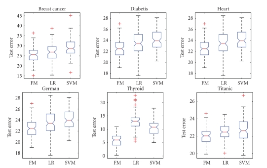
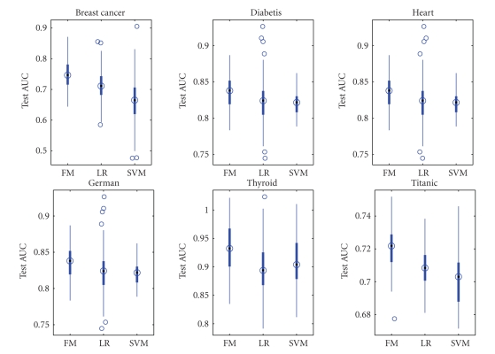
To evaluate the performance of the proposed method, experiments were performed on six benchmark datasets which can be downloaded from http://ida.first.fraunhofer.de/projects/bench/benchmarks.htm. These benchmark datasets have been widely used in model comparison studies in machine learning. They are all binary classification problems, and the datasets were randomly divided into train and test data 100 times to prevent bias and overfitting. The data are normalized with zero mean and standard deviation. The overview of the datasets is given in Table 2. The computational results with our algorithms, logistic regression, and linear support vector machines are given in Figures 2-3.

Table 2.

Overview of the datasets.

Datasets	No. of samples (train/test)	No. of variables	No. of experiments
Breast cancer	200/77	9	100
Diabetis	468/300	8	100
Heart	170/100	13	100
German	700/300	20	100
Thyroid	140/75	5	100
Titanic	150/2051	3	100

Figure 2.

Test Errors of L₂ F-Measure (FM), Logistic Regression (LR), and SVM.

Figure 3.

Test AUC of L₂ F-Measure (FM), Logistic Regression (LR), and SVM.

Figures 2-3 show that L₂ F-measure maximization performs better or equivalent compared with logistic regression and linear support vector machines (SVM) in limited experiments. In fact, the test errors for all datasets except for Thyroid are competitive with that of the nonlinear classification methods reported by Ratsch (http://ida.first.fraunhofer.de/projects/bench/benchmarks.htm). The inferior performance of L₂ F-measure with Thyroid data indicates the strong nonlinear factors in that data.

4.2. Real Methylation Data

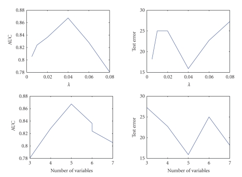
This methylation data are from 7 CpG regions and 87 lung cancer cell lines (Virmani et al. [17], Siegmund et al. [18]). 41 lines are from small cell lung cancer and 46 lines from nonsmall cell lung cancer. The proportion of positive values for the different regions ranges from 39% to 100% for the small cell lung cancer and from 65% to 98% for the nonsmall cell lung cancer. The data are available at http://www-rcf.usc.edu/kims/SupplementaryInfo.html. We utilize the twofold cross validation scheme to choose the best λ and test our algorithms. Other cross-validation schemes such as 10-fold cross validation will lead to similar results but are more computational intensive. We randomly split the data into two roughly equal-sized subsets and build the classifier with one subset and test it with the other. To avoid the bias arising from a particular partition, the procedure is repeated 100 times, each time splitting the data randomly into two folds and doing the cross validation. The average computational results with different γs and λ = 0.05 are given in Table 3. Table 3 shows the selected variables (1: selected; 0: not selected), sensitivity, specificity, test errors, and AUC values with different γ's. We can see clearly the sensitivity increases while the specificity decreases as γ increases. When γ = 0.9, every example is classified as positive examples. The best γ will be 0.4 according to AUC but it will be 0.2 based on test error. Therefore, again there is some inconsistence between two measures. Figure 4 gives some sight about how to choose λ and the number of features. Given γ = 0.4, the optimal λ = 0.04, and those 5 out of 7 CpG regions selected by L₁ F-measure maximization have been proved to be predictive of lung cancer subtype (Siegmund et al. [18]). The performance of the model is improved roughly 6% in AUC and 3% in test error with only 5 instead of 7 CpG regions.

Table 3.

Performance with different γ's and L₁ F-measure maximization.

γ	Variables selected (1/0)	Sensitivity	Specificity	Test error	AUC
0.1	1101111	0.476	0.957	27.3	0.801
0.2	1111111	0.714	0.957	15.9	0.820
0.3	0101111	0.810	0.740	22.7	0.849
0.4	1111001	0.826	0.762	20.4	0.861
0.5	1111101	0.857	0.609	27.3	0.832
0.6	1100101	0.762	0.739	25	0.832
0.7	1110110	0.904	0.348	38	0.847
0.8	1011100	100	0.217	40.9	0.826
0.9	1100011	100	0	52.3	0.754

Figure 4.

Performance with different λs and number of variables.

4.3. High Dimensional Microarray Data

The colon microarray data set (Alon et al. [19]) has 2000 features (genes) per sample and 62 samples which consisted 22 normal and 40 cancer tissues. The task is to distinguish tumor from normal tissues. The data set was first normalized for each gene to have zero mean and unit variance. The transformed data was then used for all the experiments. We employed a same twofold cross validation scheme to evaluate the model. This computational experiments are repeated 100 times. The AUC was calculated after each cross validation. The computational results for performance comparison are reported in Table 4.

Table 4.

Performance with different γ's and L₁ F-measure maximization (λ = 3).

γ	No. of variables	FN	FP	No. of misclassified	AUC
0.1	10	11	33	44	0.588
0.2	10	3	3	6	0.989
0.3	10	3	3	6	0.989
0.4	10	3	3	6	0.989
0.5	10	3	3	6	0.989
0.6	10	3	3	6	0.989
0.7	10	2	3	5	0.993
0.8	10	2	3	5	0.993
0.9	10	2	5	7	0.988
1	10	2	8	10	0.971

Table 4 gives us some insight that how the model performance changes with different γ's. Generally we can see that the false negative (FN) decreases and the false positive (FP) increases as γ increases. The only exception is when γ = 0.1, both FN and FP have the worst performance. The best performance is achieved when γ ∈ [0.7, 0.8] according to both AUC and the number of misclassified samples.

The 10 genes selected are given in Table 5. The selected genes allow the separation of cancer from normal samples in the gene expression map. Some genes were selected because their activities resulted in the difference in the tissue composition between normal and cancer tissue. Other genes were selected because they played a role in cancer formation or cell proliferation. It was not surprise that some genes implicated in other types of cancer such as breast and prostate cancers were identified in the context of colon cancer because these tissue types shared similarity. Our method is supported by the meaningful biological interpretation of selected genes. For instance, three muscle-related genes (H20709, T92451, and J02854) were selected from the colon cancer data, reflecting the fact that normal colon tissue had higher muscle content, whereas colon cancer tissue had lower muscle content (biased toward epithelial cells), and the selection of x12671 ribosomal protein agreed with an observation that ribosomal protein genes had lower expression in normal than in cancer colon tissue.

Table 5.

10 differentially expressed genes.

Gene ID	Description
h20709	myosin light chain alkali, smooth-muscle isoform (human)
t71025	84103 human (human)
m76378	human cysteine-rich protein (crp) gene, exons 5 and 6
m63391	human desmin gene, complete cds
z50753	h.sapiens mrna for gcap-ii/uroguanylin precursor
r87126	myosin heavy chain, nonmuscle (gallus gallus)
x12671	human gene for heterogeneous nuclear ribonucleoprotein (hnrnp) core protein a1
t92451	tropomyosin, fibroblast and epithelial muscle-type (human)
j02854	myosin regulatory light chain 2, smooth muscle isoform (human); contains element tar1 repetitive element
m36634	human vasoactive intestinal peptide (vip) mrna, complete cds

5. Conclusions and Remarks

We have presented a novel regularized F-measure maximization for feature selection and classification. This technique directly maximizes the tradeoff between specificity and sensitivity. Regularization with L₂ and L₁ allows the algorithm to converge quickly and to do simultaneous feature selection and classification. We found that it has better or equivalent performances when compared with the other popular classifiers in limited experiments.

The proposed method has the ability to incorporate nonstandard tradeoffs between sensitivity and specificity with different γ. It is well suited for dealing with unbalanced data or data with missing negative (positive) samples. For instance, in the problem of gene function prediction, the available information is only about positive samples. In other words, we know which genes have the function of interested, while it is generally unclear which genes do not have the function. Most standard classification methods will fail but our method can train the model with only positive labels by setting γ = 1.

One difficulty with the regularized F-measure maximization is the nonconcavity of the error function. We utilized the random multiple points initialization to find the optimal solutions. More efficient algorithms for nonconcave optimization will be considered to speed up the computations. The applications of the proposed method in gene function predictions and others will be explored in the future.

References

- 1.Pepe MS. The Statistical Evaluation of Medical Tests for Classification and Prediction. Oxford, UK: Oxford University Press; 2003. [Google Scholar]
- 2.Pepe MS. Evaluating technologies for classification and prediction in medicine. Statistics in Medicine. 2005;24(24):3687–3696. doi: 10.1002/sim.2431. [DOI] [PubMed] [Google Scholar]
- 3.Pepe MS, Janes H. Insights into latent class analysis of diagnostic test performance. Biostatistics. 2007;8(2):474–484. doi: 10.1093/biostatistics/kxl038. [DOI] [PubMed] [Google Scholar]
- 4.Provost F, Fawcett T. Robust classification for imprecise environments. Machine Learning. 2001;42(3):203–231. [Google Scholar]
- 5.Lasko TA, Bhagwat JG, Zou KH, Ohno-Machado L. The use of receiver operating characteristic curves in biomedical informatics. Journal of Biomedical Informatics. 2005;38(5):404–415. doi: 10.1016/j.jbi.2005.02.008. [DOI] [PubMed] [Google Scholar]
- 6.Kun D, Bourke C, Scott S, Vinodchandran NV. New algorithms for optimizing multi-class classifiers via ROC surfaces. In: Proceedings of the 3rd Workshop on ROC Analysis in Machine Learning (ROCML '06); June 2006; Pittsburgh, Pa, USA. pp. 17–24. [Google Scholar]
- 7.Vapnik V. The Nature of Statistical Learning Theory. New York, NY, USA: Springer; 1995. [Google Scholar]
- 8.Freund Y, Iyer R, Schapire RE, Singer Y. An efficient boosting algorithm for combining preferences. Journal of Machine Learning Research. 2004;4(6):933–969. [Google Scholar]
- 9.Cortes C, Mohri M. Advances in Neural Information Processing Systems 16. Cambridge, Mass, USA: MIT Press; 2003. AUC optimization vs. error rate minimization; pp. 313–320. [Google Scholar]
- 10.Rakotomamonjy A. Optimizing AUC with Support Vector Machine (SVM). In: Proceedings of European Conference on Artificial Intelligence Workshop on ROC Curve and AI; 2004; Valencia, Spain. [Google Scholar]
- 11.Musicant DR, Kumar V, Ozgur A. Optimizing F-measure with support vector machines. In: Proceedings of the 16th International Florida Artificial Intelligence Research Society Conference (FLAIRS '03); May 2003; St. Augustine, Fla, USA. pp. 356–360. [Google Scholar]
- 12.Jansche M. Maximum expected F-measure training of logistic regression models. In: Proceedings of the Conference on Human Language Technology and Empirical Methods in Natural Language Processing (HLT-EMNLP '05); October 2005; Vancouver, Canada. pp. 692–699. [Google Scholar]
- 13.Tibshirani R. Regression shrinkage and selection via the lasso. Journal of the Royal Statistical Society. Series B. 1996;58(1):267–288. [Google Scholar]
- 14.Tibshirani R. The lasso method for variable selection in the Cox model. Statistics in Medicine. 1997;16(4):385–395. doi: 10.1002/(sici)1097-0258(19970228)16:4<385::aid-sim380>3.0.co;2-3. [DOI] [PubMed] [Google Scholar]
- 15.Wang L, Zhu J, Zou H. The doubly regularized support vector machine. Statistica Sinica. 2006;16(2):589–615. [Google Scholar]
- 16.Broyden CG. Quasi-Newton methods and their application to function minimization. Mathematics of Computation. 1967;21(99):368–381. [Google Scholar]
- 17.Virmani AK, Tsou JA, Siegmund KD, et al. Hierarchical clustering of lung cancer cell lines using DNA methylation markers. Cancer Epidemiology Biomarkers & Prevention. 2002;11(3):291–297. [PubMed] [Google Scholar]
- 18.Siegmund KD, Laird PW, Laird-Offringa IA. A comparison of cluster analysis methods using DNA methylation data. Bioinformatics. 2004;20(12):1896–1904. doi: 10.1093/bioinformatics/bth176. [DOI] [PubMed] [Google Scholar]
- 19.Alon U, Barkai N, Notterman DA, et al. Broad patterns of gene expression revealed by clustering analysis of tumor and normal colon tissues probed by oligonucleotide arrays. Proceedings of the National Academy of Sciences of the United States of America. 1999;96(12):6745–6750. doi: 10.1073/pnas.96.12.6745. [DOI] [PMC free article] [PubMed] [Google Scholar]