

Abstract
The goal of measurements of the resisting force generated by a molecular bond as it is being forcibly separated under controlled conditions is to determine functional characteristics of the bond. Here, we establish the dependence of force history during unbinding on both those parameters chosen to characterize the bond itself and the controllable loading parameters. This is pursued for the practical range of behavior in which unbinding occurs diffusively rather than ballistically, building on the classic work of Kramers. For a bond represented by a one-dimensional energy landscape, modified by a second time-dependent energy profile representing applied loading, we present a mathematical analysis showing the dependence of the resistance of the bond-on-bond well shape, general time dependence of the imposed loading, and stiffness of the loading apparatus. The quality of the result is established through comparison with full numerical solutions of the underlying Smoluchowski equation.
Keywords: Kramers' theory, force spectroscopy, bond survival probability
Over the past decade, a number of reports of direct measurement of the mechanical strength of noncovalent bonds between adhering bioproteins have appeared. A major step forward was made by Evans and Ritchie (1) with the development and application of the biomembrane force probe. Other observations have been based on the atomic force microscope, optically trapped beads, and magnetically trapped beads. The experiments are brilliantly conceived but difficult to perform. The data provide an intriguing glimpse into the nanoscopic realm of material structure and its evolution. The data also provide a challenge, namely, to develop a quantitative characterization of bond features that can account for observed behavior.
The process of protein–protein debonding is described functionally as a transition from one stable configuration of the system to another, with passage through an unstable intermediate configuration in the process. In this development, we adopt the common point of view whereby the instantaneous state is identified by a single configuration variable x, akin to a reaction coordinate, and by a configurational free energy  (x,t) representing an energy landscape to which accessible configurations of the bond are confined. The present discussion is concerned with landscapes in one space dimension that may evolve over time. It is tacitly assumed that the energy landscape incorporates all energy changes which occur in bond separation and that the landscape for a given bond pair is indistinguishable from one debonding event to another. Although the state variable x is treated as a length here, it could be any configurational parameter that identifies the current energy value.
The general framework adopted for describing bond separation under force is that pioneered by Kramers (2) for free-bond dissociation, as summarized in a broader context by Risken (3) and Hanggi et al. (4). The basic idea is that the bond configuration, as represented by the random variable x, evolves according to a random walk process. The stimulation inducing the random motion is a background thermal environment, and the walk progresses in the energy landscape (x,t). If the well is deep in some sense on the scale of the thermal energy unit kT —as usual, k is the Boltzmann constant and T is absolute temperature—the likelihood that any particular step in the walk will result in the configuration escaping the well is very, very small. Under such circumstances, we can expect that the evolution of the probability distribution of configurational states can be described as a diffusion process. With the additional assumption that the flux of states in the ensemble is proportional to a local gradient in chemical potential, this point of view leads to the Smoluchowski partial differential equation as a description of the microscopic process. The steps by which the Smoluchowski partial differential equation is derived as a consequence of an appropriate free-energy function and an assumed transport equation are summarized in the supporting information (SI) Appendix. A lucid and concise derivation of Kramers' principal result was included in an early review of stochastic phenomena by Chandrasekhar (5). The circumstances here are complicated by the additional feature whereby the landscape itself is time dependent due to the transient nature of an external constraint.
Numerous articles in which mathematical models for forced bond separation have been discussed have appeared in the literature, beginning with the pioneering observations of Bell (6) developed on the basis of the classical rate theory representation of chemical reactions. A microscopic approach based on the stochastic evolution of a reaction coordinate on an energy landscape was introduced by Evans and Ritchie (1) by adding the influence of an external force to the picture of bond dissociation introduced by Kramers (2). More recently, the capabilities to represent experimental observations have been advanced significantly through the work of Hummer and Szabo (7) and Dudko et al. (8, 9). There are two particular aspects of these recent articles, as well as most earlier contributions, to note here. First, nearly all of these earlier articles were based on assumptions of bond separation under constant force and/or under constant force rate and/or under constant applied loading rate. Any one of these constraints is a fairly severe restriction and imposition of more than one for any particular case is fundamentally inconsistent. Second, the starting point for developments in refs. 7–9 has been an assumed form of a differential equation governing the survival probability of the bond as a first-order rate equation. It is shown here that such a rate equation emerges naturally in the course of a thermodynamic approach. In addition, the quality of the mathematical approximations introduced in this development is tested by comparison of its implications with a numerical solution of the corresponding boundary value problem for the Smoluchowski equation. This is the solution that the model is presumed to approximate.
In the next section, we describe the features of a generic one-dimensional energy landscape and the circumstances tending to induce bond separation in that landscape. There are two aspects of this description that we regard as being essential, namely, an external deterministic constraint tending to induce separation of the bond and an energy landscape that admits a calculation of force (as opposed to a priori specification of force) transmitted by the bond.
Model
The response of a molecular bond to an applied force of increasing magnitude can be described only in probabilistic terms, because of the susceptibility of relatively weak material bonds to fluctuations in state at this size scale, arising from the thermal environment in which protein bonds typically are immersed. If many observations of response are made under nominally identical circumstances, behavior can be described in the following way. In each instance, the clock is set to time t = 0 as the externally applied load begins to act on a particular bond. Then, the magnitude of the applied force is increased in a manner made more precise below, and the time at which bond separation occurs (the instant at which maximum resisting force is achieved, for example) is recorded. Within an ensemble of nominally identical bonds, response is understood to be represented by the fraction of all bonds observed, say R(t), which remain intact after the elapsed time t. Equivalently, R(t) is the probability that any particular bond will remain intact after elapsed time t. This quantity has the initial value R(0) = 1, has the asymptotic behavior R(t) → 0 as time becomes large in some sense, and undergoes a transition between these limiting behaviors in a way controlled by the features of the bond.
Expecting that a bond responds in more or less the same way each time a force acting in a particular direction is applied to it, the bond can be characterized by an energy cb and a length a (6). The energy represents the net work that is done on the bond in the direction of the external force to induce separation in the absence of thermal stimulation, and the length a represents the distance over which that work must be done. To consider the process of separation, this leads to a depiction of a bond as an energy well, as illustrated in the upper portion of Fig. 1. The state of the bond is represented by the random position x that is measured in the direction of the force. The bond energy profile is given by the dimensionless function b(x) as a multiple of the thermal energy unit kT. A detailed specification of shape can be postponed until an example is considered quantitatively.
Fig. 1.
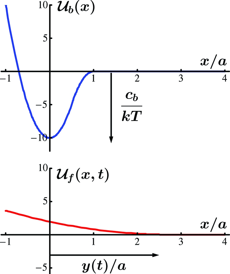
The interaction energy landscape (Upper) Typical bond energy profile characterized by a well depth cb with dimensions of energy and a width a with dimension of length. This profile is time-independent. (Lower) Force potential profile that is fixed in shape and translates in the x direction in a way prescribed by y(t).
In developing probabilistic models of the response of a molecular bond to force, a common approach has been to replace the Boltzmann factor e−b(x) with e−b(x)−fx/kT, where f is the instantaneous value of the force acting in the direction of x. But if the quantity of interest is the resisting force of the bond, then an approach based on describing the confinement of the bond state in terms of force is fraught with difficulty. Instead, we describe confinement in terms of a variable that is work-conjugate to force with respect to system energy. The external coordinate concept of Gibbs (10) provides the conceptual basis for doing so.
Loading is taken into account here by introducing a second energy profile, say f(x,t), which is fixed in shape but which translates in the x direction with respect to b(x). We assume that f(x,t) has a unique value defined by the condition f(y(t),t) = 0, which is satisfied identically in time for some position history y(t). The relative position can then be specified by the external coordinate y(t) as illustrated in the lower portion of Fig. 1. For example, if the total compliance of the molecules themselves and of the loading apparatus can be represented by an equivalent linear spring, then this profile would be parabolic with its apex corresponding to x = y(t) and with its curvature being the stiffness of the equivalent spring. In general, applied “loading” is prescribed through the deterministic coordinate y(t), thereby influencing the accessibility of states of the random variable. The total energy landscape or profile representing the system energy is the sum
This accounts for the compliance of all aspects of the configuration, including the molecules themselves as well as a loading apparatus.
State of the Bond.
A large ensemble of nominally identical systems under identical input y(t) is described by means of the probability density ρ(x,t); the value of ρ(x,t) is the probability of finding the system of interest in position x at time t. It is the evolution of this probability distribution for given y(t) that determines the survival probability R(t). Beginning with Kramers (2), a framework was established for describing the evolution of probability density ρ(x,t) for the case of a time-independent energy landscape. This general framework is adopted here, and it is generalized to account for the time dependence of the energy landscape. Denote the flux of states in the x direction at time t by j(x,t). Local conservation of states requires that
The associated transport equation follows from the constitutive assumption that the flux of states is proportional to the gradient in the local chemical potential, the latter being a feature of the underlying free-energy function for the system; see SI Appendix. In the present circumstances, the flux of states can be related to the probability distribution and the interaction energy field according to
where D is a diffusivity for the underlying diffusion process. Its value is not known a priori, and it joins cb and a as the third unknown characterizing parameter.
The corresponding force acting on the ensemble is then determined as the time-dependent quantity which is work conjugate to the external coordinate y(t) with respect to the free-energy function,
where the derivative appearing under the integral sign is the ordinary derivative of (x,t) with respect to y for fixed values of x and t. The extraction of f(t), exact within the thermodynamic framework, is described in the SI Appendix. Technically, the limits of integration are x1 → −∞ and x2 → ∞. However, the density is expected to be negligibly small at points far from the bond well compared with a and the integral expressions are expected to be convergent. Consequently, the limits of integration can be chosen to have finite magnitudes equal to several times a in either direction without introducing consequential error.
The expression 4 presumes that a large number of identical bonds are simultaneously subjected to the imposed constraint motion y(t) and that each individual bond responds independently of the response of any other bond in the ensemble. The quantity f(t) is then the total force acting on the ensemble divided by the number of bonds within the ensemble. As such, it is a statistical characteristic of all responses rather than a representation of the force on any particular bond. This distinction is relevant to the strategy adopted by Gaub and coworkers (11) in designing experiments to probe bond characteristics by deforming many noninteracting but nominally identical bonds simultaneously.
The Bond Survival Probability.
The survival probability of the bond R(t) is the fraction of bonds in the ensemble that remain intact at time t. In terms of the density of states, it is the fraction of bonds remaining within the interval x1 < x < x+(t) at time t,
where x+(t) identifies the location of the edge of the bond well as indicated in Fig. 2. The transport Eq. 3 is readily inverted to obtain an expression for ρ(x,t) in terms of j(x,t); see SI Appendix. Following Kramers (2), we assume that x2 is the point of no return for states diffusing away from the well, and we set ρ(x2,t) = 0. The inverse expression for ρ(x,t) in terms of j(x,t) is then
Fig. 2.

Time evolution of the energy landscape (x,t). The value f(0,t) is subtracted from each graph to keep the individual plots within a reasonable field of view. The locations of the local maximum and minimum of each curve are represented by x+(t) and x−(t), respectively, at any time t.
Integration of both sides of this equation over x1 < x < x+ leads to
The integrand of the inner integral on the right side of Eq. 7 has an exponential peak at ξ = x+(t). Likewise, the integrand of the outer integral has an exponential peak at x = x−(t), the position of the bottom of the well. Consequently, the double integral 7 is ideally suited for approximate evaluation by means of the Laplace method (12). Although this is an asymptotic method based on the presumption that cb is large compared with kT (the deep well assumption of Kramers), it is quite accurate for values of cb as small as 3 or 4 kT. The quality of the approximations is discussed in some detail below. Successive application of the Laplace method yields
 |
as an approximate expression for the survival probability; see SI Appendix. The quantity 11(x±,t) identifies the curvature of the landscape profile at point x = x±(t) at time t. The curvature at x = x+(t) is negative, necessitating use of the absolute value under the square root operator to properly represent the result of asymptotic evaluation.
The flux j(x,t) is not known a priori, but its value at x = x+(t) is precisely –Ṙ(t), the net rate at which states leave the bond well. If the factor of j(x+,t) in Eq. 8 is denoted by Koff(t)−1 then we obtain the rate equation
for the survival probability. We note that Koff(t) depends explicitly on features of the energy landscape, but is independent of the density of states. The solution of the differential equation 9 is
The force f(t) acting on the ensemble is defined in Eq. 4. If the expression for probability density ρ(x,t) in Eq. 6 is substituted into the expression for force and if the result is evaluated approximately by means of the asymptotic methods used above (see SI Appendix), it follows that
This approximate expression for force as the product of the survival probability R(t) times the most likely value of force for individual states within the well is simple and intuitive. The former factor accounts for the decrease in number of states within the well over time, whereas the latter factor reflects the increasingly severe confining influence of the constraint f(x,t). It is noted that no assumption has yet been made about the imposed motion y(t) that induces bond separation. In particular, the approximate forms of both survival probability in Eq. 10 and of ensemble force in Eq. 11 presume neither constant rate of imposed motion nor constant rate of applied force.
As shown in the foregoing development, the rate equation Eq. 9 follows directly from the Smoluchowski partial differential equation governing the probability distribution, which, in turn, is a consequence of an underlying thermodynamic free energy of the system at constant temperature. The constraint of constant temperature arises through the assumption that the debonding process evolves in a large isolated heat reservoir, with the energy drawn from the reservoir to stimulate diffusion being immediately returned through dissipation of the microscopic fluctuations. In the work of Hummer and Szabo (7) and Dudko et al. (9), the form of the first-order rate equation (Eq. 9) was assumed as the starting point for description of bond separation.
Results
To demonstrate the implications of the results in the preceding sections, representative choices for the features of the system are required. As a convenient form for the bond potential b(x), we adopt
 |
which is the expression that was used to generate Figs. 1 and 2. Numerical results are presented below for the integration range defined by x1 = −a and x2 = 5a, a range found to be adequate for the purpose.
For the loading potential f(x,t), we assume that the system compliance is that of a linear spring of stiffness κ in tension. If the loading system is incapable of exerting compressive force, then
The form of the term kT∂y(t)(x,t) appearing in the definition of force, Eq. 4, is simply κ(y(t) − x) in this case.
For the interaction potential function (x,t) defined in this way, the approximate description of the time dependence of the off-rate appearing in the rate equation (Eq. 9) takes the explicit form
 |
for arbitrary imposed motion of the constraint y(t). For a force equal to κy(t) and for cb ≫ aκ, the exponential factor in Eq. 14 reduces to the exponential factor in equation 3 of ref. 8 for ν = 1/2.
This result in Eq. 14 illustrates the significance of the relative magnitudes of two combinations of system parameters, one of which is time-dependent. The first of these parameters is 4cb + a2κ with value usually dominated by the bond strength cb. The second parameter is 2aκy(t), which is essentially 2a times the nominal force being transmitted to the bond itself through the combined effects of compliance of the loading train and the imposed remote constraint. Early in the loading process, the difference between these two parameters is dominated by the first parameter and, consequently, the off-rate is exponentially small. However, as time goes on, the value of y(t) increases continuously so that, eventually, the values of the two terms are comparable. When this happens, the exponent appearing in the expression for off-rate becomes relatively small and, consequently, the dependence of off-rate on time increases dramatically. Essentially, this is the transition reflected in the behavior of the survival probability with increasing time.
The off-rate factor appearing in Eq. 14 is expressed in terms of dimensional parameters representing physical quantities. However, these parameters can be gathered into dimensionless groups for various purposes. Commonly, we think of the values of κ, kT, and y(t) as being specified and the values of cb, a, and D as being inferred from observations. With this point of view, a convenient set of nondimensional parameters is , , and , where vy is a constant speed that is characteristic of y(t), possibly an initial speed or a maximum speed or an average speed, for example.
Constant Imposed Speed.
As a specific motion of the load point, we assume constant speed v > 0, starting at the root of the bond well at x = 0 at the time t = 0, so that
In this case, the expression for survival probability Eq. 10 can be evaluated explicitly in terms of the error function; the result is shown in the SI Appendix, where it is evident that the expression for R(t) exhibits the time dependence anticipated at the outset. As an illustration of its behavior, R(t) is evaluated for the parameter values
to produce the solid curve in Fig. 3.
Fig. 3.

Results of survival probability versus time. Comparison of the analytical result for bond R(t) with numerical simulation results for loading rate v = 1 (in nm/ms) and loading stiffness κ = 0.5 (in pN nm). The former is defined in Eq. 5 versus time t (in ms). The discrete points are determined by means of numerical solution of the equivalent boundary value problem for the Smoluchowski partial differential equation.
The expression for R(t) was obtained by application of approximate methods of analysis, so it is essential that the quality of the approximation should be examined. Because R(t) reflects a feature of the solution of the Smoluchowski partial differential equation for particular initial and boundary conditions, an appropriate basis for comparison is a full numerical solution of one and the same boundary value problem for that differential equation. This has been carried out by means of the numerical finite-element method for the same parameter values listed in Eq. 16 and results are indicated by means of discrete points in Fig. 3. The numerical procedure leads to discrete values of the probability distribution ρ(x,t) at 800 equally spaced values of x at discrete times t. At any particular time, the value of R(t) is extracted by numerical integration of the probability distribution over those spatial intervals included within the well x1 < x < x+(t).
In the asymptotic analysis, states were allowed to flow outward through x = x2. However, rather than assume that they virtually vanished in the finite-element simulation, these were collected in an energy reservoir beyond x = x2 that was added to the simulation for this purpose. This was done to verify that states are indeed conserved continuously in time. The integral of probability density, including states accumulated in this reservoir, was computed to be within 0.1% of the theoretical value of one for the entire time range of interest.
Calculation of the Mean Force.
A graph of f(t) versus t for constant speed constraint motion (Eq. 15), and with values of parameters as prescribed in Eq. 16, calculated according to the asymptotic expression (Eq. 11) for force obtained above, is shown in Fig. 4. The influence of the increase in time due to the increasing severity of the constraint imposed by the loading and the decrease in time due to the decreasing fraction of bonds remaining within the well is evident in the figure.
Fig. 4.

Mean force on a bond versus time. The solid line is a plot of the ensemble force f(t) (in pN) versus time t (in ms) according to Eq. 11 for the parameter values in Eq. 16. The discrete points show the results of a detailed numerical solution of the underlying boundary value problem for the Smoluchowski equation with the same parameter values. The dashed curve represents the force acting on an individual bond up to the instant of its separation.
For purposes of comparison, values of force at several discrete values of time have been extracted from the numerical solution of the boundary value problem according to the exact expression for force given in Eq. 4. The results are included as the discrete points appearing in Fig. 4. The force history is very well represented by the asymptotic approximation.
A novel experimental approach toward measuring molecular bond characteristics has been introduced by Gaub and coworkers (11). They measure the net force acting on many nominally identical bonds as they are separated simultaneously. Thus, the result measured is the mean force per bond f(t) across all bonds, both intact and separated, which differs from the actual force on a particular bond up to separation φ(t) = kTκ(vt − x−(t)), in general. To illustrate this point, the graph of φ(t) is included in Fig. 4. As is evident from the figure, the two representations of force are virtually identical as long as the survival probability is near one, but they diverge markedly as the survival probability approaches one-half. For the particular case illustrated in Fig. 4, the most likely force at separation is reached at time t ∼ 17 ms and, by this time, the difference between f(t) and φ(t) is significant.
Sample Force Probability Distributions.
As was noted in ref. 8, the probability that a particular bond subjected to a particular loading will separate at the force φ is related directly to the survival probability R(t). Suppose that this force probability distribution is denoted by P(φ), where the history of force acting on an individual bond is φ(t). For constant speed loading, the relationship between R(t) and P(φ) is
This distribution is readily calculated for any particular case, for example, the case defined by the parameter value set in Eq. 16.
Fig. 5 shows the probability distribution for this particular set of parameter values, as well as the corresponding distributions for larger and smaller values of loading speed v (with the other parameter values unchanged). In all cases, of course, the area under the curve is one. The influence of changing the value of loading stiffness κ to values smaller than or larger than the value included in the reference parameter set Eq. 16, while leaving other parameter values unchanged, is demonstrated in the SI Appendix. It is evident from the result that the loading apparatus stiffness also has a marked influence on response, as has been observed by Evans (14) and Walton et al. (15).
Fig. 5.

Probability distribution of separation force. The distribution of the probability P that a particular bond will separate at force φ for the parameter values in Eq. 16, along with several examples of this distribution for larger or smaller values of loading speed v.
An Illustration of Data Inversion.
The main purpose of the foregoing analysis is to gain insight into the connection between characterizing properties of a molecular bond and aspects of the response of the bond to controllable mechanical stimulus. Consequently, the prospect for using the results in the interpretation of experimental data is of interest.
Suppose that the graphs in Fig. 5 are viewed as “experimental data” for purposes of discussion in this section. We pretend that these “data” were generated with known values of the loading parameters v, κ, and kT but unknown values of bond-characterizing parameters. Then, we ask which values of cb, a, and D are implied by the theoretical description of survival probability R(t) given in Eq. 10 or the corresponding force probability P(φ) given in Eq. 17.
The separation force for each loading rate in Fig. 5 is identified by a particular value of φ, say φ*, corresponding to the local maximum in distribution P(φ). As shown in Eq. 11, the force φ(t) depends on time according to κ(vt − x−(t)) so that a unique time, say t*, is identified with φ* = φ(t*). The attainment of a maximum value in P(φ) occurs nearly (but not exactly) at the instant at which the survival probability R(t) has been reduced to the value one-half, that is, R(t*) ≈ 0.5. The latter seems to be the simplest form of an equation to be solved for the characterizing parameters.
A simple and seemingly stable solution procedure is as follows. Values of κ and kT are fixed, the value of v is fixed at one of the values represented in Fig. 5, and values of cb, a, and D are sought. It is evident that the equation R(t*) = 0.5 can be solved for D in terms of other parameters as
where A(cb,a,v) is the coefficient of D in the exponent of the expression defining R(t) in Eq. 10. Then, we plot level curves of D as defined by the right side of Eq. 18 in the plane spanned by coordinates cb and a for each of the values represented in Fig. 5 to be used in the inversion process. If a point in the plane at which all level curves for a particular value of D intersect then the coordinates of this point identify the values of cb and a underlying the “data.” The corresponding value of D is the value on these intersecting level curves, which completes the inversion process.
An illustration of such a contour plot is shown in Fig. 6. The region represented in the figure is spanned by the parameter ranges 0.5 < a < 1.5 (in nm) and 25 < cb < 55 (in pN nm). Level curves are shown for D = 0.1, 1, and 10, conveniently including the value we know to be correct in this case. It is evident that the level curves for D = 1 intersect at the point cb ≈ 40, a ≈ 1 which defines the values of the characterizing parameters being “sought.” An actual inversion of data will surely begin with a larger range of parameters in which to search for intersections, followed by several refinement steps; a more sophisticated strategy for deciding when a conjunction of contours actually occurs will also be needed to account for scatter in the data.
Fig. 6.

Level curves of diffusivity D in the plane of bond depth cb and bond well width a. The values of D are 0.1 (solid), 1 (short dashed), and 10 (long dashed). The common point represents the values of a and cb underlying the “data” on which the plots are based.
We note that in discussions of extracting these parameter values it has been common to use Kramers' off-rate for the undistorted bond b(x) rather than D as the rate parameter in the set to be determined (9, 11). However, this off-rate is determined by cb, a, and D together so this difference does not seem to be consequential.
Discussion
In this report, we have described an analysis that leads to an explicit relationship between the three parameters commonly thought to characterize the resistance of a molecular bond and an external mechanical force under constant rate conditions. The principal result is an expression for bond survival probability. Furthermore, an explicit expression for the time-dependent off-rate of a molecular bond for any imposed separation rate is given in Eq. 14. These results are obtained by asymptotic approximation of an integral representation of the solution of the underlying Smoluchowski partial differential equation, and the quality of the approximation has been confirmed by comparison of its implications with an accurate numerical solution of the corresponding full boundary value problem for the Smoluchowski equation. Finally, a means of extracting actual values of characterizing parameters from experimental data has been suggested for data presented in the form of a measured force probability distribution as introduced by Evans and Ritchie (1). Our hope is that readers will also find the way in which force is handled within the statistical development to be more versatile than are some of the other treatments that have appeared in the literature.
Still, there are several lingering questions on which we include a few observations. For one thing, the main results have been obtained on the basis of a particular energy landscape (x,t). Naturally, this raises a question about the generality of the conclusions. Quantitatively, we have pursued this matter by carrying out detailed numerical analyses of the boundary value problems for the Smoluchowski equation for several energy landscapes, which differ in detail, but which are based on the same values of well depth, well width, and diffusivity. The results have shown relatively minor variation from case to case. Furthermore, we have carried out an asymptotic evaluation for an angular energy landscape composed of three straight lines but the same values of well depth and width. Even this extreme shape led to an expected value of separation force only 10% larger then for the interaction potential used here. We have no particular concerns on this point, but the matter requires more thorough study.
When considered from another point of view, there is little basis on which to pursue the question. It is possible to extract survival probability versus time for any one-dimensional interaction energy proposed. However, with the current level of understanding of the experimental data on the bond characteristics, there is no basis for discriminating among the results obtained. When more refined data become available on molecular bond separation, it will likely lead to further study of details of the shape of the interaction potential beyond depth, width, and a rate coefficient.
A second point concerns the quality of the asymptotic approximation scheme used here. Strictly speaking, the results are correct asymptotically in the limit as cb/kT → ∞, but this is not a useful statement on the range of validity of the approximation. Kramers (2) presented the asymptotic limits of his result for off-rate as the principal result of his work, and the literature is replete with suggestions that the asymptotic description and the implied restriction to “deep” wells is somehow too restrictive.
To develop a sense of the range of validity of this approximation, we considered the integral defining the survival probability in Eq. 7 but with the factor j(ξ,t)/D set equal to one. As such, the integral retains precisely those features of the expression that suggest asymptotic evaluation as a useful approach for its approximation. The asymptotic approximation of this integral appears on the right side of Eq. 8 with j(x+,t)/D set equal to one. For parameter ranges of interest here, the asymptotic approximation is found to be virtually indistinguishable from the results of accurate numerical evaluation for values of cb/kT greater than about 5, and to be useful approximations for the values of cb/kT as small as 2 or 3. These results are illustrated graphically in the SI Appendix. Consequently, we believe that the fidelity of the asymptotically derived results is high for a range of system parameter values sufficiently broad to include most observations.
Supplementary Material
Acknowledgments.
We thank Olga Dudko, Rob Phillips, and Ana Smith for helpful suggestions and observations on the details of the presentation. This work was supported by the Materials Research Science and Engineering Centers Program of the National Science Foundation at Brown University, Award DMR-0520651.
Footnotes
The authors declare no conflict of interest.
See Commentary on page 8795.
This article contains supporting information online at www.pnas.org/cgi/content/full/0903003106/DCSupplemental.
References
- 1.Evans E, Ritchie K. Dynamic strength of molecular adhesion bonds. Biophys J. 1997;72:1541–1555. doi: 10.1016/S0006-3495(97)78802-7. [DOI] [PMC free article] [PubMed] [Google Scholar]
- 2.Kramers HA. Brownian motion in the field of force and the diffusion model of chemical reactions. Physica. 1940;7:284–304. [Google Scholar]
- 3.Risken H. The Fokker-Planck Equation. 2nd Ed. Berlin: Springer; 1989. [Google Scholar]
- 4.Hanggi P, Talkner P, Borkovec M. Reaction-rate theory: 50 years after Kramers. Rev Mod Phys. 1990;62:251–342. [Google Scholar]
- 5.Chandrasekhar S. Stochastic problems in physics and astronomy. Rev Mod Phys. 1943;15:1–89. [Google Scholar]
- 6.Bell GI. Models for the specific adhesion of cells to cells. Science. 1978;200:618–627. doi: 10.1126/science.347575. [DOI] [PubMed] [Google Scholar]
- 7.Hummer G, Szabo A. Kinetics from nonequilibrium single-molecule pulling experiments. Biophys J. 2003;85:5–15. doi: 10.1016/S0006-3495(03)74449-X. [DOI] [PMC free article] [PubMed] [Google Scholar]
- 8.Dudko OK, Hummer G, Szabo A. Intrinsic rates and activation free energies from single-molecule pulling experiments. Phys Rev Lett. 2006;96:108101. doi: 10.1103/PhysRevLett.96.108101. [DOI] [PubMed] [Google Scholar]
- 9.Dudko OK, Hummer G, Szabo A. Theory, analysis, and interpretation of single-molecule force spectroscopy experiments. Proc Natl Acad Sci USA. 2008;105:15755–15760. doi: 10.1073/pnas.0806085105. [DOI] [PMC free article] [PubMed] [Google Scholar]
- 10.Gibbs JW. Elementary Principles in Statistical Mechanics. New York: Dover Publications; 1960. (originally published by Yale Univ Press, 1902) [Google Scholar]
- 11.Neubet G, Albrecht CH, Gaub HE. Predicting the rupture probabilities of molecular bonds in series. Biophys J. 2007;93:1512–1223. doi: 10.1529/biophysj.106.100511. [DOI] [PMC free article] [PubMed] [Google Scholar]
- 12.Ablowitz MJ, Fokas AS. Complex Variables. 2nd Ed. Cambridge, UK: Cambridge Univ Press; 2003. pp. 430–438. [Google Scholar]
- 13.Marshall BT, et al. Measuring molecular elasticity by atomic force microscope cantilever fluctuations. Biophys J. 2006;90:681–692. doi: 10.1529/biophysj.105.061010. [DOI] [PMC free article] [PubMed] [Google Scholar]
- 14.Evans E. Probing the relation between force–lifetime–and chemistry in single molecular bonds. Annu Rev Biophys Biomol Struct. 2001;30:105–128. doi: 10.1146/annurev.biophys.30.1.105. [DOI] [PubMed] [Google Scholar]
- 15.Walton EB, Lee S, Van Vliet KJ. Extending Bell's model: How force transducer stiffness alters measured unbinding forces and kinetics of molecular complexes. Biophys J. 2008;94:2621–2630. doi: 10.1529/biophysj.107.114454. [DOI] [PMC free article] [PubMed] [Google Scholar]
Associated Data
This section collects any data citations, data availability statements, or supplementary materials included in this article.