Predictions of RNA secondary structure by combining homologous sequence information

Abstract

Motivation: Secondary structure prediction of RNA sequences is an important problem. There have been progresses in this area, but the accuracy of prediction from an RNA sequence is still limited. In many cases, however, homologous RNA sequences are available with the target RNA sequence whose secondary structure is to be predicted.

Results: In this article, we propose a new method for secondary structure predictions of individual RNA sequences by taking the information of their homologous sequences into account without assuming the common secondary structure of the entire sequences. The proposed method is based on posterior decoding techniques, which consider all the suboptimal secondary structures of the target and homologous sequences and all the suboptimal alignments between the target sequence and each of the homologous sequences. In our computational experiments, the proposed method provides better predictions than those performed only on the basis of the formation of individual RNA sequences and those performed by using methods for predicting the common secondary structure of the homologous sequences. Remarkably, we found that the common secondary predictions sometimes give worse predictions for the secondary structure of a target sequence than the predictions from the individual target sequence, while the proposed method always gives good predictions for the secondary structure of target sequences in all tested cases.

Availability: Supporting information and software are available online at: http://www.ncrna.org/software/centroidfold/ismb2009/.

Contact: hamada-michiaki@aist.go.jp

Supplementary information:Supplementary data are available at Bioinformatics online.

1 INTRODUCTION

Secondary structure prediction of RNA sequences is one of the most important fundamental problems in biological sequence information analysis. The importance of accurate predictions has increased due to the recent findings in functional non-coding RNAs. Although a number of algorithms and tools have been developed for this problem (e.g. Andronescu et al., 2007; Do et al., 2006a; Hamada et al., 2008; Hofacker et al., 1994; Parisien and Major, 2008), their accuracies are limited. In real cases, however, it is expected that the accuracies can be improved by taking into account the information of RNA sequences that are homologous to the target RNA sequence whose secondary structure is to be predicted. There have been proposed several methods with this respect (e.g. Hamada et al., 2006; Hofacker et al., 2002; Kiryu et al., 2007b).

The problem targeted by this article is defined as follows.

Problem 1. —

Given a single RNA sequence x and a set of its homologous sequences D, predict a secondary structure of x using the information of D.

It is assumed that x and each sequence x′ in D share a common secondary structure, and the secondary structure of x is predicted by combining information present in D. This problem can be solved by mapping the predicted common structure of the entire sequences to the target sequence as follows: (i) compute a multiple alignment A for the set of sequences D∪{x} (e.g. Do et al., 2005, 2008; Tabei et al., 2008), (ii) predict a common secondary structure of A (e.g. Bernhart et al., 2008; Hamada et al., 2008; Seemann et al., 2008) and (iii) predict a secondary structure of x by mapping the predicted common secondary structure to the target RNA sequence x. The obtained secondary structures are more reliable in general than the predictions only from individual sequences. There are problems in the above approach, however, because the secondary structures of individual sequences are not exactly the same as the common secondary structure and the quality of the multiple alignment strongly influences the performance of the prediction.

In this article, we propose a novel estimator for Problem 1 which yields a direct prediction of the secondary structure of x by combining the information of the homologous sequences D without assuming the multiple alignment or the common structure of the entire sequences (Fig. 1). The proposed method models the probabilistic distribution of the pairwise common structure between the target RNA sequence and each homologous sequence, and maximizes the expected accuracy of the prediction of the target RNA sequence under the combined probabilistic distribution. The expectation is calculated under all the suboptimal secondary structures of the target sequence and under all the suboptimal pairwise alignments of the target sequence and its homologous sequences using posterior decoding method, which is based on a posteriori probabilities such as base-pairing probabilities of RNA or match probabilities of alignment and has been successfully applied in bioinformatics (Bradley et al., 2008; Carvalho and Lawrence, 2008; Ding et al., 2005; Fariselli et al., 2005; Holmes and Durbin, 1998; Lunter et al., 2008; Miyazawa, 1995; Paten et al., 2009; Wong et al., 2008). In secondary structure prediction of RNA, posterior decoding methods are used in the maximum expected accuracy (MEA) estimator of CONTRAfold (Do et al., 2006a), the centroid estimator (Carvalho and Lawrence, 2008; Ding et al., 2005) and the γ-centroid estimator of CentroidFold (Hamada et al., 2008). We demonstrate that the prediction accuracy of the proposed method outperforms that of conventional secondary structure prediction methods.

Fig. 1.

A schematic diagram of our proposed method and other existing methods (M1, M2, M3) for Problem 1. See Section 3.2 for precise descriptions of M1, M2 and M3.

2 METHODS

2.1 Discrete spaces and probability distributions

In this article, the following discrete spaces and probability distributions on those spaces play important roles in order to define proposed estimators.

2.1.1 A space of secondary structures: 𝒮(x)

A secondary structure of an RNA sequence x is represented as an upper triangular binary matrix θ = {θ_ij}_i<j, where the (i, j) element θ_ij of the matrix θ is equal to 1 if x_i and x_j form a base pair and to 0 if x_i and x_j do not form a base pair (Fig. 2). A consistent secondary structure represented by θ should satisfy the following constraints: (i) ∑_i<jθ_ij+∑_j<iθ_ji≤1 for any j (each position in a sequence is allowed to form a base pair with one other base at most), and (ii) θ_ij+θ_kl≤1 for any i < k < j < l (the formation of any two base pairs which results in a pseudo-knot is not allowed). We denote with 𝒮(x) the space of all secondary structures θ of an RNA sequence x. Note that to predict the secondary structure of x is equivalent to predicting a point θ in 𝒮(x). We obtain a probability distribution p^(s)(·|x) on 𝒮(x) by using the McCaskill model (McCaskill, 1990), the CONTRAfold model (Do et al., 2006a), the Simfold model (Andronescu et al., 2007) and the SCFG model (Dowell and Eddy, 2004). By using the distributions, a base-pairing probability p^(s,x)_ij, which is the probability with which x_i and x_j form a base pair, is computed as p_ij^(s,x) = p^(s)(θ_ij=1|x) = ∑_θ∈S(x)I(θ_ij = 1)p^(s)(θ|x), where I(·) is the indicator function, which takes a value of 1 or 0 depending on whether the condition constituting its argument is true or false. We refer to {p_ij^(s,x)}_i<j as a base pairing probability matrix, which can be computed by using the inside–outside algorithm (e.g. McCaskill, 1990), whose time complexity is O(|x|³) where |x| is the length of x.

Fig. 2.

Representation of a secondary structure of an RNA sequence.

2.1.2 A space of pairwise alignments: 𝒜(x, x′)

Similarly to the secondary structure of an RNA sequence, a pairwise alignment of two sequences x and x′ (e.g. DNA sequences, RNA sequences or amino acid sequences) is represented as a binary matrix θ={θ_ik}_i,k, where θ_ik=1 if x_i is aligned with x′_k and θ_ik=0 if x_i is not aligned with x′_k (Fig. 3). A consistent alignment represented by θ should satisfy the following constraints: (i) ∑_k θ_ik ≤ 1 for any i, (ii) ∑_iθ_ik ≤ 1 for any k, (iii) θ_ik+θ_jl≤1 for any i<j and l<k. In this article, the space of all pairwise alignments of x and x′ is denoted by 𝒜(x, x′). We can obtain the probability distribution p^(a)(θ|x, x′) on 𝒜(x, x′) by using the PHMM model (Durbin et al., 1998), the Miyazawa model (Miyazawa, 1995), the ProbAlign model (Roshan and Livesay, 2006), the CONTRAlign model (Do et al., 2006b). By using the distributions, the alignment match probability p^(a,x,x′)_ik, which is the probability that x_i is aligned with x′_k, is computed as p_ik^(a,x,x′) = p^(a)(θ_ik = 1|x, x′) = ∑_{θ∈𝒜(x,x′)}I(θ_ik = 1)p(θ|x, x′). We refer to {p_ik^(a,x,x′)}_i,k as an alignment match probability matrix, which can be computed by using the forward–backward algorithm (Durbin et al., 1998), whose time complexity is O(|x‖x′|). Moreover, the joint probability p^(a,x,x′)_ik,jl, which is the probability that x_i is aligned with x′_k and x_j is aligned with x′_l, is also computed as p^(a,x,x′)_ik,jl=p^(a)(θ_ik = 1, θ_jl = 1|x, x′) = ∑_{θ∈𝒜(x,x′)}I(θ_ik = 1)I(θ_jl = 1)p^(a)(θ|x, x′). Note that {p^(a,x,x′)_ik,jl}_i<j,k<l can be computed by using a variant of the forward–backward algorithm whose time complexity is equal to O(|x|²|x′|²).

Fig. 3.

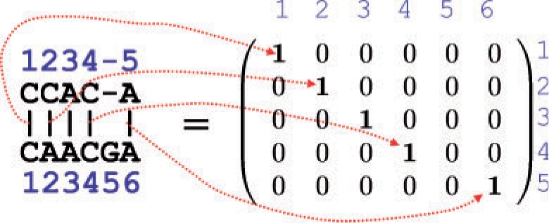
Representation of a pairwise alignment of two RNA sequences.

2.1.3 A space of structural pairwise alignments of RNA sequences: 𝒮𝒜(x, x′)

A structural alignment (e.g. Kiryu et al., 2007a; Sankoff, 1985) of two RNA sequences x and x′ is represented as θ = {θ_ijkl^(p)}_i<j,k<l × {θ_uv^(l)}_u,v where θ_ijkl^(p) = 1 if a base pair (x_i, x_j) in x is aligned with a base pair (x′_k, x′_l) in x′ and θ_uv^(l) = 1 if x_u in a loop region of x is aligned with x_v′ in a loop region of x′ (Fig. 4). In accordance with a consistent structural alignment, each element in θ cannot take an arbitrary value in {0, 1}, where θ satisfies several conditions. Moreover, a space of structural alignments of two RNA sequences x and x′ is denoted as 𝒮𝒜(x, x′). We obtain a probability distribution p^(sa)(θ|x, x′) by the pair SCFG model, the Sankoff model (Sankoff, 1985). We also denote a probability that a base pair (x_i, x_j) in x is aligned with a base pair (x′_k, x′_l) in x′ as p_ijkl^{(sa,p,x,x′)} = p^(sa)(θ_ijkl^(p) = 1|x, x′). Note that {p_ijkl^{(sa,p,x,x′)}}_i<j,k<l can be computed by using a variant of the inside–outside algorithm of the Sankoff model (Sankoff, 1985), whose time complexity is O(|x|³|x′|³).

Fig. 4.

Representation of a structural alignment of two RNA sequences.

2.2 Designing estimators for Problem 1

Most of the existing decoding methods are regarded as the following estimators (e.g. Carvalho and Lawrence, 2008; Hamada et al., 2008): if Y is a space from which we would like to obtain a prediction, referred to as a predictive space, Θ is a space which is referred to as a parameter space and is potentially different from the predictive space, p(θ|d) is a probability distribution on the parameter space Θ given a dataset d, and G(θ, y) is a gain function between Θ and Y, then an estimator on the predictive space is defined as

(1)

(cf. Ding et al., 2005; Do et al., 2006a; Hamada et al., 2008; Kiryu et al., 2007b). Here, we can design a superior estimator by defining the gain function and the parameter space appropriately. For example, (Hamada et al., 2008) have proposed an estimator which maximizes the expectation α₁TP + α₂TN − α₃ FN − α₄FN (α_n > 0, n = 1, 2, 3, 4) with respect to a probability distribution on 𝒮(x), and confirmed that their estimators are superior to the MEA estimator used in CONTRAfold (Do et al., 2006a). Regarding Problem 1, we would like to predict the secondary structure of x so that the predictive space Y is 𝒮(x). Therefore, it is necessary to define the parameter space Θ and the probability distribution p(θ|x) on the parameter space Θ. In the following sections, we introduce several estimators: an estimator with less heuristics, and its approximations with some heuristics.

2.2.1 Estimator 1

Our assumption in Problem 1 is that x and every x′ ∈ D share a common secondary structure. The common secondary structure is naturally represented as a structural alignment of x and x′ (See Section 2.1.3). Therefore, we set the parameter space as Θ⁽¹⁾ = ∏_x′∈D𝒮𝒜(x, x′) and the probability distribution on Θ⁽¹⁾ as p⁽¹⁾(θ|x, D) = ∏_x′∈Dp^(sa)(θ^xx′|x, x′) for θ = ∏_x′∈Dθ^xx′∈∏_x′∈D𝒮𝒜(x, x′), where θ^xx′ is a structural alignment of x and x′ (i.e. θ^xx′∈𝒮𝒜(x, x′)). Moreover, the gain function is defined by

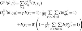for a prediction y ∈ 𝒮(x), where |D| denotes with the number of sequences in D and γ > 0 is a parameter which adjusts the Sensitivity and the positive predictive values (PPV) (see Section 3 for definition) of a predicted secondary structure. In this gain function, 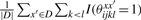is equal to the averaged number of a pair (x_i, x_j) which forms a base pair in the set of structural alignments {θ^xx′}_x′∈D and 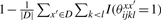is equal to the averaged number of a pair (x_i, x_j) which does not form a base pair in the set. Hence, the more base pairs (x_i, x_j) there exist in the set of structural alignments, the more gain in the gain function is given for the prediction y_ij = 1. Then, we define the estimator which maximizes the expectation of the gain function G⁽¹⁾(θ, y) on the probability distribution p⁽¹⁾(θ|x, D) as

(2)

It is clear that the estimator is equivalent to the γ-centroid estimator (Hamada et al., 2008) on 𝒮(x) when the probability distribution is defined by , where Φ is the natural map from a structural alignment θ′ ∈ 𝒮𝒜(x, x′) to the secondary structure θ ∈ 𝒮(x). The optimal secondary structure is computed by a Nussinov-type dynamic programming (Nussinov et al., 1978) as follows:

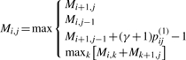(3)

where 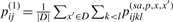. As described in Section 2.1.3, the time complexity to obtain {p^{(sa,p,x,x′)}_ijkl}_i<j,k<l is O(|x|³|x′|³), so it requires O(|D‖x|³ max_x′∈D|x′|³) time for computing {p_ij⁽¹⁾}_i<j. O(|x|³) time is required for the dynamic programming (3) in the case of {p_ij⁽¹⁾}_i<j. Therefore, the total time complexity is O(|D‖x|³ max_x′∈D|x′|³). This computational cost is too large to implement a practical application, so we approximate the estimator in the following sections.

2.2.2 Estimator 2

Since 𝒮𝒜(x, x′) and a probability distribution on the space require huge computational cost as noted in the previous section, we replace the parameter space Θ⁽¹⁾ and the gain function G⁽¹⁾(θ, y) by their approximations with some heuristics. The parameter space is approximated by the factorization of Θ⁽¹⁾ such as Θ⁽²⁾ = 𝒮(x) × ∏_x′∈D[𝒜(x, x′) × 𝒮(x′)] and the corresponding probability distribution on Θ⁽²⁾ is defined as

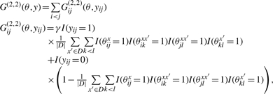
for θ = θ^x × ∏_x′∈D[θ^xx′ × θ^x′] ∈ Θ⁽²⁾, where θ^x ∈ 𝒮(x), θ^xx′ ∈ 𝒜(x, x′) and θ^x′ ∈ 𝒮(x′). We also consider two kinds of approximations of ∑_k<lI(θ_ijkl^xx′ = 1) in the gain function G⁽¹⁾(θ, y) as follows:

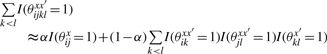where α ∈ [0, 1] is a weight parameter between the target sequence x and x′ ∈ D. An intuitive description of the difference in the two approximations is shown in Figure 5. The new gain functions are represented as

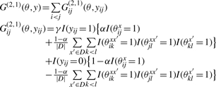and

respectively. Then, we introduce two estimators in order to maximize the expectation of G^(2,1)(θ, y) or G^(2,2)(θ, y) under the probability distribution p⁽²⁾(θ|x, D). We can obtain the secondary structure of each estimator by replacing p_ij⁽¹⁾ with

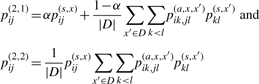in Equation (3), respectively. We refer to these two estimators as ‘appro2-1’ and ‘appro2-2’, respectively. As described in Section 2.1.2, time complexity for computing {p_iu,jv^(a,x,x′)} is O(|x|²|x′|²), and the cost is O(|D‖x|² max_x′∈D |x′|²) for obtaining {p_ij^(2,1)}_i<j or {p_ij^(2,2)}_i<j. This computational cost is still too large for calculating secondary structures whose length is more than several hundred bases. Therefore, we approximate this estimator in an attempt to reduce the computational cost.

Fig. 5.

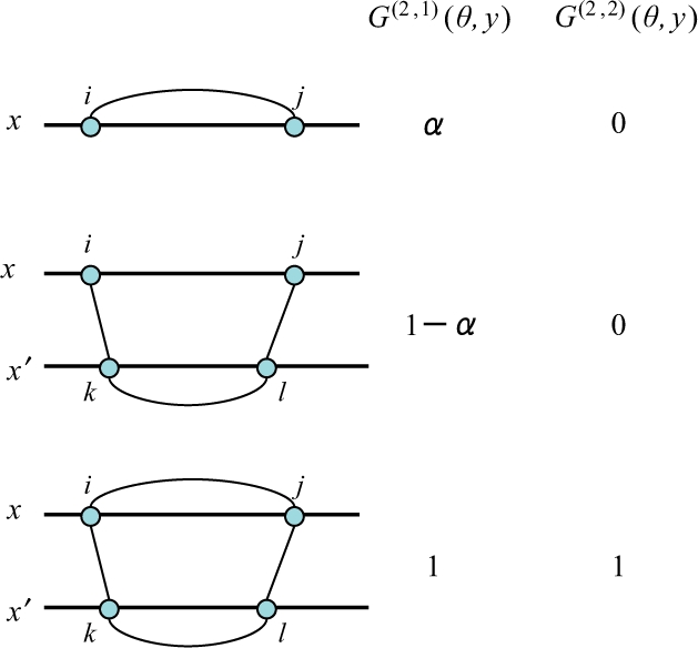
The difference between two gain functions G^(2,1)(θ, y) and G^(2,2)(θ, y). Each row indicates a configuration of θ on the target sequence x and each homologous sequence x′, and its positive contributions to the gain functions for y_ij = 1. For example, the middle row means that the configuration of θ_ij^x = 0 and θ_ik^xx′ = θ_kl^x′ = θ_jl^xx′ = 1 have a positive (1 − α) contribution for y_ij = 1 in the gain function G^(2,1), while have no contribution in the gain function G^(2,2).

2.2.3 Estimator 3 (proposed estimator)

By approximating p_ik,jl^(a,x,x′) to p_ik^(a,x,x′)p_jl^(a,x,x′), we replace p_ij^(2,1) and p_ij^(2,2) in the previous section by

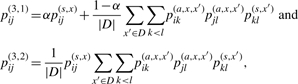respectively. Note that p_ij^(3,1) and p_ij^(3,2) take a value between 0 and 1, although they are not probabilities (more precisely, {p_ij^(3,1)}_i<j cannot be obtained by any probability distribution on 𝒮(x)). We refer to these two estimators as ‘appro3-1’ and ‘appro3-2’, respectively. If α = 1/(|D| + 1), {p_ij^(3,1)}_i<j is the same as a probabilistic consistency transformation of the base pairing probability matrix in Kiryu et al. (2007a). Even if we employ these approximations, the time complexity to obtain {p_ij^(3,1)}_i<j or {p_ij^(3,2)}_i<j still remains O(|D‖x|² max_x′∈D|x′|²). However, since the number of base pairs (x_k′, x_l′) in x′ where p_kl^(s,x′) > δ for a threshold δ is regarded as O(c|x′|) for a constant c, {p_ij^(3,1)}_i<j and {p_ij^(3,2)}_i<j can be computed by O(c|D‖x|² max_x′∈D|x′|) only if we sum through the base pairs (x′_k, x′_l) where p_kl^(s,x′) > δ in the equation p_ij^(3,1) and p_ij^(3,2). By definition, we see that the proposed estimators consider all suboptimal secondary structures of the target RNA sequence (and its homologous sequences) and all suboptimal pairwise alignments between the target sequence and each of homologous sequences. The proposed estimators have three parameters, α, γ and δ: the parameter α of the estimator appro3-1 represents the weight of the target sequence relative to its homologous sequences; γ is the parameter that strikes the balance between the sensitivity and specificity of the predictions; and δ represents the probability cutoff that influences the speed and accuracy of the algorithm. In Section 3.3, we confirm the relation between these parameters and prediction performance, and decide to set α = 1/(1 + |D|) and δ = 0.01 as default parameters.

3 EXPERIMENTS

We conducted all experiments in this section on our linux cluster machines, each of which has 2 GHz CPU of AMD Opteron(tm) Processor 246 and 4 GB memory. The accuracy of predicted secondary structures was evaluated through the following standard evaluation measures: Sensitivity = TP/(TP + FN) and PPV = TP/(TP + FP), where TP is the number of correctly predicted base pairs, FN is the number of base pairs in the reference structure that were not predicted and FP is the number of incorrectly predicted base-pairs. In all the figures described below, we plot the curve at γ ∈ {2^k : −5 ≤ k ≤ 10, k ∈ ℤ} ∪ {6} for the proposed estimators, the averaged γ-centroid estimators and the γ-centroid estimators (Hamada et al., 2008), which are implemented in the CentroidFold software.

3.1 Dataset

We used three datasets in our experiments. A summary of our datasets is described in Table 1.

Table 1.

Summary of dataset used in our experiments

	dataset1	dataset2	dataset3
#data	850	1547	215
#homo.seqs |D|	9	2–20	2–20
Length of seqs	48–389	50–500	500–1500
Source	Kiryu et al. (2007b)	Andronescu et al. (2008)	Andronescu et al. (2008)

#data means the number of test data which contains a target sequence and several homologous sequences. #hom.seq means the number of homologous sequence included in each test data. See Section 3.1 for details of each dataset.

3.1.1 The dataset1

We created a dataset called ‘dataset1’ by utilizing the dataset in Kiryu et al. (2007b) which contains 85 reference alignments of 10 sequences taken from 17 RNA families in the Rfam database (Griffiths-Jones et al., 2005) as follows: we selected each RNA sequence in each alignment in the Kiryu's dataset as a target sequence x and the other sequences in the alignment as homologous sequences D. The reference structure of the target sequence x is given by mapping the consensus structure in the alignment to the target sequence. As a result, we obtained 850 test data, each of which contains a target sequence and nine homologous sequences. Note that the dataset in Kiryu et al. (2007b) contained only the manually curated seed alignments with the consensus structures published in literature.

3.1.2 The dataset2 and dataset3

We created dataset called ‘dataset2’ and ‘dataset3’ from the RNA STRAND database (Andronescu et al., 2008), which contains manually curated RNA secondary structures of any type and organism. We selected reference secondary structures of target sequences out of 3704 non-redundant entries in the database, which satisfy all of the following conditions: (i) containing one molecule, (ii) not containing any ambiguous characters (i.e. any characters excluding A, U, G, C and T) (iii) not included in the family type ‘Other *’, ‘Synthetic RNA’ and ‘Unknown’ and (iv) whose length is more than 50 (500) nt and less than or equal to 500 (1500) nt for the dataset2 (the dataset3, respectively). We also created homologous sequences D of the target sequence by randomly selecting 2–20 sequences in the same family of the target sequence. As a result, the numbers of test data in the dataset2 and the dataset3 are 1547 and 215, respectively.

3.2 Compared methods

In the following sections, we compared the proposed method with three types of methods (Fig. 1) for Problem 1 as follows. Note that the default parameters were used in each tool unless the parameters were specified. (M1) Predict a secondary structure of a target RNA sequence x without using homologous sequence information. In this method, we used the tools of secondary structure prediction from an individual RNA sequence: RNAfold version 1.8.1 (Hofacker et al., 1994), SimFold in MultiRNAFold-1.11 with the ISMB 2007 best parameters (Andronescu et al., 2007) and CentroidFold version 0.0.4 (Hamada et al., 2008) with the CONTRAfold model (Do et al., 2006a), which is theoretically and experimentally superior to CONTRAfold itself. (M2) Align {x} ∪ D and predict a common secondary structure of the predicted multiple alignment, and then mapped the common secondary structure to the target sequence x. In this method, we used the tools of the multiple alignment of RNA sequences: ProbCons (RNA) (Do et al., 2005), RAF v1.00 (Do et al., 2008), MXSCARNA version 2 (Tabei et al., 2008) and the tools of the common secondary structure prediction from multiple alignments of RNA sequences: PETfold v1.0 (Seemann et al., 2008), RNAalifold version 1.8.1 (Bernhart et al., 2008) which was recently updated, and CentroidFold version 0.0.4 (Hamada et al., 2008) with the CONTRAfold model which implemented the averaged γ-centroid estimators. (M3) Simultaneously align and fold {x}∪D, and map the common secondary structure on the structural multiple alignment to the target sequence x. We used RAF v1.00 (Do et al., 2008) in this method. Note that this method can calculate the most likely structural alignment and its common secondary structure, sacrificing extremely huge computational time compared with M1, M2 and the proposed method.

3.3 Comparison within proposed methods

In this section, we mainly evaluated the performance of the proposed estimators with the various probabilistic models of p^(s) and p^(a), and the various parameters in the proposed method. We used the probability distribution p^(s)(·) on 𝒮(x) for an RNA sequence x in the McCaskill model (McCaskill, 1990) and the CONTRAfold model (Do et al., 2006a), and also used the probability distribution p^(a)(·) on 𝒜(x, x′) for two RNA sequences x and x′ in the ProbCons model (Do et al., 2005) and the ProbAlign model (Roshan and Livesay, 2006). Note that the fixed alignment is not required in the proposed method, while the method (M2) requires fixed alignments.

First, we aimed at determining the influence of the parameters α (which is used only in appro3-1) and δ in the proposed estimators on the dataset1. Figure 6a and Supplementary Figure S1 show the results of various α parameter when we set δ = 0. These show the suitability of α parameter in the appro3-1 for around 0.1, which is equal to α = 1/(|D| + 1) where |D| = 9 in this experiment since each test data in dataset1 contains nine homologous sequences. This suggests that the same weight between the target RNA sequence x and each sequence in D provided good prediction performance, and it seems to be a natural result. We also investigated the influence of the parameter δ described in Section 2.2.3. As shown in the Figure 6b (also see Supplementary Figs S2 and S3) in the case that δ < 0.01, the performance is almost the same as that of δ = 0. On the other hand, the total calculation times of the proposed estimator δ = 0.01 are much faster than that of δ = 0 (Table 2). Therefore, we decided to use α = 1/(|D| + 1) = 0.1 and δ = 0.01 in next experiments.

Fig. 6.

Performance of the different parameters for appro3-1. (a) We tested various values of α for δ = 0. (b) We tested various values of δ for α = 1/(|D| + 1) = 0.1. In both figures, we used p^(a) in the ProbCons model and p^(s) in the CONTRAfold model. The performance of the other combinations of probability distributions is shown in the Supplementary Material (Figs S1–S3).

Table 2.

Total calculation time in seconds (predicting secondary structures for 17 γ values of 850 RNA sequences) of the estimator appro3-1 for each δ and each combination of the probability distributions

δ	pa-ct	pa-mc	pc-ct	pc-mc
0	276 869	290 579	274 758	290 174
0.0001	16 471	5107	16 393	5009
0.001	7962	3202	7897	3124
0.01	3836	2130	3781	2065
0.1	2552	1600	2502	1541

We set α = 1/(|D| + 1) = 0.1 in this experiment. ‘x-y’ means appro3-1 with x of p^(a) and y of p^(s). pa, pc, mc and ct denote the ProbAlign model (Roshan and Livesay, 2006), the ProbCons model (Do et al., 2005), the McCaskill model (McCaskill, 1990) and the CONTRAfold model (Do et al., 2006a), respectively.

Second, we conducted an experiment for comparing appro3-1 and appro3-2 as described in Section 2.2.3. As shown in Figure 7a, appro3-1 outperformed appro3-2 under the same conditions (i.e. probability distributions p^(a) and p^(s)). We can observe that the best combination of the proposed estimators and the probability distributions is appro3-1 with the CONTRAfold model and the ProbCons model. Moreover, in order to examine the difference in performance of appro2-1 as described in Section 2.2.2 and appro3-1 as described in Section 2.2.3, we implemented the variant of the forward–backward algorithm for computing {p^(a,x,x′)_ik,jl}_i<j,k<l in the ProbCons model (Do et al., 2005). Figure 7b shows that appro3-1 provided almost the same performance as appro2-1, indicating that the approximation used in Section 2.2.3 does not influence the performance at all.

Fig. 7.

(a) The comparison of appro3-1 and appro3-2 for various combinations of p^(s) and p^(a). (b) The comparison of appro2-1 and appro3-1 in the ProbCons model (Do et al., 2005). Proposed-A-B (C) means the proposed estimator C (appro3-1, appro3-2, appro2-1 and appro2-2) with the model A [the McCaskill (McCaskill, 1990) model or the CONTRAfold model (Do et al., 2006a); this is a probability distribution on 𝒮(x)] and the model B [the ProbCons model (Do et al., 2005) or the ProbAlign model (Roshan and Livesay, 2006); this is a probability distribution on 𝒜(x, x′)].

3.4 Comparison with the other methods

In this section, we compared the proposed estimator with the other existing methods described in Section 3.2. For our method, we chose ‘appro3-1 with the CONTRAfold model and the ProbCons model for α = 1/(1 + |D|) and δ = 0.01’ (|D| is the number of homologous sequences), which achieved the best performance in the above experiments in several combinations of estimators, p^(s) and p^(a). This combination is denoted with the ‘proposed’ method below. First, we conducted an experiment on the dataset1 (see Section 3.1.1), which was also used in the previous section, and the result is shown in Figure S4 in the Supplementary Material. This result shows that the proposed method is better or comparable performance compared with the method (M1), (M2) and (M3). In this experiment, however, someone may be concerned about the over-fitting of the parameters α and δ in the proposed method (although the used parameters are very natural) because we determined the parameters on the dataset1 or simplification of the dataset1. Hence, we also conducted other experiments on the dataset2 and the dataset3. Figure 8 shows the result of the experiment on the dataset2. Remarkably, the approaches of the common secondary structure predictions (M2) with ProbCons and MXSCARNA alignments gave worse performance than the single secondary structure predictions (M1). This shows that quality of alignment strongly influences the performance of the prediction in the method (M2). We think that this is because alignment errors influence the performance and common secondary structures are not always good for a predicted secondary structure of the target sequence. Note that the dataset2 contains a number of sequences in the family such as Signal Recognition Particle RNA (SRP RNA), Transfer Messenger RNA (tmRNA) and RNaseP RNA, which contain diverse sequences from a number of organisms (Andronescu et al., 2008).

Fig. 8.

The result on the dataset2 (see Section 3.1.2). ‘Proposed’ means the appro3-1 with the CONTRAfold model and the ProbCons model o α = 1/(1 + |D|) and δ = 0.01. ‘X-Y (M2)’ means the method that predicts a common secondary structure by X after aligning {x}∪D by Y, and then maps the common secondary structure to the target sequence x. ‘raf (M3)’ means the method that simultaneously aligns and folds {x}∪D by using RAF (Do et al., 2008), and then maps the common secondary structure to the target sequence x. ‘centroid’ indicates the γ-centroid estimators (Hamada et al., 2008) for the method (M1) and the averaged γ-centroid estimators (Hamada et al., 2008) for the method (M2), respectively. ‘alifold’ means RNAalifold (Bernhart et al., 2008).

We also conducted an experiment on the dataset3 (See Section 3.1.2), which contains longer RNA sequences than the dataset2. Due to the computational cost, we conducted the experiment for the proposed method, the methods (M1) and (M2) with ProbCons (Do et al., 2005). The result shown in Figure 9 indicates that the proposed method outperforms the other methods such as probcons-centroid (common secondary structure prediction after aligning target and homologous sequences), simfold (secondary structure prediction from target sequences) and so forth. Table 3 also shows that the proposed method can predict secondary structures within practical calculation time even for long sequences. The experiments on the dataset1 and the dataset2 demonstrate that the methods using RAF (Do et al., 2008) are comparable with the proposed method, but these are obviously much slower than the proposed method (Table 3). It should be also emphasized that the proposed method is much better than ‘probcons-centroid’ [that predicts a common secondary structure by using averaged γ-centroid estimators (Hamada et al., 2008) after aligning the target sequence and homologous sequences by ProbCons (Do et al., 2005)], although these two methods employ the similar features (that is, both methods use base-pairing probabilities of the target sequence and homologous sequences given by the CONTRAfold model). The proposed method uses alignment probabilities between the target sequence and each homologous sequence given by the ProbCons model, whereas ‘probcons-centroid’ use the fixed alignment given by ProbCons.

Fig. 9.

The result on the dataset3 (Section 3.1.2). See also the caption of Figure 8.

Table 3.

Total calculation time in seconds for each dataset and each prediction method

Methods	dataset1	dataset2	dataset3
proposed	3781	42767	299941
centroid (M1)	339	2712	26832
rnafold (M1)	97	291	648
simfold (M1)	228	1522	5264
mxscarna-centroid (M2)	12033	170428	-
mxscarna-alifold (M2)	9845	137373	-
mxscarna-petfold (M2)	15062	206548	-
probcons-centroid (M2)	3097	35359	219538
probcons-alifold (M2)	1001	8069	33012
probcons-petfold (M2)	7455	93128	402333
raf-centroid (M2)	68684	10523753	-
raf-alifold (M2)	66370	10494276	-
raf-petfold (M2)	71818	10570216	-
raf (M3)	66180	10493751	-

Figure 10 and Supplementary Figure S5 show a typical example which supports the advantage of the proposed method. We used a tRNA sequence (SPR_00633) as the target sequence, and eight homologous sequences containing four unusual tRNAs (SPR_00397,00629,00832,00938), whose secondary structures lack the D-domain stem–loop, in the RNA STRAND database (Andronescu et al., 2008). These sequences are so remote that no alignment tools could produce an accurate multiple alignment of them for predicting a common secondary structure. This seems to lead to the insufficient prediction of the methods (M2) and (M3). The method (M1) also failed in predicting a secondary structure of the target sequence, whereas the proposed method could successfully predict a secondary structure of the target sequence. This result suggests that the information of the homologous sequences can improve the quality of the secondary structure prediction even if several remote homologs are included.

Fig. 10.

An example of predicted secondary structures of tRNA (ID:SPR_00633) in the RNA STRAND database (Andronescu et al., 2008). We used eight homologous sequences containing four unusual tRNA sequences (SPR_00397,00629,00832,00938) whose secondary structures lack the D-domain stem–loop.

4 DISCUSSION AND CONCLUSIONS

In this article, we designed a novel estimator for Problem 1, based on the posterior decoding techniques. The proposed method considers all the suboptimal alignments between the target sequence and its homologous sequence, and all the suboptimal secondary structures of the target sequence and homologous sequences. This is one of the advantage of the proposed method, while common secondary structure predictions after aligning the target and homologous sequences [the method (M2)] consider the only optimal alignment. The proposed method also solves Problem 1 directly, while (M2) and (M3) are indirect methods for the problem, because they predict common secondary structures instead of secondary structures of the target sequence. In the computational experiments, we confirmed that the proposed method achieved better prediction accuracy and more efficient computational time than the other methods.

Remark that a similar idea described in Section 2 leads to an estimator on the alignment problem, which relates to the probabilistic consistency transformation (PCT) (Do et al., 2005). The proposed method can be regarded as a variant of the PCT, which transforms base-pairing probabilities of each homologous sequence into those of the target sequence through alignment match probabilities between the target sequence and the homologous sequence.

RAF (Do et al., 2008) and the proposed method employ the same strategy that a probability distribution of structural pairwise alignment p^(sa) is factorized into that of secondary structures p^(s) and that of pairwise alignments p^(a). RAF uses p^(s) and p^(a) for composing a scoring function of structural alignments and for reducing the search space of the Sankoff-style dynamic programming algorithm. Although this makes RAF to be one of the most efficient tools among several implementations of the Sankoff algorithm, RAF is still much slower than the different approaches such as (M1) and (M2) as shown in Section 3.4. The proposed method also uses p^(s) and p^(a) for composing the efficient scoring (gain) function of predicting secondary structures of target sequences by combining the information of homologous sequences, and succeeds in both keeping the quality of secondary structure predictions and reducing the computational time compared with RAF, despite the use of the same information as RAF.

In this article, we considered global pairwise alignments for computing p^(a). Alternatively, we can employ the local alignment models, instead of the global alignment models, which may enable to incorporate the partial homology information such as domain motifs of functional RNAs in order to further improve the secondary structure prediction of target sequences.

REFERENCES

- Andronescu M, et al. Efficient parameter estimation for RNA secondary structure prediction. Bioinformatics. 2007;23:i19–i28. doi: 10.1093/bioinformatics/btm223. [DOI] [PubMed] [Google Scholar]
- Andronescu M, et al. RNA STRAND: the RNA secondary structure and statistical analysis database. BMC Bioinformatics. 2008;9:340. doi: 10.1186/1471-2105-9-340. [DOI] [PMC free article] [PubMed] [Google Scholar]
- Bernhart S, et al. RNAalifold: improved consensus structure prediction for RNA alignments. BMC Bioinformatics. 2008;9:474. doi: 10.1186/1471-2105-9-474. [DOI] [PMC free article] [PubMed] [Google Scholar]
- Bradley RK, et al. Specific alignment of structured RNA: stochastic grammars and sequence annealing. Bioinformatics. 2008;24:2677–2683. doi: 10.1093/bioinformatics/btn495. [DOI] [PMC free article] [PubMed] [Google Scholar]
- Carvalho L, Lawrence C. Centroid estimation in discrete high-dimensional spaces with applications in biology. Proc. Natl Acad. Sci. USA. 2008;105:3209–3214. doi: 10.1073/pnas.0712329105. [DOI] [PMC free article] [PubMed] [Google Scholar]
- Ding Y, et al. RNA secondary structure prediction by centroids in a Boltzmann weighted ensemble. RNA. 2005;11:1157–1166. doi: 10.1261/rna.2500605. [DOI] [PMC free article] [PubMed] [Google Scholar]
- Do C, et al. ProbCons: probabilistic consistency-based multiple sequence alignment. Genome Res. 2005;15:330–340. doi: 10.1101/gr.2821705. [DOI] [PMC free article] [PubMed] [Google Scholar]
- Do C, et al. CONTRAfold: RNA secondary structure prediction without physics-based models. Bioinformatics. 2006a;22:e90–e98. doi: 10.1093/bioinformatics/btl246. [DOI] [PubMed] [Google Scholar]
- Do C, et al. A max-margin model for efficient simultaneous alignment and folding of RNA sequences. Bioinformatics. 2008;24:i68–i76. doi: 10.1093/bioinformatics/btn177. [DOI] [PMC free article] [PubMed] [Google Scholar]
- Do CB, et al. Contralign: discriminative training for protein sequence alignment. In: Apostolico A, et al., editors. Proceddings of the International Conference on Research in Computational Molecular Biology. Vol. 3909. Springer; 2006b. pp. 160–174. of Lecture Notes in Computer Science. [Google Scholar]
- Dowell R, Eddy S. Evaluation of several lightweight stochastic context-free grammars for RNA secondary structure prediction. BMC Bioinformatics. 2004;5:71. doi: 10.1186/1471-2105-5-71. [DOI] [PMC free article] [PubMed] [Google Scholar]
- Durbin R, et al. Biological Sequence Analysis. Cambridge: Cambridge University press; 1998. [Google Scholar]
- Fariselli P, et al. A new decoding algorithm for hidden Markov models improves the prediction of the topology of all-beta membrane proteins. BMC Bioinformatics. 2005;6(Suppl. 4):S12. doi: 10.1186/1471-2105-6-S4-S12. [DOI] [PMC free article] [PubMed] [Google Scholar]
- Griffiths-Jones S, et al. Rfam: annotating non-coding RNAs in complete genomes. Nucleic Acids Res. 2005;33(Database issue):121–124. doi: 10.1093/nar/gki081. [DOI] [PMC free article] [PubMed] [Google Scholar]
- Hamada M, et al. Mining frequent stem patterns from unaligned RNA sequences. Bioinformatics. 2006;22:2480–2487. doi: 10.1093/bioinformatics/btl431. [DOI] [PubMed] [Google Scholar]
- Hamada M, et al. Prediction of RNA secondary structure using generalized centroid estimators. Bioinformatics. 2008;25:465–473. doi: 10.1093/bioinformatics/btn601. [DOI] [PubMed] [Google Scholar]
- Hofacker I, et al. Fast folding and comparison of RNA secondary structures. Monatsh. Chem. 1994;125:167–188. [Google Scholar]
- Hofacker IL, et al. Secondary structure prediction for aligned RNA sequences. J. Mol. Biol. 2002;319:1059–1066. doi: 10.1016/S0022-2836(02)00308-X. [DOI] [PubMed] [Google Scholar]
- Holmes I, Durbin R. Dynamic programming alignment accuracy. J. Comput. Biol. 1998;5:493–504. doi: 10.1089/cmb.1998.5.493. [DOI] [PubMed] [Google Scholar]
- Kiryu H, et al. Murlet: a practical multiple alignment tool for structural RNA sequences. Bioinformatics. 2007a;23:1588–1598. doi: 10.1093/bioinformatics/btm146. [DOI] [PubMed] [Google Scholar]
- Kiryu H, et al. Robust prediction of consensus secondary structures using averaged base pairing probability matrices. Bioinformatics. 2007b;23:434–441. doi: 10.1093/bioinformatics/btl636. [DOI] [PubMed] [Google Scholar]
- Lunter G, et al. Uncertainty in homology inferences: assessing and improving genomic sequence alignment. Genome Res. 2008;18:298–309. doi: 10.1101/gr.6725608. [DOI] [PMC free article] [PubMed] [Google Scholar]
- McCaskill JS. The equilibrium partition function and base pair binding probabilities for RNA secondary structure. Biopolymers. 1990;29:1105–1119. doi: 10.1002/bip.360290621. [DOI] [PubMed] [Google Scholar]
- Miyazawa S. A reliable sequence alignment method based on probabilities of residue correspondences. Protein Eng. 1995;8:999–1009. doi: 10.1093/protein/8.10.999. [DOI] [PubMed] [Google Scholar]
- Nussinov R, et al. Algorithms for loop matchings. SIAM J. Appl. Math. 1978;35:68–82. [Google Scholar]
- Parisien M, Major F. The MC-Fold and MC-Sym pipeline infers RNA structure from sequence data. Nature. 2008;452:51–55. doi: 10.1038/nature06684. [DOI] [PubMed] [Google Scholar]
- Paten B, et al. Sequence progressive alignment, a framework for practical large-scale probabilistic consistency alignment. Bioinformatics. 2009;25:295–301. doi: 10.1093/bioinformatics/btn630. [DOI] [PubMed] [Google Scholar]
- Roshan U, Livesay D. Probalign: multiple sequence alignment using partition function posterior probabilities. Bioinformatics. 2006;22:2715–2721. doi: 10.1093/bioinformatics/btl472. [DOI] [PubMed] [Google Scholar]
- Sankoff D. Simultaneous solution of the RNA folding alignment and protosequence problems. SIAM J. Appl. Math. 1985;45:810–825. [Google Scholar]
- Seemann S, et al. Unifying evolutionary and thermodynamic information for RNA folding of multiple alignments. Nucleic Acids Res. 2008;36:6355–6362. doi: 10.1093/nar/gkn544. [DOI] [PMC free article] [PubMed] [Google Scholar]
- Tabei Y, et al. A fast structural multiple alignment method for long RNA sequences. BMC Bioinformatics. 2008;9:33. doi: 10.1186/1471-2105-9-33. [DOI] [PMC free article] [PubMed] [Google Scholar]
- Wong KM, et al. Alignment uncertainty and genomic analysis. Science. 2008;319:473–476. doi: 10.1126/science.1151532. [DOI] [PubMed] [Google Scholar]