Development and validation of a dynamic prognostic tool for prostate cancer recurrence using repeated measures of posttreatment PSA: a joint modeling approach

Abstract

Prostate-specific antigen (PSA) is a biomarker routinely and repeatedly measured on prostate cancer patients treated by radiation therapy (RT). It was shown recently that its whole pattern over time rather than just its current level was strongly associated with prostate cancer recurrence. To more accurately guide clinical decision making, monitoring of PSA after RT would be aided by dynamic powerful prognostic tools that incorporate the complete posttreatment PSA evolution. In this work, we propose a dynamic prognostic tool derived from a joint latent class model and provide a measure of variability obtained from the parameters asymptotic distribution. To validate this prognostic tool, we consider predictive accuracy measures and provide an empirical estimate of their variability. We also show how to use them in the longitudinal context to compare the dynamic prognostic tool we developed with a proportional hazard model including either baseline covariates or baseline covariates and the expected level of PSA at the time of prediction in a landmark model. Using data from 3 large cohorts of patients treated after the diagnosis of prostate cancer, we show that the dynamic prognostic tool based on the joint model reduces the error of prediction and offers a powerful tool for individual prediction.

1. INTRODUCTION

Prostate-specific antigen (PSA) is a commonly used biomarker to monitor patients after treatment who received radiation therapy (RT) for localized prostate cancer. A rise of posttreatment PSA is highly predictive of clinical recurrence (Sartor and others, 1997), (D'Amico and others, 2004), and definitions of biochemical recurrence have been suggested based on PSA crossing a threshold (Roach and others, 2006). Recently, Thompson and others (2005) argued that the rise of PSA above a given threshold was not a satisfactory surrogate for detecting a clinical recurrence, that PSA was a continuous marker of disease progression, and that its whole trajectory over time should be considered. In practice, detecting early signs of a recurrence is of major importance to assist in the patient's care and may facilitate the decision to initiate further treatment, such as salvage androgen deprivation therapy (SADT). To more accurately guide clinical decision making, monitoring of PSA after RT would be aided by dynamic powerful prognostic tools that incorporate the complete posttreatment PSA pattern. In this paper, we refer to the pattern of PSA values for a subject as they evolve over time as the PSA trajectory.

Tsiatis and others (1995) stressed the importance of incorporating the complete biomarker information as a time-continuous process in order to avoid biases due to the periodically measured biomarker and measurement errors (Prentice, 1982). Joint modeling of repeated measures of PSA and time to recurrence provides such modeling in an efficient way by combining a mixed model for the change over time of the marker and a survival model that describes the associated risk of the event (Henderson and others, 2000). In the prostate cancer context, using a shared random-effects model, Pauler and Finkelstein (2002) demonstrated that accounting for the trajectory of PSA improved the fit of the data compared to including only a summary measure of PSA dynamics in the Cox model. Yu and others (2004) showed that a joint model of longitudinal PSA measures and risk of recurrence could reduce the bias of the time-to-event parameters due to informative censoring and that the posterior distribution of the probability of event could be used to monitor progression of the disease (Taylor and others, 2005). However, the numerical complexity of joint models has so far limited their application as a prognostic tool (Pauler and Finkelstein, 2002). The joint latent class model (JLCM), a different type of joint model, avoids many of the numerical complexities of the shared random-effects model (Lin and others, 2002), (Proust-Lima and others, 2009). The JLCM assumes that the dependency between the risk of event and the trajectory of the biomarker is entirely captured by a latent class structure rather than by individual random effects. This class of models is particularly useful for heterogeneous populations, such as encountered in the study of recurrence of prostate cancer (Sartor and others, 1997).

Using the JLCM as a computationally attractive example of a joint model, this paper builds a dynamic prognostic tool for early detection of prostate cancer recurrence and assesses its predictive ability on 2 large cohorts of patients treated by RT for prostate cancer. We specifically evaluate whether accounting for posttreatment PSA measures via a JLCM reduces the error of prediction (EP) compared to models with only pretreatment prognostic factors. We also compare its predictive performance with those of a landmark (or conditional) model (Van Houwelingen, 2007), (Zheng and Heagerty, 2005), (Schoop and others, 2008) that can also incorporate posttreatment PSA measures.

In Section 2, we describe the JLCM, the dynamic prognostic tool that is derived from this model and the computation of its standard error, as well as alternative predictive tools. Section 3 focuses on predictive accuracy measures used to compare predictive abilities of the tools. In Section 4, we build the prognostic tool on a large cohort of patients, illustrate its use on individual patients and show that the dynamic prognostic tool from the JLCM has better predictive accuracy compared to simpler prognostic tools on 2 independent large cohorts. Finally, we discuss the methodology and the results.

2. DYNAMIC PROGNOSTIC TOOL FROM A JOINT MODEL

2.1. Joint latent class model

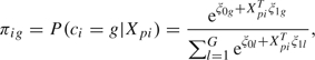
Latent class structure. Following the model formulation of Lin and others (2002) and Proust-Lima and others (2009), we assume that the population of patients after RT can be divided into G latent classes. The latent class membership is defined by a categorical latent variable c_i. The probability π_ig that subject i (i = 1,…,N) belongs to latent class g (g = 1,…,G) is related to the covariates X_pi in a multinomial logistic regression model:

(2.1)

where ${\xi }_{0g}$ is the intercept for class g and ${\xi }_{1g}$ is the vector of class-specific parameters associated with the vector of time-independent covariates $X_{pi}$. For identifiability, ${\xi }_{01}=0$ and ${\xi }_{11}=0$. In the JLCM, the latent class structure is assumed to capture the entire dependency between the biomarker trajectory and the risk of the event so that, as shown also in the directed graph in Figure S1 of supplementary material available at Biostatistics online (http://biostatistics.oxfordjournals.org), PSA trajectory and risk of recurrence are independent given the latent class membership.

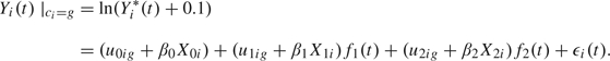
Pattern of PSA changes. Let Y_i*(t) be the value of PSA at time t for subject i, i = 1,…,N, whose times of measurements are $t_{ij},j=1,\dots ,n_i$. The PSA trajectory is described by a linear mixed model (Laird and Ware, 1982) specific to class g on the logarithm scale:

(2.2)

The parametric functions f₁ and f₂ were chosen in a preliminary analysis of 5 large cohorts of patients that described the progression of PSA after RT (Proust-Lima and others, 2008). The function f₁ represents the initial decline of PSA after the end of RT. Using a profile maximum likelihood technique for the transformation family defined by $f_1(t,\eta )=\left(\right(1+t{)}^{\eta }-1)$, we found that $\eta =-1.5$ provided the best fit. The function f₂ represents the long-term rise in PSA after the end of radiation. By considering the profile likelihood for the family of functions $f_2(t,\nu )=t^{\nu +1}/\left(\right(t+1{)}^{\nu })$, we found that $f_2(t,0)=t$ gave the best fit over the cohorts of patients. We note that this corresponds to a long-term exponential rise in PSA, which has been previously used (Pauler and Finkelstein, 2002), (Yu and others, 2004). The vector of class-specific random effects $u_{ig}=(u_{0ig},u_{1ig},u_{2ig}{)}^T$ follows a multivariate Gaussian distribution with mean vector ${\mu }_g=({\mu }_{0g},{\mu }_{1g},{\mu }_{2g}{)}^T$ and unstructured variance–covariance matrix ω_g²B, where ω₁ = 1 for identifiability. The vector μg represents the mean trajectory of ln($\text{PSA}+0.1$) over time in latent class g. The vectors $X_{0i}$, $X_{1i}$ and $X_{2i}$ are subvectors of X_i, the total vector of covariates, and are associated with PSA trajectory through the regression parameters β₀, β₁, and β₂. For the application, we chose those effects to be common over the classes. Finally, ${ϵ}_i\left(t\right)$ are independent Gaussian measurement errors with mean 0 and variance σ₂.

Risk of recurrence. Let T_i* be the time to recurrence and C_i the censoring time. The observed event time is $T_i=\text{min}(T_i^{*},C_i)$. The indicator of recurrence E_i equals 1 if $T_i^{*}\le C_i$ and 0 if $C_i\hspace{0.17em}<\hspace{0.17em}{T}_i^{*}$. We describe the risk of the event in latent class g by a proportional hazard model:

(2.3)

where $X_{ri}\left(t\right)$ is a vector of covariates that can be time dependent. We assumed that the effect of covariates on the risk of recurrence was common over the latent classes, but class-specific effects could also be specified. Finally, ${\lambda }_{0g}(t;{\zeta }_g)$ is the baseline hazard in latent class g; in our application, we used either a Weibull or a piecewise-constant risk function. The latent class structure captures all the dependency between the biomarker evolution and the time to recurrence through ${\lambda }_{0g}(t;{\zeta }_g)$, so that neither the current value of the biomarker nor any other function of the random effects appears in the survival model.

2.2. Maximum likelihood estimates

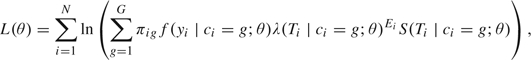
We denote by θ the vector of all the parameters. The log-likelihood of the observed data is

(2.4)

where ${\pi }_{ig}=P(c_i=g;\theta )$ is defined in (2.1) and $S(T_i\mid c_i=g;\theta )$ is the survival function derived from (2.3). The density $f(y_i\mid c_i=g;\theta )$ of the vector of PSA measures y_i in latent class g is the multivariate normal density ${\phi }_g({\tilde{y}}_i;\theta )$ with mean and variance–covariance matrix described in Proust-Lima and others (2009). For a given number of latent classes, maximum likelihood estimates are computed from (2.4) using a modified Marquardt (1963) algorithm. Convergence is assessed by stringent criteria based on the second derivatives of the log-likelihood and by using a grid of initial values. The optimal number of latent classes is determined using the Bayes information criterion (BIC) (Schwarz, 1978), as is typical in mixture models (Hawkins and others, 2001). An estimate of the variance–covariance matrix $\widehat{V}\left(\theta \right)$ of the parameters θ is given by the inverse of the Hessian matrix at the point estimate.

2.3. Posterior probability of recurrence

A posterior probability of recurrence can be easily derived from the JLCM and its parameters θ. This probability, which can be computed for a new subject using his available data at the current time, constitutes a dynamic prognostic tool of recurrence.

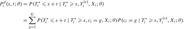
Dynamic prognostic tool derived from the joint model. Consider a new subject i free of recurrence at time s for whom the vector of repeated measures until s is denoted by $Y_i^{\left(s\right)}=\{Y_i\left(u\right),u\le s\}$ and all the covariates X_i included in (2.1–2.3) are available. Let T_i* denote the time of recurrence for subject i. Then, the posterior probability of recurrence between s and s + t for the parameter value θ can be easily computed:

(2.5)

The latent class structure entirely captures the dependence between the trajectory of the marker and the risk of recurrence. The predicted probability in (2.5) is the sum over the classes of the product of the class-specific conditional probability of the event that does not involve the marker measurements Y_i(s),

(2.6)

and the posterior probability of class membership given by

(2.7)

Posterior probability of recurrence in simpler models. The standard proportional hazard model can be viewed as a specific case of the JLCM. If G = 1, the risk of recurrence is independent of the evolution of the biomarker, and the posterior probability of recurrence given in (2.5) reduces to

(2.8)

where X_i are baseline covariates and θ the vector of parameters from the proportional hazard model given in (2.3) with G = 1.

When interest is in the prediction of an event after a certain time s, given the history of the event and covariates until that time, a model for the residual time distribution is required. A landmark (or partly conditional) model that does not specify the longitudinal process can be used (Shi and others, 1996), (Zheng and Heagerty, 2005), (Van Houwelingen, 2007), (Schoop and others, 2008). This approach consists of fitting a survival model only to subjects still at risk at time s with covariates collected until s, specifically the repeated measures of the marker. It is common to reduce this general model and use only the value of the marker at time s. In our case, this reduces to a proportional hazard model fitted on subjects free of recurrence at time s with covariates X_i and Y_i(s). A different vector of parameters θ_s is obtained for each time s, and the predictive probability of recurrence is

(2.9)

In practice, PSA is measured at discrete times, so that Y_i(s) is not observed for all s. We considered 2 landmark models that differed in the imputation of Y_i(s). First, we considered a “naive” landmark model that includes the last measure of PSA before s to approximate the value at time s. Although Prentice (1982) showed that using the last measure of the marker to approximate the current marker value could induce bias, we used that approach because we wanted to provide a very simple model that included information about PSA. Second, we instead extrapolated the value of the marker at the landmark point s using a 2-stage approach (Tsiatis and others, 1995). This method first estimates the mixed model for PSA evolution described in (2.2) with G = 1 on a training sample and then uses the estimates to compute the empirical Bayes estimates of the random effects and to estimate the PSA level at time s for any new subject based on his PSA repeated measures before s.

We note that the landmark analysis does require a separate estimation of θ_s for any time s needed for prognosis. A more complex approach proposed by Van Houwelingen (2007) defines θ_s as a parametric function of s so that θ_s can be obtained at any s.

Estimate and measure of variability. For each of the prognostic tools given by (2.5), (2.8), or (2.9), the predictive probability of recurrence for patient i before time s + t given that he was free of recurrence before time s can be computed using the vector of parameters $\widehat{\theta }$ previously estimated on a sample, as $P_i(s,t)=P_i(s,t;\widehat{\theta })$. Equivalently, the predictive probability of being free of recurrence is denoted by $S_i(s,t)=1-P_i(s,t;\widehat{\theta })$. These are point estimates. To give a measure of their variability, we approximated the Bayesian posterior distribution of $P_i(s,t)$. Vectors $({\theta }^d{)}_{d=1,\dots ,D}$ were drawn from the normal approximation of the asymptotic distribution of θ, $𝒩(\widehat{\theta },\widehat{V}(\widehat{\theta }\left)\right)$, so that the standard error could be estimated from the empirical standard deviation, . This method does not involve any further estimation procedure. It requires only the point estimate $\widehat{\theta }$ and the variance $\widehat{V}(\widehat{\theta })$ computed once from the training sample. It avoids the need for a computationally intensive bootstrap resampling scheme, and it is not model specific in comparison to the Δ-method. However, it can only be used for parametric models. The 95% confidence bands of $P_i(s,t)$ can also be obtained as the 2.5 and 97.5 percentiles of $P_i(s,t;{\theta }^d)$. The method can be extended to calculate standard errors of summary measures of predictive accuracy presented in Section 3 on testing samples. In that case, the calculation also involves bootstrapping the testing data.

3. VALIDATION OF PREDICTIVE TOOLS USING PREDICTIVE ACCURACY MEASURES

When validating and comparing predictive rules in a survival context, there is no agreement in the literature about which measures should be preferred (Pencina and others, 2008). One can be interested either in the discriminative power of the predictive rule and use concordance measures derived from receiver operating characteristic methodology (Heagerty and Zheng, 2005), (Zheng and Heagerty, 2007) or in the predictive accuracy of the rule (Schemper and Henderson, 2000). In this work, we chose to focus on predictive accuracy measures that compare the actual value of predictions with the observed data. We used summary measures derived from the error of prediction (EP), ${\text{err}}_{L;X}\left(t\right)=E\left[L\right(\eta \left(t\right)-\widehat{S}\left(t\right|X\left)\right)]$, where $\widehat{S}\left(t\right|X)$ is the predictive rule regarded as fixed, $\eta \left(t\right)$ the event status at time t, L is a loss function, and the expectation is with respect to the joint distribution of T and X. Several estimators of error of prediction were proposed either for time-independent rules (Schemper and Henderson, 2000), (Graf and others, 1999) or for dynamic rules (Henderson and others, 2002), (Schoop and others, 2008). They differ in the loss function and the method used to account for censoring. In this work, we chose to focus on the estimate of absolute EP proposed by Henderson and others (2002) that we found had the best properties in a simulation study.

For a dynamic rule $\widehat{S}(s+t|X_i\left(s\right))$, the estimator of absolute EP is computed at time s + t given information collected at time s and earlier:

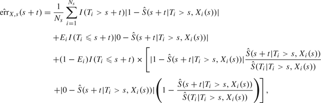(3.1)

where N_s is the number of subjects still at risk at time s.

In the dynamic prognosis context, the EP is a 2D curve so that summary measures are useful. We used 2 summary measures over a $[0,\tau ]$ window for a given time s: the absolute EP at horizon τ$\left(\text{EP}\right(\tau \left)\right)$ and the weighted average absolute error of prediction (WAEP) over $[0,\tau ]$, as proposed by Henderson and others (2002). This weighted average integrates the absolute EP over $[0,\tau ]$ using weights that correct for the reduction in the number of observed events at longer times due to censoring. The estimator of WAEP is

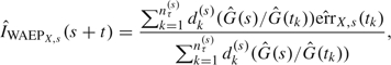(3.2)

where $d_k^{\left(s\right)}$ is the number of events at time t_k among subjects still at risk at time s and $\widehat{G}(t_k)$ and $\widehat{G}\left(s\right)$ are the Kaplan–Meier estimates of the censoring distribution at times $t_k$ and s.

Whatever the predictive accuracy measure of interest (EP(τ) or WAEP over $[0,\tau ]$), a relative measure of predictive accuracy can be developed that is analogous to R² in linear regression: the proportion of predictive accuracy explained by covariates. For example, the proportion of predictive accuracy at time t added when using covariates X₁ and X₂ rather than X₁ alone would be $({\text{err}}_{L;X_1}\left(t\right)-{\text{err}}_{L;X_1,X_2}\left(t\right))/{\text{err}}_{L;X_1}\left(t\right)$.

4. APPLICATION TO PROSTATE CANCER

4.1. Three cohort studies

We considered data from 3 large prospective cohorts of patients treated by external beam RT for localized prostate cancer. The 3 cohorts were from University of Michigan (UM) (Taylor and others, 2005), William Beaumont Hospital (WBH) (Kestin and others, 1999), and Radiation Therapy Oncology Group (RTOG9406) (Roach and others, 2004). Patients were included in the analysis if they had a clinical stage T1-4 and neither positive nodes nor metastases, they had at least 1-year follow-up without clinical recurrence or SADT, and they had at least 2 repeated measures of PSA before the end of the follow-up. The end point of interest was the first clinical recurrence so that all the PSA measures collected after the end of RT and before this point were included unless a SADT was received, in which case measures after SADT were deleted. Clinical recurrence was defined as any of the following: distant metastases, nodal recurrence, any palpable or biopsy-detected local recurrence 3 years or later after radiation; any local recurrence within 3 years of RT if the most recent PSA was >2 ng/mL; and death from prostate cancer. This definition was to allow for the possibility of residual local disease up to 3 years after RT.

Three pretreatment prognostic factors were considered: Gleason score category (2–6, 7, 8–10), T-stage category (1, 2, 3–4), and the pretreatment level of PSA (iPSA) transformed to ln(iPSA + 0.1). As the risk of recurrence should be markedly reduced after SADT, a time-dependent indicator of SADT, equal to 0 before the time of SADT and 1 after, was included in the hazard model. The 3 cohorts are described in Table 1.

Table 1.

Description of the 3 cohorts BM (N = 1268), UM (N = 503), and RTOG (N = 615), categorical variable shown as number (frequency), and continuous variables as mean (standard deviation)

Variable		BM	UM	RTOG
		(N = 1268)	(N = 503)	(N = 615)
Event		190 (15.0)	85 (16.9)	42 (6.8)
T-stage	1	431 (34.0)	163 (32.4)	348 (56.6)
	2	792 (62.5)	290 (57.7)	253 (41.1)
	3, 4	45 (3.5)	50 (9.9)	14 (2.3)
Gleason	< 7	902 (71.1)	276 (54.9)	421 (68.4)
	7	252 (19.9)	188 (37.4)	156 (25.4)
	> 7	114 (9.0)	39 (7.7)	38 (6.2)
Hormonal therapy		170 (13.4)	44 (8.8)	47 (7.6)
ln(iPSA + 0.1) (ln(ng/mL))		2.16 (0.84)	2.23 (0.92)	2.00 (0.61)
Age (years)		72.7 (6.5)	69.0 (7.1)	68.0 (7.0)
Time to recurrence (years)		5.03 (2.71)	3.82 (2.49)	4.61 (2.00)
Time to last contact (years)		5.91 (3.30)	6.21 (3.41)	5.92 (2.03)

A prognostic tool should be validated on external data, that is data not used for the creation of the prognostic tool. Following the validation strategy suggested by Altman and Royston (2000), we developed the prognostic tool on WBH, the largest cohort, and evaluated its predictive performances on 2 external samples, UM and RTOG9406. Although they are different cohorts, WBH and UM were comparable in terms of pretreatment covariates (T-stage, Gleason, and iPSA) and proportion of recurrences, whereas subjects in RTOG9406 were usually in a earlier stage of the disease with a larger proportion of subjects with T-stage 1 and Gleason below 7. The number of recurrences in RTOG9406 was also smaller (6.8% versus 16.9% and 15.0% in WBH and UM).

4.2. Estimation of the JLCM on WBH

The 3 baseline covariates were included in both the survival model and the latent class membership model. For the mixed model, as recommended by Proust-Lima and others (2008), Gleason was only included in the long-term rise part of the model while T-stage was included in both short-term and long-term parts, and iPSA was included in all 3 terms in (2). The hazard was defined by a class-specific Weibull function since the Akaike criterion was systematically better compared to a 5-step hazard function. The JLCM was fitted for different numbers of classes. The values of BIC as the number of classes varied from 2 to 6 were 13 514.5, 13 386.2, 13 347.6, 13 327.1, and 13 354.5, respectively, and the associated numbers of parameters were 39, 51, 63, 75, and 87. The class-specific predicted mean trajectories and survival functions are displayed in Figure 1. The latent classes differed mainly by their long-term rise of PSA and the risk of recurrence, a higher long-term increase of PSA being associated with a higher risk of recurrence. Classes 1 and 2, which were relatively close in terms of trajectory and risk of recurrence, were different in terms of class membership parameters.

Fig. 1.

(A) Predicted mean evolution and (B) survival function in the 5 latent classes of the selected JLCM on WBH data (N = 1268). Predictions given for a subject with T-stage = 2, Gleason = 7, and iPSA = 10 n/mL.

4.3. Dynamic prediction of prostate cancer recurrence

To illustrate the use of the posterior probabilities of recurrence at time s + t given the information collected until time s, we show in Figure 2 the predicted probability of recurrence for 2 patients from the UM cohort. For each one, the predicted cumulative risk of recurrence was computed using the JLCM (denoted 5-LCM), the proportional hazard model with baseline covariates and a 5-step risk function (denoted baseline), and the 2-stage landmark model with a 5-step risk function (denoted PSA(s)). Predicted probabilities using the naive landmark model with the latest PSA measure were very similar to the 2-stage landmark model. The 95% confidence bands were computed as described in Section 2.3 using 2000 draws. Predictions were made up to 3 years ahead, which is a reasonable time horizon in this clinical setting.

Fig. 2.

Individual prediction of prostate cancer recurrence for 2 patients from UM. On the left, the patient experienced a recurrence 3.8 years after RT. Updated individual predictions are given every 6 months from 1 to 3.5 years. On the right, the patient did not experience any recurrence within the first 6 years after RT. Updated individual predictions are given every year from 1 to 6 years after RT. The x are the PSA measures used for the prediction, the vertical solid line is the time s of prediction, and the vertical dashed line is the time of recurrence.

For the subject on the left who recurred within the first 4 years, updated risk of recurrence was computed every 6 months from 1 to 3.5 years after the end of RT. The PSA pattern for this patient is characteristic of an early recurrence with a drop of PSA the first year after the end of RT and a subsequent rise of PSA. However, levels of PSA are relatively low. The 5-LCM-based prediction that accounts for the shape of the PSA trajectory rather than the level of PSA captures the high risk of recurrence, while the PSA(s) level–based prediction remains relatively low. In supplementary material available at Biostatistics online, Figures S2 and S3 show predictions for 3 other patients (Rec2, Rec3, Rec4) with different PSA profiles who recurred. For each of them, the 5-LCM model detects higher risk of recurrence earlier after the end of RT.

For the subject on the right who did not experience any recurrence within 6 years after RT, the updated risk of recurrence was computed every year from 1 to 6 years. This subject has a PSA trajectory characteristic of a cured patient. However, as he has relatively bad prognostic factors (T-stage=3, Gleason=8, and iPSA=62.4 ng/mL), the prediction based on baseline covariates predicts a high probability of recurrence while the 2 dynamic prognostic tools update the risk of recurrence according to the PSA trajectory so that, as soon as 3 years after RT, the probabilities of recurrence they provide become very low. In supplementary material available at Biostatistics online, predictions for a second cured patient (Cens1 in Figure S4) also show how accounting for PSA repeated measures allows a better understanding of the cancer progression.

These individual predictions underline the usefulness of dynamic prognostic tools that can adapt to the PSA trajectory. In Section 4.4, we used predictive accuracy measures to corroborate these suggestions at a population level on the UM and RTOG data sets.

4.4. Validation of the prognostic tool on UM and RTOG

We evaluated the predictive accuracy of the prognostic tool based on the JLCM 4 times a year from s = 1 year to s = 6 years after the end of RT for a time horizon of 3 years. For each s, we computed the absolute EP curves and displayed 3 summary measures: the weighted average absolute error of prediction (WAEP) over 3 years and the EP at 1- and 3-year horizons. The 5-latent class model (denoted 5-LCM) performances were compared to those of a proportional hazard model including baseline covariates and a 5-step risk function (denoted baseline), a proportional hazard model with a 5-step risk function but without any covariate (denoted no covariate), and 2 landmark models with a 5-step risk function (denoted either PSA(s) or last PSA depending on how the level of PSA at time s was computed). The summary measures for cohort UM and RTOG are displayed in Figure 3. The estimates and standard errors of WAEP in the 5-LCM model for UM and RTOG cohorts were 0.0816 (SE=0.0090) and 0.0422 (SE=0.0068), respectively, after 1-year follow-up and 0.0614 (SE=0.0095) and 0.0472 (SE = 0.0074), respectively, after 3-year follow-up. Table 2 gives the relative gain in WAEP for the 2 landmark models and the JLCM compared to the model including only baseline information.

Fig. 3.

Weighted average absolute error of prediction (WAEP) over 3 years of forecast and EP at a forecast of, respectively, 1 year and 3 years using the absolute loss function for UM cohort (on the left) and RTOG cohort (on the right).

Table 2.

Relative gain (in %) of WAEP over 3 years of forecast for the 2 landmark models (last PSA and PSA(s)) and the 5-class JLCM compared to the proportional hazard model with baseline information. Gain in WAEP are computed from s = 1 to s = 6 years after RT and are given for each cohort UM and RTOG

Cohort	Time	Landmark models		JLCM
	s	Last PSA	PSA(s)
UM	1	3.2	3.3	11.7
	2	7.7	7.7	15.3
	3	17.6	19.5	13.7
	4	7.2	11.3	8.9
	5	5.9	9.5	8.4
	6	19.9	19.5	7.3
RTOG	1	4.8	4.2	18.4
	2	9.2	9.0	24.9
	3	19.2	25.1	26.7
	4	17.4	20.0	24.7
	5	12.6	8.9	14.8
	6	3.1	1.5	12.8

For UM, whatever the summary measure, inclusion of baseline covariates improved the predictive accuracy for prostate cancer recurrence only when using information from the first 3 years (s ≤ 3). After that point, the model without covariates gave similar predictive accuracy even though covariates effects were highly significant. Accounting for the PSA measures in addition to the baseline covariates using either a joint model or a landmark model reduced markedly the absolute EP in the first 6 years with relative gain in WAEP varying from 3% to close to 20% (see Table 2). Moreover, the joint model improved the predictive accuracy more than the landmark models when using information from 1 year (11.7% versus 3.3% of gain compared to baseline information) to 2 years (15.3% versus 7.7% of gain) after RT while the landmark models gave a better predictive accuracy at s = 6 (gain of > 19.5% versus 7.3% for JLCM). This means that in the first 2 years, the expected PSA at time of landmark was not sufficiently predictive, while later the level of PSA mainly drove the predictions for UM.

For the RTOG cohort, the baseline covariates improved the predictive accuracy during the whole follow-up. Furthermore, accounting for PSA repeated measures improved markedly the predictive accuracy by reducing the absolute error during the whole follow-up and especially in the first 2 years, as seen also in Table 2 with gain in WAEP of 18.4% or 24.9% at 1 and 2 years versus <4.8% and <9.2% for the landmark models. In this cohort, which included earlier stages of the disease, the landmark models did not capture all the predictive value of the PSA trajectory, underlining the relevance of models like JLCM that include the whole trajectory. For the 2 cohorts, the 2 landmark models gave similar predictiveness.

From a specific time of prediction, the curve of EP describes the change in EP over horizon of prediction (Figure 4). At 1 year after RT, including the posttreatment PSA measures in the JLCM substantially reduced the EP for the UM cohort at any horizon compared to the proportional hazard model including baseline covariates (e.g. 19% improvement at 3-year horizon while including the expected PSA(s) value improved the predictive accuracy by only 5% at 3-year horizon). In contrast, when using information until 3 years after RT, the landmarking analysis EP approached or surpassed the joint model EP suggesting that after a time, the level of PSA may be sufficient for determining the risk of recurrence for UM. Conversely, for RTOG cohort, both from 1 year and 3 years after RT, the joint model reduced markedly the EP at any horizon compared to the landmarking analysis.

Fig. 4.

Absolute EP for UM cohort (on the left) and RTOG cohort (on the right) based on information at s = 1,2,3 and for a forecast up to 3 years in the future.4

5. DISCUSSION

Although it is well known that PSA is highly predictive of prostate cancer recurrence, its use for monitoring progression of the disease is still rather limited and typically restricted to a binary summary of the PSA dynamics. Joint models offer an efficient framework to quantify the probability of recurrence utilizing the repeated measures of PSA. We have shown how a JLCM could be used to provide a dynamic prognostic tool of recurrence that can be updated for each new measurement of PSA. The methodology would be similar for a shared random-effects model, except that the computations would be more burdensome (Pauler and Finkelstein, 2002), (Yu and others, 2004). The JLCM relies on the conditional independence of the PSA repeated measures and the recurrence of prostate cancer given the latent classes. The practical advantages of this are that the log-likelihood has a closed form and that the predictive tool can be computed analytically. The construction of the tool requires the estimation of the parameters on a single population only once. The prognostic tool can then be computed analytically for any new subject, using any information about PSA repeated measures and at any time. Moreover, to aid the user in evaluating the variability of the prediction, standard error and confidence bands are computed using an approximation of the Bayesian posterior distribution. This technique can be used for parametric rules whenever the Δ-method is not straightforward and a bootstrap is too computationally intensive. One limitation of the JLCM would be that the number of latent classes cannot be directly estimated and has to be selected according to a criterion, commonly the BIC. We note that using BIC to choose the number of classes has become standard practice in mixture modeling (e.g. (Hawkins and others, 2001)). Furthermore, we found that the predictive accuracy was not markedly impacted by the choice of the number of latent classes. For example, the gain in predictive accuracy compared to the PHM with baseline covariates was roughly the same for 4–6 latent classes (e.g. gain in WAEP for RTOG: 16.5%, 17.5%, 22.5%, 21.6%, and 19.8% for G=2, 3, 4, 5, and 6).

The validation of prognostic tools on different cohorts is of primary importance in the process of developing a prognostic tool, especially when using a complex statistical model. Indeed, a complex model can be fine tuned for the data set on which it is estimated but have a poor fit on new data. Following the Altman and Royston (2000) hierarchy of increasingly stringent validation strategies, we directly validated our model on different data sets, from other centers and other investigators. That gave us a good appreciation of whether a prognostic tool based on a relatively complex model may improve the predictive accuracy in practice. We found that the landmark approaches gave similar predictive accuracy as a joint model for one data set, but its predictive accuracy was lower for the other data set, suggesting its potential lack of generalizability. For these 2 data sets, we found consistently that updating the risk of recurrence using the trajectory of PSA was an important refinement and that, at least in the first years, the level of PSA at time of prognosis could not capture the whole predictiveness of the PSA trajectory.

There are many choices for how to validate a model (Pencina and others, 2008). We chose predictive accuracy measures that focus on predictiveness rather than discrimination. Measures of predictive accuracy have been criticized because of their lack of interpretation. We showed through the application that our chosen measures give an easily interpretable assessment of the relative gain by quantifying the gain in predictiveness of a new model compared to a standard one.

To conclude, joint modeling of a marker trajectory and a clinical outcome is an attractive approach for developing powerful prognostic tools that can help clinical decision making in chronic diseases. Predictive accuracy measures offer an umbrella of criteria on which a prognostic tool can be validated and compared to other existing rules.

FUNDING

US National Cancer Institute (CA110518; CA21661); post-doctoral fellows from Les Entreprises du Médicament recherche France.

SUPPLEMENTARY MATERIAL

Supplementary Material is available at http://www.biostatistics.oxfordjournals.org.

References

- Altman DG, Royston P. What do we mean by validating a prognostic model? Statistics in Medicine. 2000;19:453–473. doi: 10.1002/(sici)1097-0258(20000229)19:4<453::aid-sim350>3.0.co;2-5. [DOI] [PubMed] [Google Scholar]
- D'Amico AV, Moul J, Carroll PR, Sun L, Lubeck D, Chen MH. Prostate specific antigen doubling time as a surrogate end point for prostate cancer specific mortality following radical prostatectomy or radiation therapy. Journal of Urology. 2004;172:S42–S46. doi: 10.1097/01.ju.0000141845.99899.12. [DOI] [PubMed] [Google Scholar]
- Graf E, Schmoor C, Sauerbrei W, Schumacher M. Assessment and comparison of prognostic classification schemes for survival data. Statistics in Medicine. 1999;18:2529–2545. doi: 10.1002/(sici)1097-0258(19990915/30)18:17/18<2529::aid-sim274>3.0.co;2-5. [DOI] [PubMed] [Google Scholar]
- Hawkins DS, Allen DM, Stromberg AJ. Determining the number of components in mixtures of linear models. Computational Statistics and Data Analysis. 2001;38:15–48. [Google Scholar]
- Heagerty PJ, Zheng Y. Survival model predictive accuracy and ROC curves. Biometrics. 2005;61:92–105. doi: 10.1111/j.0006-341X.2005.030814.x. [DOI] [PubMed] [Google Scholar]
- Henderson R, Diggle P, Dobson A. Joint modelling of longitudinal measurements and event time data. Biostatistics. 2000;1:465–480. doi: 10.1093/biostatistics/1.4.465. [DOI] [PubMed] [Google Scholar]
- Henderson R, Diggle P, Dobson A. Identification and efficacy of longitudinal markers for survival. Biostatistics. 2002;3:33–50. doi: 10.1093/biostatistics/3.1.33. [DOI] [PubMed] [Google Scholar]
- Kestin LL, Vicini FA, Ziaja EL, Stromberg JS, Frazier RC, Martinez AA. Defining biochemical cure for prostate carcinoma patients treated with external beam radiation therapy. Cancer. 1999;86:1557–1566. doi: 10.1002/(sici)1097-0142(19991015)86:8<1557::aid-cncr24>3.0.co;2-2. [DOI] [PubMed] [Google Scholar]
- Laird NM, Ware JH. Random-effects models for longitudinal data. Biometrics. 1982;38:963–974. [PubMed] [Google Scholar]
- Lin H, Turnbull BW, McCulloch CE, Slate EH. Latent class models for joint analysis of longitudinal biomarker and event process data: application to longitudinal prostate-specific antigen readings and prostate cancer. Journal of the American Statistical Association. 2002;97:53–65. [Google Scholar]
- Marquardt D. An algorithm for least-squares estimation of nonlinear parameters. SIAM Journal on Applied Mathematics. 1963;11:431–441. [Google Scholar]
- Pauler DK, Finkelstein DM. Predicting time to prostate cancer recurrence based on joint models for non-linear longitudinal biomarkers and event time outcomes. Statistics in Medicine. 2002;21:3897–3911. doi: 10.1002/sim.1392. [DOI] [PubMed] [Google Scholar]
- Pencina MJ, D'Agostino RB, Sr, D'Agostino RB, Jr, Vasan RS. Evaluating the added predictive ability of a new marker: from area under the ROC curve to reclassification and beyond. Statistics in Medicine. 2008;27:157–172. doi: 10.1002/sim.2929. [DOI] [PubMed] [Google Scholar]
- Prentice RL. Covariate measurement errors and parameter estimation in Cox's failure time regression model. Biometrika. 1982;69:331–342. [Google Scholar]
- Proust-Lima C, Joly P, Dartigues J-F, Jacqmin-Gadda H. Joint modelling of multivariate longitudinal outcomes and a time-to-event: a nonlinear latent class approach. Computational Statistics and Data Analysis. 2009;53:1142–1154. [Google Scholar]
- Proust-Lima C, Taylor JMG, Williams SG, Ankerst DP, Liu N, Kestin LL, Bae K, Sandler HM. Determinants of change of prostate-specific antigen over time and its association with recurrence following external beam radiation therapy of prostate cancer in 5 large cohorts. International Journal of Radiation Oncology, Biology, Physics. 2008;72:782–791. doi: 10.1016/j.ijrobp.2008.01.056. [DOI] [PMC free article] [PubMed] [Google Scholar]
- Roach M, Hanks G, Thames H, Schellhammer P, Shipley WU, Sokol GH, Sandler HM. Defining biochemical failure following radiotherapy with or without hormonal therapy in men with clinically localized prostate cancer: recommendations of the RTOG-ASTRO Phoenix Consensus Conference. International Journal of Radiation Oncology, Biology, Physics. 2006;65:965–974. doi: 10.1016/j.ijrobp.2006.04.029. [DOI] [PubMed] [Google Scholar]
- Roach M, Winter K, Michalski JM, Cox JD, Purdy JA, Bosch W, Lin X, Shipley WS. Penile bulb dose and impotence after three-dimensional conformal radiotherapy for prostate cancer on RTOG 9406: findings from a prospective, multiinstitutional, phase i/ii dose-escalation study. International Journal of Radiation Oncology, Biology, Physics. 2004;60:1351–1356. doi: 10.1016/j.ijrobp.2004.05.026. [DOI] [PubMed] [Google Scholar]
- Sartor CI, Strawderman MH, Lin XH, Kish KE, McLaughlin PW, Sandler HM. Rate of PSA rise predicts metastatic versus local recurrence after definitive radiotherapy. International Journal of Radiation Oncology, Biology, Physics. 1997;38:941–947. doi: 10.1016/s0360-3016(97)00082-5. [DOI] [PubMed] [Google Scholar]
- Schemper M, Henderson R. Predictive accuracy and explained variation in Cox regression. Biometrics. 2000;56:249–255. doi: 10.1111/j.0006-341x.2000.00249.x. [DOI] [PubMed] [Google Scholar]
- Schoop R, Graf E, Schumacher M. Quantifying the predictive performance of prognostic models for censored survival data with time-dependent covariates. Biometrics. 2008;64:603–610. doi: 10.1111/j.1541-0420.2007.00889.x. [DOI] [PubMed] [Google Scholar]
- Schwarz G. Estimating the dimension of a model. Annals of Statistics. 1978;6:461–464. [Google Scholar]
- Shi M, Currier RJ, Taylor JMG, Tang H, Hoover DR, Chmiel JS, Bryant J. Replacing time since HIV infection by marker values in predicting residual time to AIDS diagnosis. Journal of Acquired Immune Deficiency Syndromes. 1996;12:309–316. doi: 10.1097/00042560-199607000-00013. [DOI] [PubMed] [Google Scholar]
- Taylor JMG, Yu M, Sandler HM. Individualized predictions of disease progression following radiation therapy for prostate cancer. Journal of Clinical Oncology. 2005;23:816–825. doi: 10.1200/JCO.2005.12.156. [DOI] [PubMed] [Google Scholar]
- Thompson IM, Ankerst DP, Chi C, Lucia MS, Goodman PJ, Crowley JJ, Parnes HL, Coltman CA., Jr Operating characteristics of prostate-specific antigen in men with an initial PSA level of 3.0 ng/ml or lower. Journal of the American Medical Association. 2005;294:66–70. doi: 10.1001/jama.294.1.66. [DOI] [PubMed] [Google Scholar]
- Tsiatis AA, DeGruttola V, Wulfsohn MS. Modeling the relationship of survival to longitudinal data measured with error. Applications to survival and CD4 counts in patients with AIDS. Journal of the American Statistical Association. 1995;90:27–37. [Google Scholar]
- Van Houwelingen HC. Dynamic prediction by landmarking in event history analysis. Scandinavian Journal of Statistics. 2007;34:70–85. [Google Scholar]
- Yu M, Law NJ, Taylor JMG, Sandler HM. Joint longitudinal-survival-cure models and their application to prostate cancer. Statistica Sinica. 2004;14:835–862. [Google Scholar]
- Zheng Y, Heagerty PJ. Partly conditional survival models for longitudinal data. Biometrics. 2005;61:379–391. doi: 10.1111/j.1541-0420.2005.00323.x. [DOI] [PubMed] [Google Scholar]
- Zheng Y, Heagerty PJ. Prospective accuracy for longitudinal markers. Biometrics. 2007;63:332–341. doi: 10.1111/j.1541-0420.2006.00726.x. [DOI] [PubMed] [Google Scholar]
Associated Data
This section collects any data citations, data availability statements, or supplementary materials included in this article.